
Equation 4.1 Capital Gains Tax Scaling Factor

In this chapter we continue down the path of returns-based expected utility optimization. We will create the joint return distribution forecast to feed into our optimizer, alongside the client utility function. Our starting point for this process is the full set of historical monthly returns for the assets we have selected. We introduce two techniques that help diagnose whether the historical return series is a reliable source for future expectations. The chapter ends with a review of how to modify our historical monthly return dataset for custom forecasts, manager selection, fees, and taxes.
Key Takeaways:
Thus far, we have fully specified our client's utility function by careful assessment of their risk preferences and financial situation. And we have chosen the assets that are worthwhile for us to include in our client's portfolio. The last thing we must do before running our optimizer is create the full set of possible outcomes as required by Eq. (1.2), where each outcome is a joint monthly return for all of our assets. We are not forecasting individual moments or co-moments, as is done in mean-variance asset allocation; rather, we are forecasting every single possible combination of monthly returns our assets could ever experience. Since this is an incredibly challenging task (given the complexity of financial markets which lead to joint return distributions of nuanced shape), we must look for a simple way to do this. Luckily, we can use the historical joint return distribution for our assets as our baseline forecast.
As discussed in Chapter 1, there are two conditions that must be met for a historical monthly return distribution to be a good forecast over long horizons. The first is that our sample size T (the number of monthly data points we have) must be large to ensure the accuracy of our estimation, as you need many data points to accurately diagnose the properties of a distribution. To this end, we introduce the concept of standard error, which we use to measure the uncertainty of the moment estimates that are embedded in the historical distributions we are deploying (we say “embedded” because we don't actually deploy the moment estimate in our model; we just analyze the moment error bars as a validation tool). Second, our return distribution must be stationary over long horizons so that we can assume the past will represent the future. To this end, we introduce the Kolmogorov–Smirnov test, which informs us whether the return distribution from one long period resembles the return distribution from a previous long period, indicating a stable return process where history can be trusted as a forecast.
We will also need to be able to modify the forecasts encapsulated by the historical distribution. There are many reasons why one would want to modify the historical distribution before inputting it into the optimizer. One may want to account for secular trends in risk premia. Many advisors also want to pursue active managers who can add alpha to the core asset class proposition. Fees and taxes are also critical components of real-world investments that should be accounted for. To this end, we will introduce a simple system for adjusting historical return distributions for these typical situations by shifting the entire monthly return distribution by a constant (except for capital gains taxes, which require a scaling of returns due to the government's active partnership in sharing our losses).
But before we get into the weeds, the reader might be wondering why the litany of popularized forecasting models are in a chapter on capital market assumptions (for a nice review of many of these, see Maginn, Tuttle, Pinto, & McLeavey, 2007). First, there is the question of timeframe. From the very beginning we have been focused on 10-year forecasts and beyond, precluding the use of any models with a tactical forecasting horizon (6–12 months) or opportunistic forecasting horizon (3–5 years). This removes from our purview both price-based momentum and mean reversion models, along with most fundamental models (e.g. the dividend discount model where dividend and growth forecasts typically cover the next five years). Also related to horizon, there are models (e.g. reverse optimizing the market portfolio) that incorporate information about all possible time horizons that would mis-serve us as we try to isolate just the 10-year and longer horizon.
Second, we have avoided so-called “structured” models (e.g. APT, shrinkage, etc.). In Chapter 1, we reviewed the virtues of adding structure to our estimates in the form of ML and Bayesian models to gain accuracy at the expense of introducing bias into our estimates (see Figure 1.6). For example, rather than just using historical distributions, we could have assumed a functional form for our return distributions and their interaction, to account for both heavy tails and non-linear comovement. This assumption would potentially improve our estimation error, but it would introduce additional mathematical complexity and force a specific return distribution into our assumptions. For conceptual simplicity, and to avoid approximation error associated with assuming specific distributional forms, we have avoided imposing structure into our estimation process. There are also equilibrium models (e.g. CAPM, reverse optimization of the global market portfolio, etc.) but these have their own issues. For example, reverse optimizing a market portfolio requires a number of assumptions whose validity we cannot necessarily confirm, such as how different investors model markets, how liquidity needs affect their allocations, how taxes affect their allocations, and so on. Hence, these models introduce other estimation errors we steer clear of in favor of more transparent estimation headwinds.
Our goal is a modern yet practical asset allocation process, and hopefully by the end of this chapter you will be left with a forecasting toolkit that fulfills both goals. Before we dive in, let me preface everything we are about to do with the simple disclaimer that all estimation has error bars, and the entire intent here is to provide something with strong foundational underpinnings and transparent error bars, not a holy grail with perfect accuracy.
We have two requirements for the historical monthly return distribution to be a useful long-horizon forecast: (1) we have enough data to be able to make an accurate assessment of the assets we are investing in; and (2) our assets must be stationary over long periods. Let's first refine our understanding of these requirements with a quick detour on “stochastic processes.” This explanation will help the reader build confidence in the systematic process we are building here.
The basic assumption behind using the historical joint return distribution of financial assets as a forecast is that the monthly returns are created by a well-defined stochastic process that repeats, and as long as we can measure it enough times we can get a solid grasp of the process's character. Let's carefully dissect this sentence.
A stochastic process is something that creates the random outcomes observed. In this case, the process is human beings investing in financial markets, and the outcomes are the joint monthly returns of said financial assets. Every day humans buy and sell these assets, and if their behavior and the world they live in don't change too much, then the process that defines monthly returns should be stable in time. So, unless something dramatic happens in our world, such as wild inflation or major tax code changes, the appeal and motivation of buying and selling financial assets will stay constant and the stochastic process can be treated as “stationary,” or stable in time.
What exactly does stable mean in this context? It simply means that the precise form of the joint return distribution is the same from one era (of a few decades) to the next. We all know return distributions over short and even intermediate term horizons can be very different, but we are focused on horizons greater than 10 years; hence, momentum and mean reversion effects should not get in our way when it comes to stationarity.
Assuming our underlying process is stable, we can conclude that the historical distribution we have observed is just a sample of the process's true distribution, meaning that our historical data points are just a random selection of the possible outcomes that the process can ultimately generate. From Stats 101, we know that when we use a sample to represent a true distribution, there are error bars on our estimates, formally known as the “standard error” by statisticians. This error gets smaller as we increase the sample size, eventually approaching zero as our sample size goes to infinity, giving us a perfect portrayal of the process through its observed outcomes.
In our returns-based optimization framework we are not estimating moments, though. Rather, we are using the entire distribution as the input to our optimizer. So, what exactly would we measure error bars on? Even though we deploy the full return distribution as our forecast, we still have implied estimates of all the distribution's moments that are being utilized by the optimizer. Recall from Chapter 1 that we can fully specify any distribution by an infinite set of moments. Hence, we can analyze the standard errors of the implied moments to assess whether we have enough data for our historical distribution to be a good estimate of the true distribution to present to the optimizer.1
With our refined understanding of stochastic processes, and how simple assumptions like stationarity and large sample size can assist us in forecasting, let's now turn to our first key requirement: large sample sizes.
How do we measure the standard error? Many of you have probably seen an analytic formula for the standard error of a mean estimated from a distribution of ![]() where
where ![]() is the volatility of the sample and T is the number of data points. Analytic estimates of this type are available for higher moments as well, but the derivation of these formulas generally requires making assumptions about the type of distribution the data comes from (Wright & Herrington, 2011). For example, the standard error of the mean just reviewed assumes a normal underlying distribution. Given our penchant to avoid parametric estimation methods, where we have to define the functional form of the distribution, we will be avoiding analytic formulas for standard errors.
is the volatility of the sample and T is the number of data points. Analytic estimates of this type are available for higher moments as well, but the derivation of these formulas generally requires making assumptions about the type of distribution the data comes from (Wright & Herrington, 2011). For example, the standard error of the mean just reviewed assumes a normal underlying distribution. Given our penchant to avoid parametric estimation methods, where we have to define the functional form of the distribution, we will be avoiding analytic formulas for standard errors.
Instead, we will deploy a bootstrap, one of the most beautiful statistical tools out there, which will be invaluable not just here, but also in Chapter 5 when we study the accuracy of our optimizer-recommended portfolios. Rather than use the entire sample to estimate a moment, a bootstrap uses a random sample of the full dataset to estimate the moment and then repeats that process multiple times to create a distribution of the estimate itself. The standard deviation of that distribution is then the standard error for the estimate. So, we create a number of estimates by randomly sampling our data to see how much those estimates vary—an intuitive means of assessing the accuracy of our estimate. Let's go through an example to flesh out all the details of deploying a bootstrap for calculating standard errors.
Say we have monthly returns for US equities from 1972–2018, giving us 564 data points.2 Instead of just creating a mean estimate from those 564 data points, we want to create 1,000 different estimates, where each estimate also utilizes 564 data points; but those data points are randomly sampled. They are not the same as the original set of data points, since we create a new set with replacement—which means if a return is drawn from the original data set, it may be drawn again within the same estimate.
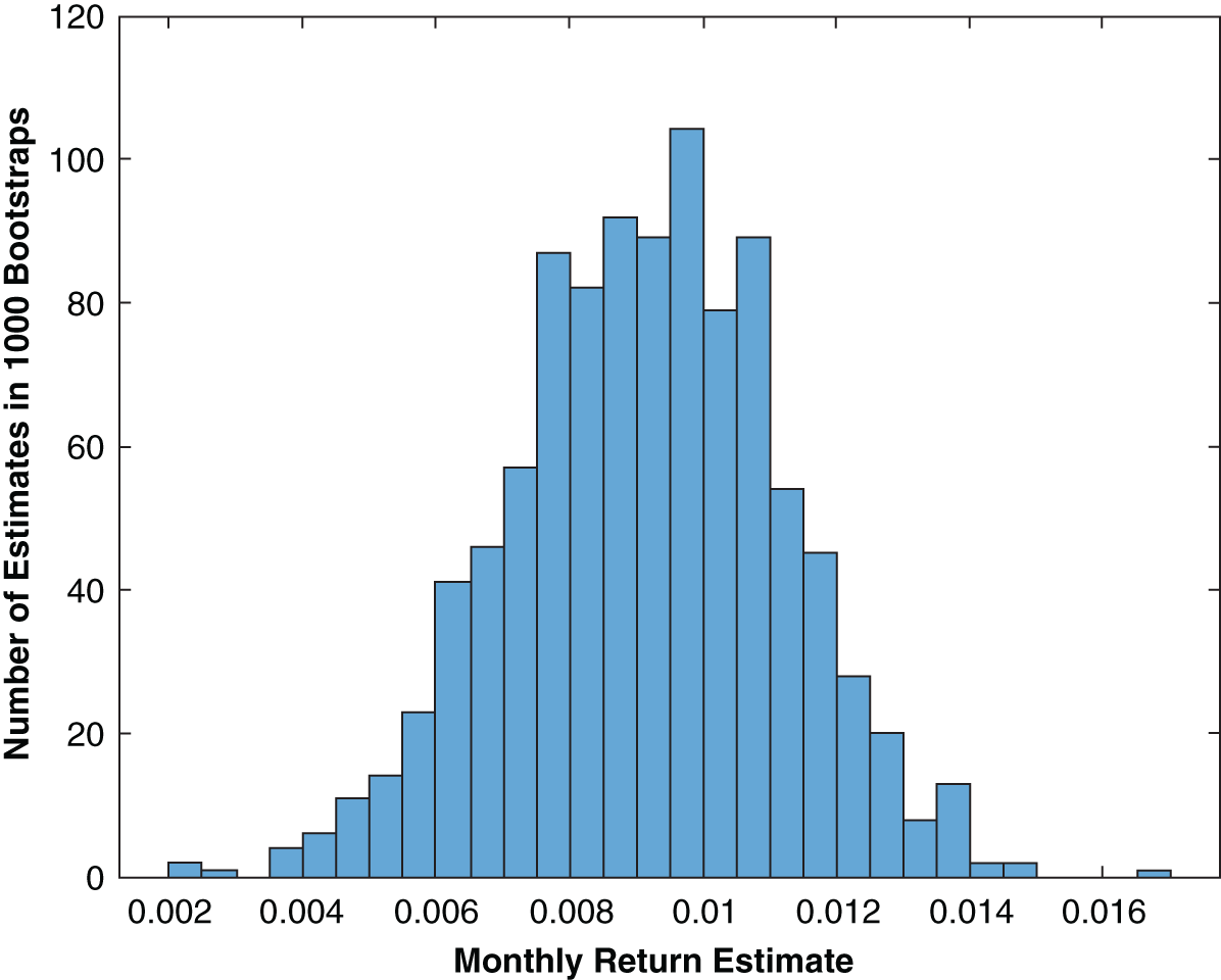
FIGURE 4.1 Bootstrap Estimates of Average Monthly Return for US Equities
Figure 4.1 shows the distribution of mean estimates from just such a procedure. The mean monthly return estimate from the original 564 data points is 0.0092, which is roughly the center of the distribution in Figure 4.1; however, now we have a distribution of estimates with a clear width. The standard error is then the standard deviation of the bootstrap distribution (it is 0.0018 for the specific 1,000 data sets used in this simulation, but because it is random it changes each time we run the bootstrap).
It is instructive now to follow standard practice and convert this standard error to error bars by multiplying the standard error by two and having our error bars be symmetric around the point estimate. Hence, our estimate of the mean monthly return for US equities based on the historical return distribution is ![]() . If we assume that the bootstrapped estimate distribution is normally distributed,3 we can deploy standard statistical significance tests that imply we can be 95% confident that the moment we are estimating lies within the error bar range around our estimate.
. If we assume that the bootstrapped estimate distribution is normally distributed,3 we can deploy standard statistical significance tests that imply we can be 95% confident that the moment we are estimating lies within the error bar range around our estimate.

FIGURE 4.2 Standard Error of First Four Moment Estimates for US Equities as a Function of Sample Size
Figure 4.2 extends this analysis for US equities to the first four moments, and plots the standard error for each moment as a function of sample size, where we vary the sample size of the data being studied backward from the last data point. For example, a sample size of 12 uses data from March 2018 to February 2019, a sample size of 24 uses data from March 2017 to February 2019, and so on. The mean and volatility standard errors are plotted on the left axis while the skew and kurtosis standard errors are plotted on the right axis. Staying focused on the mean standard error for the moment, you can see the standard error drops precipitously as sample size is increased, confirming our assertion that large sample size is paramount for good estimation. And, of course, as our sample size approaches the original 564 used earlier, we see the mean standard error approach our previous result of 0.18%.
Another key observation from Figure 4.2 is that the standard error improvement, once you go beyond 400 samples or so, becomes marginal, a result that is consistent across moments. This leads us to a critical conclusion: using historical data for forecasting should minimally include around 30 years of data but going beyond 50 or so is not overwhelmingly valuable, since standard errors barely improve for each decade added, and we simultaneously include potentially irrelevant data from periods of time unlike that of the current markets.4 Also apparent in Figure 4.2 is that our higher moment standard errors seem to take a bit longer to reach a steady state value. Hence, for improved higher moment accuracy we should really be pushing our sample size to 40–50 years, instead of just 30 years.
In case you haven't noticed, let me say that we are in a bit of a pickle. Our US equity mean estimate ![]() has sizable error bars that we cannot improve upon by extending our data further back, because we would start to utilize data that was most certainly driven by a different process than it is today (and data isn't even available for most financial assets more than a few decades back). I would assert, though, that while our mean estimate for US equities has sizable error bars, it still paints a clear picture that an equity risk premium exists5 and should be something we pursue for our clients, especially given the simple fact that we have many credible a priori theoretical reasons for these moments to be significant. Hence, we can have greater conviction that we are simply in a tight spot because of data limitations. In the world of noisy estimation of economically and behaviorally motivated processes with limited data, we are actually doing fine with these error bars.6 And for all those dogmatic practitioners out there who say historical estimates are useless unless you have hundreds of years of data (indeed, needed, if you want, say, ±1% error bars on annualized equity return forecasts), please step up and show me a model you have with better error bars.7 And yes, this same logic applies to our noisy estimates of skew and kurtosis as well.
has sizable error bars that we cannot improve upon by extending our data further back, because we would start to utilize data that was most certainly driven by a different process than it is today (and data isn't even available for most financial assets more than a few decades back). I would assert, though, that while our mean estimate for US equities has sizable error bars, it still paints a clear picture that an equity risk premium exists5 and should be something we pursue for our clients, especially given the simple fact that we have many credible a priori theoretical reasons for these moments to be significant. Hence, we can have greater conviction that we are simply in a tight spot because of data limitations. In the world of noisy estimation of economically and behaviorally motivated processes with limited data, we are actually doing fine with these error bars.6 And for all those dogmatic practitioners out there who say historical estimates are useless unless you have hundreds of years of data (indeed, needed, if you want, say, ±1% error bars on annualized equity return forecasts), please step up and show me a model you have with better error bars.7 And yes, this same logic applies to our noisy estimates of skew and kurtosis as well.
Don't forget that our approach to handle estimation error was not just to minimize estimation error but also to carefully minimize our framework's sensitivity to estimation error. Hence, shrinking our error bars is not the only tool we have to combat estimation error. Chapter 3 had us very focused on only investing in assets that were very distinct. Motivated by the fact that our forecasting error bars are indeed larger than we would like, we need to be sure we are not investing in assets that are similar enough to require very precise estimates (recall Figure 1.5, where 1% error bars lead to wildly different asset allocations). Ultimately, the key lesson here is to always try to deploy around 50 years of historical data as the starting point for your joint distribution forecasts, and minimize the number of closely related assets in your portfolio to minimize the effects of the large error bars contained within the forecast distribution.
Is there any way for us to get more comfortable with the error bars we are sitting with? Potentially. It is well known that the estimation of a distribution via historical data is sensitive to outliers. Figure 4.3 plots the same bootstrap exercise we just went through to find standard errors for our first four moments, but with one key difference: we have removed the most extreme positive and negative monthly returns from the dataset (a total of two data points out of 564). As you can see, the standard errors shrink by “winsorizing” just the top and bottom data points, where the effect is exaggerated as we go to higher and higher moments. But these smaller error bars should only increase our confidence in our estimation process if the estimate itself did not change too much as a result of truncating the data set. If winsorization changes our estimate significantly, then we are not discovering an extraneous cause of wide error bars; rather, we are modifying the distribution with the uninteresting side-effect of modifying the error bars.

FIGURE 4.3 Standard Error of First Four Moment Estimates for US Equities as a Function of Sample Size after Lowest and Highest Historical Returns Removed
Let's take the kurtosis standard error as an example. The full sample kurtosis estimate is 5.2, with a standard error of approximately 1 when deploying a sample size of 500. But when we remove the highest and lowest data points, this estimate drops to 4 with a standard error near 0.5. Given a kurtosis of 3 for normal distributions, if we were testing how well we have isolated an estimate for a non-normal distribution via the kurtosis score, our estimate of 5 had error bars of ±2 while our estimate of 4 had error bars of ±1. Hence, both give similar confidence in the estimate relative to the “null” assumption of a normal distribution (95% confidence for non-normality). But ultimately the winsorization process has shifted our kurtosis estimate; hence, we cannot rely on the narrower error bars post-winsorization to assuage our concerns with the original error bars.
Lastly, let me point out a peculiar result: the absolute size of the error bars on the volatility and mean are nearly identical while the volatility estimate is about four times larger than the mean estimate. Hence, on a relative basis we have much better accuracy on the volatility estimate than we do on the mean estimate.8 This well-known artifact of statistical estimation is an important reason why risk-based asset allocation systems have become so popular, especially by those practitioners who use 20 years or less of historical data to estimate moments of a standard mean-variance optimization, where the error bars on the return estimate are overwhelming. This is also a key reason why practitioners are so focused on return estimates beyond historical estimates, but they generally leave volatility forecasting to the purview of historical estimation.
Hopefully, the reader has been imparted enough background on standard errors, sample sizes, and outliers to intelligently assess whether the historical distribution they are looking to use as a forecast for their assets is sufficient for reasonable forecasting from an estimation error standpoint. The key takeaway here is that one should look to use at least 40 years of data when using the returns-based framework laid out in this book, and should always try to minimize the headwinds faced by estimation error by avoiding similar assets whose estimates would need tight error bars to be significantly distinguishable.
The second key requirement for us to confidently deploy historical distributions as forecasts is for the stochastic process that generates the return distribution to be the same throughout time. In statistics, this is referred to as stationarity, or being stationary. Of course, we know return distributions over short- and intermediate-term horizons can be very different, but we are focused on horizons greater than 10 years; hence we care about return distributions being stable over many decades. So, what we want to do is test whether the return distribution of an asset from one era (of a few decades) looks similar to the return distribution of the subsequent era. To this end, all one needs to do is take our 50 years of sample data for each asset and just divide it into two halves and literally compare the distributions. If the distributions are similar, we are all set.
One could certainly try do this by eye, but a much quicker and more foolproof method is to deploy a well-known statistical test called the Kolmogorov–Smirnov (KS) test. This test literally measures the discrepancy between the two distributions for us, by summing up the difference between the number of events at each monthly return level and evaluating whether that difference is enough to say that our return distributions are not a product of the same stochastic process.9 The result of the test is a simple “Yes” or “No” answer to whether the distribution is stationary: we want yes answers across the board for us to feel good about our assumption that history repeats itself over long horizons.
Figure 4.4 shows the KS test results for the set of asset classes we selected in Chapter 3, ignoring the GRP components for simplicity of presentation. As you can see, for the almost 50 years of data used, the two halves of our samples are flagged as equivalent for equities, real estate, and duration, but not commodities10 or our l/s equity ARP. This analysis is then telling us that for the last two assets we cannot expect history to repeat; hence, the historical distribution would be a poor forecast of the future. But before we throw in the hat, there are two circumstances we must account for to be sure our stochastic processes are not stable over longer periods.

FIGURE 4.4 Stationarity Test Results (historical data from 1972 to 2018)10
The first is showcased in the case of commodities and has to do with the effect of outliers. If we remove a handful of outliers, the test actually flips to a confirming “Yes,” giving us renewed solace that the two distributions are indeed not too far off. Only a handful of extreme instances greatly distort the test, which is indeed not very many over an almost 50-year history.11 But could those outlying data points be legitimate defining features of our asset class? In this instance, the kurtosis (but not the first three moments) of commodities when winsorized changes dramatically; hence we cannot just simply leverage the winsorized data set as a forecast. But, what really matters regarding deploying winsorized data as a forecast is whether the winsorization affects the results of the optimizer. As discussed in Chapter 1, and validated in Chapter 5 for one specific set of asset classes, of our four moments, kurtosis has by far the least impact on optimizers, given its fourth order nature (see Eq. (1.4)). Hence, given the lack of distortion to the first three moments when winsorizing commodities, and the minimal effect the fourth moment has during optimization of our current asset class configuration, we can use the winsorized commodities data as a forecast and have reasonable stationarity. And the easiest way to confirm that winsorization doesn't affect our optimization process is simply to run the optimizer, with and without winsorization, and look for any discrepancies in the outputs.
The second situation we must account for in this analysis, on display in our l/s asset class, is the effect of secular shifts in the mean return. If we adjust up the mean of the monthly return distribution for the second half of data by 0.1% (i.e. add 10bps of return to every single monthly return in the second half of our sample), the KS test flips to “Yes” for the l/s asset class. Hence, it looks like there was a secular shift in the mean return between the first half of our approximately 50-year period and the second half. But we know that interest rates, a potentially key driver of l/s strategy returns, have shifted lower from the 1970s and 1980s to now, which could certainly shift the mean return of the distribution down from the first half to the second half of our sample. For instance, we would certainly expect value to fare worse than growth in a low rate environment as growth stocks can be supported by low funding costs. This interest rate regime shift is certainly seen in other asset classes, and should always be accounted for in our forecasts, but it is only currently flagged by our KS test for l/s ARP, and not in, say, US equities or duration. This is because the l/s ARP is starting with a mean monthly return that is about one-third the size of US equities and one-half the size of our 30-year Treasury asset, creating a much larger sensitivity within the test to the background rate shift for our l/s ARP asset. In summary, if an asset is stationary withstanding secular mean return shifts, one should feel comfortable that the stochastic process is stable but the forecasted monthly return should be shifted if the most recent secular trend is not expected to continue.
We just shifted the mean monthly return of a distribution by adding a constant to the entire time series, but is that a legitimate thing to do to a return distribution? And what about accounting for things like fees and taxes in our return distributions? It is now time to review how historical return distributions can be modified to create custom forecasts, and to delineate clearly the primary types of adjustments one needs to be concerned with in the long-term asset allocation problem.
The reader is hopefully now comfortable with using a substantial historical data set, when stationarity can be verified, as a sound forecast for the entire distribution of future outcomes. But what if we want to alter those forecasts for upcoming secular shifts, as we saw was necessary in the case of assets dominated by the background interest rate regime? In that instance, we simply shifted the mean monthly return by adding a constant to each monthly data point. But what about manipulating our forecasts for other situations? How does this work when our forecast is an entire return distribution, where we no longer have individual moment forecasts to manipulate? Are we going to need to modify the distribution point-by-point (i.e. month-by-month)? The answer is thankfully no.
Modifying a historical return distribution forecast could theoretically be done at the monthly data-point level, but given the types of adjustments we would want to make to our history-based forecast, we will not have to manipulate individual outcomes. Given our long-term focus here, Figure 4.5 outlines the full list of possible circumstances one may want to adjust history for. The great news about this list is that every single one of these circumstances (except capital gains taxes, which we will tackle in the next section) can be accounted for in our return distribution forecast by simply adding a constant to each monthly return, just as we did in the last section regarding a secular market shift in interest rates. Hence, we do not need to adjust forecasts on a month-by-month basis.
It is important to note that adding a constant to each data point in a return distribution doesn't affect any higher moments. Our simple shifting system is cleanly modifying return forecasts, without interfering with any other distribution characteristics. In my opinion, this is one of the most attractive parts of deploying a framework that utilizes the entire return distribution. Most modifications you want to make to historical returns to refine your forecast are just return adjustments, which can be made via simple addition and do not have any unwanted effects on higher moments. Let's now quickly go through each category listed in Figure 4.5 not covered thus far to ensure we have a thorough understanding of each type of modification.
Management fees are deducted regularly from performance, and thus behave precisely like a simple shift in monthly returns; so, deploying a return distribution shift for this purpose should be rather intuitive. With that said, this simple system does not extend to the case of performance fees, which do not get debited like clockwork from the client's account as management fees do. That's fine for our current use case, since we are solely focused on liquid investment vehicles (it is typically illiquid investments that charge performance fees).

FIGURE 4.5 Reasons to Modify Historical Estimates
Manager alpha is the most subtle category on the left side of Figure 4.5, given the fact that every manager is different in the value they add to the passive benchmarks this book is focused on. However, here we assume that manager alpha is indeed alpha to the benchmark in the purest sense (leftover return in a regression against the benchmark when the regression coefficient is 1). In that context, manager alpha can indeed be accounted for via a mean monthly return shift. But be warned that if you have a manager due diligence process, and you want to account for your manager's skill (e.g. skill in mispricing, timing, or control) solely via a simple mean shift in the forecast distribution of the core asset class, be sure that your manager is not doing anything to change the shape of the return distribution relative to his benchmark, and is only shifting the distribution. The easiest way to check this is to use the moment contribution tool from Chapter 3, and precisely assess whether your manager is adding alpha or is introducing an unwanted higher moment relative to the passive benchmark. Though our discussion of moment contributions in Chapter 3 was focused on asset classes, there is no reason we couldn't use that framework as a valuable due diligence tool to assess both the magnitude of the alpha that managers provide and whether they are changing the distribution beyond just a simple shift.
The first two type of taxes in Figure 4.5, qualified and unqualified dividends, are also accounted for by the simple performance shift we have been focused on thus far. This should be clear by realizing that dividends are regular payouts that are always expected to happen, the tax on which is then just a regular debit from our return stream; so, they can be accounted for by shifting monthly returns by a constant.
The last category in Figure 4.5, capital gains, is more complicated to handle than with a simple return shift. If we assume that a realized loss can offset income somewhere else, then capital gains taxes actually reduce the magnitude of your losses just as much as they reduce your gains. Thus, capital gains tax actually mutes both losses and gains in your distribution symmetrically, which we can account for by multiplying (AKA scaling) all the monthly returns by a constant less than 1. So yes, in addition to lowering the mean return by the capital gains tax rate, capital gains taxes also lower the volatility of the asset under consideration, an artifact many refer to as the government acting as a risk-sharing partner (Wilcox, Horvitz, & diBartolomeo, 2006).
The easiest way to think of this risk-sharing partnership we have with the government is as follows. When you have capital losses, you get to offset them against other income or capital gains, lowering your realized loss while the government simultaneously loses the taxable gains that you just offset with your losses. This lowers the cashflow seen by the government, exposing them to the downside of your portfolio; thus, the government is sharing your risks.
The process for scaling a return distribution is simple when all we have is an asset with 100% realized capital gains (where there are no unrealized gains and no dividends). We simply multiply each monthly return by (1 − capital gains tax rate). For example, a 15% long-term capital gains tax rate would have us scaling our returns by 0.85. In truth, real-world situations are typically more complex, as there are income components to the total return and not all gains are fully realized. In the most general case, the capital gains tax scaling factor applied to the return distribution after all other return distribution shifts (pre-tax and dividends) have already been made is
Equation 4.1 Capital Gains Tax Scaling Factor
where the total capital gains tax is just pre-tax price appreciation * turnover * capital gains tax rate, turnover is the fraction of capital gains realized (ranges from 0 to 100%), and the post-dividend tax total return is the total return after dividend taxes have been removed (this is our normalization since we are applying the scaling on that precise return distribution). As you can see, if turnover is 100% and all returns are in the form of price appreciation, then you recover our earlier formula of (1 – capital gains tax rate). Let me reiterate that this formula is premised on the fact that we will sequentially alter our return distributions in the following order: first pre-tax shifts, then post-dividend tax shifts, and finally post-capital gains tax scaling. This order is important, since we must scale our historical returns for capital gains taxes only after they have been adjusted first for performance shifts and then additionally by dividend tax drags.
Figure 4.6 takes the reader through the full process, step by step, for adjusting the return distribution of US equities for both pre-tax and post-tax adjustments, where this example is all carried out in annualized terms for ease (the monthly return shift is just the annual return shift divided by 12, whereas the monthly return scaling is the same as the annualized version).

FIGURE 4.6 Calculation Steps for Return Distribution Shifting and Scaling
Since taxes are applied at the gross performance level, one begins by first making all pre-tax adjustments, and then applying tax shifts afterwards. In steps 1A to 1F in Figure 4.6, we first shift the return distribution by 80bps (1E), given our expectations that our manager will be able to add 120bps of alpha while only charging a fee of 40bps. We then shift the return distribution by dividend taxes, which includes both qualified and non-qualified dividends that are taxed at different rates, as outlined in steps 2A to 2F. To calculate this shift, we first assess how much return we expect from each dividend type (2A and 2C), then specify the tax rate of each dividend type (2B and 2D). Next, the total tax from each type is subtracted from the pre-tax distribution mean, which is –15bps (1% qualified dividend taxed at 15%) and –35bps (1% unqualified dividend taxed at 35%), for a grand total of a −50bps shift (2E). Finally, we must calculate the scaling of the post-dividend tax adjusted distribution based on our capital gains expectations, as reviewed in steps 3A–3F in Figure 4.6.
As outlined in Eq. (4.1), we first need to find our expectation for pre-tax price appreciation, achieved by taking the shifted pre-tax return expectation and subtracting the pre-tax return of the dividends, in this case 5.8% (7% + 80bps −1% − 1%). We then multiply this 5.8% by the turnover we expect in the asset class, since only those positions actually sold are taxed. Turnover is 10% in this instance, giving us 58bps of realized capital gains. The taxes on this amount, at a rate of 15%, is then 8.7bps, which is the total capital gains tax. The capital gains scaling parameter for US equities, which we multiply by the post-dividend tax adjusted return stream, is then just ![]() .
.
Now that we have a customizable joint return distribution forecast, backed by transparent and defensible principles from stochastic calculus and statistics, it is time to bring together everything we have laid out thus far in the book, and finally run an optimizer to create our client portfolios.