
11
Liquid Level Digital Control System: A Case Study
In this chapter we shall look at the design of a digital controller for a control system, namely a liquid level control system.
Liquid level control systems are commonly used in many process control applications to control, for example, the level of liquid in a tank. Figure 11.1 shows a typical liquid level control system. Liquid enters the tank using a pump, and after some processing within the tank the liquid leaves from the bottom of the tank. The requirement in this system is to control the rate of liquid delivered by the pump so that the level of liquid within the tank is at the desired point.
In this chapter the system will be identified from a simple step response analysis. A constant voltage will be applied to the pump so that a constant rate of liquid can be pumped to the tank. The height of the liquid inside the tank will then be measured and plotted. A simple model of the system can then be derived from this response curve. After obtaining a model of the system, a suitable controller will be designed to control the level of the liquid inside the tank.
11.1 THE SYSTEM SCHEMATIC
The schematic of the liquid level control system used in this case study is shown in Figure 11.2. The system consists of a water tank, a water pump, a liquid level sensor, a microcontroller, a D/A converter and a power amplifier.
Water tank. This is the tank where the level of the liquid inside is to be controlled. Water is pumped to the tank from above and a level sensor measures the height of the water inside the tank. The microcontroller controls the pump so that the liquid is at the required level. The tank used in this case study is a plastic container with measurements 12 cm × 10 cm × 10 cm.
Water pump. The pump is a small 12 V water pump drawing about 3 A when operating at the full-scale voltage. Figure 11.3 shows the pump.
Level sensor. A rotary potentiometer type level sensor is used in this project. The sensor consists of a floating arm connected to the sliding arm of a rotary potentiometer. The level of the floating arm, and hence the resistance, changes as the liquid level inside the tank is changed. A voltage is applied across the potentiometer and the change of voltage is measured across the arm of the potentiometer. The resistance changes from 430Ω when the floating arm is at the bottom (i.e. there is no liquid inside the tank) to 40Ω when the arm is at the top. The level sensor is shown in Figure 11.4.

Figure 11.1 A typical liquid level control system

Figure 11.2 Schematic of the system
Microcontroller. A PIC16F877 type microcontroller is used in this project as the digital controller. In general, any other type of microcontroller with a built-in A/D converter can be used. The PIC16F877 incorporates an 8-channel, 10-bit A/D converter.
D/A converter. An 8-bit AD7302 type D/A converter is used in this project. In general, any other type of D/A converter can be used with similar specifications.
Power amplifier. The output power of the D/A converter is limited to a few hundred milliwatts, which is not enough to drive the pump. An LM675 type power amplifier is used to increase the power output of the D/A converter and drive the pump. The LM675 can provide around 30 W of power.
11.2 SYSTEM MODEL
The system is basically a first-order system. The tank acts as a fluid capacitor where fluid enters and leaves the tank. According to mass balance,
![]()

Figure 11.3 The pump used in the project

Figure 11.4 Level sensor used in the project
where Qin is the flow rate of water into the tank, Q the rate of water storage in the tank, and Qout the flow rate of water out of the tank. If A is the cross-sectional area of the tank, and h the height of water inside the tank, (11.1) can be written as
![]()
The flow rate of water out of the tank depends on the discharge coefficient of the tank, the height of the liquid inside the tank, the gravitational constant, and the area of the tank outlet, i.e.
![]()
where Cd is the discharge coefficient of the tank outlet, a the are of the tank outlet, and g the gravitational constant (9.8 m/s2).
From (11.2) and (11.3) we obtain
![]()
Equation (11.4) shows a nonlinear relationship between the flow rate and the height of the water inside the tank. We can linearize this equation for small perturbations about an operating point.
When the input flow rate Qin is a constant, the flow rate through the orifice reaches a steady-state value Qout = Q0, and the height of the water reaches the constant value h0, where
![]()
If we now consider a small perturbation in input flow rate around the steady-state value, we obtain
![]()
and, as a result, the fluid level will be perturbed around the steady-state value by
![]()
Now, substituting (11.6) and (11.7) into (11.4) we obtain
![]()
Equation (11.8) can be linearized by using the Taylor series and taking the first term. From Taylor series,
![]()
Taking only the first term,
![]()
or,
![]()

Figure 11.5 Block diagram of the system
Linearizing (11.8) using (11.11), we obtain
![]()
Taking the Laplace transform of (11.12), we obtain the transfer function of the tank for small perturbations about the steady-state value as a first-order system:
![]()
The pump, level sensor, and the power amplifier are simple units with proportional gains and no system dynamics. The input–output relations of these units can be written as follows: for the pump,
Qp = Kp Vp;
for the level sensor,
Vl = Kl h;
and for the power amplifier,
V0 = K0Vi.
Here Qp is the pump flow rate, Vp the voltage applied to the pump, Vl the level sensor output voltage, V0 the output voltage of the power amplifier, and Vi the input voltage of the power amplifier; Kp, Kl, K0 are constants.
The block diagram of the level control system is shown in Figure 11.5.
11.3 IDENTIFICATION OF THE SYSTEM
The system was identified by carrying out a simple step response test. Figure 11.6 shows the hardware set-up for the step response test. The port B output of the microcontroller is connected to data inputs of the D/A converter, and the converter is controlled from pin RC0 of the microcontroller. The output of the D/A converter is connected to the LM675 power amplifier which drives the pump. The value of the step was chosen as 200, which corresponds to a D/A voltage of 5000×200/256= 3.9 V. The height of the water inside the tank (output of the level sensor) was recorded in real time using a DrDaq type data logger unit and the Picolog software. Both of these products are manufactured by PICO Technology. DrDaq is a small electronic card which is plugged into the parallel port of a PC. The card is equipped with sensors to measure physical quantities such as the intensity, sound level, voltage, humidity, and temperature. Picolog runs on a PC and can be used to record the measurements of the DrDaq card in real time. The software includes a graphical option which enables the measurements to be plotted.
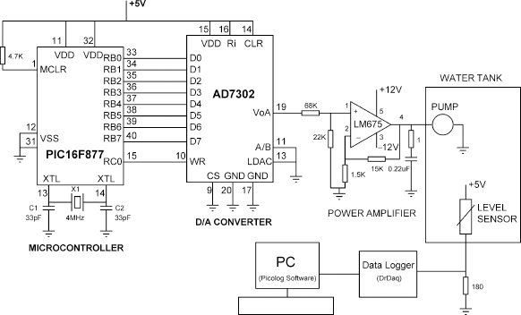
Figure 11.6 Hardware set-up to record the step response
The microcontroller program to send a step signal to the D/A converter is shown in Figure 11.7. At the beginning of the program the input–output ports are configured and then a step signal (200) is sent to port B. The D/A converter is then enabled by clearing its WR input. After writing data to the D/A converter it is disabled so that its output does not accidentally change. The program then waits in an endless loop.
Figure 11.8 shows the step response of the system, which is the response of a typical first-order system. It will be seen that the response contains noise. Also, since the DrDaq data logger is 8-bit, its resolution is about 19.5 mV with a reference input of 5V, and this causes the step discontinuities shown in the response (the steps can be eliminated either by using a data logger with a higher resolution, or by amplifying the output of the level sensor). The figure clearly shows that in practice the response of a system is not always a perfect textbook signal.
A smooth curve is drawn through the response by taking the midpoints of the steps, as shown in Figure 11.9.
11.4 DESIGNING A CONTROLLER
The circuit diagram of the closed-loop system is shown in Figure 11.10. The loop is closed by connecting the output of the level sensor to the analog input AN0 of the microcontroller.

Figure 11.7 Microcontroller program to send a step to D/A
A controller algorithm was then implemented in the microcontroller to control the level of the water in the tank.
One of the requirements in this case study is zero steady-state error, which can be achieved by having an integral type controller. In this case study a Ziegler–Nichols PI controller was designed.
The system model can be derived from the step response. As shown in Figure 11.11, the Ziegler–Nichols system model parameters are given by T1 = 31 s, TD =2s and
![]()
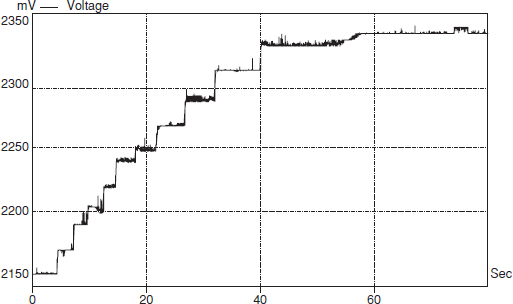
Figure 11.8 System step response
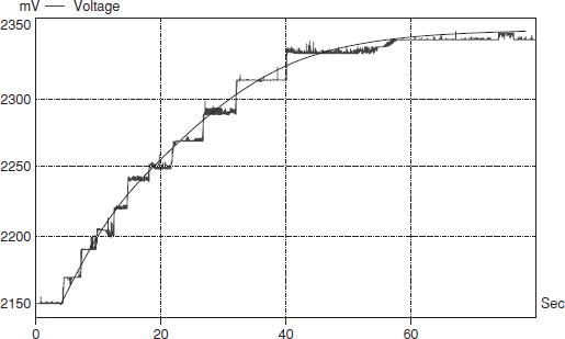
Figure 11.9 Step response after smoothing the curve
Notice that the output of the microcontroller was set to 200, which corresponds to 200×5000/256 = 3906 mV, and this was the voltage applied to the power. We then obtain the following transfer function:
![]()
The time constant of the system is 31 s. It was shown in Section 10.6 that the sampling time should be chosen to be less than one-tenth of the system time constant, i.e. T < 3.1s. In this case study, the sampling time is chosen to be 100 ms, i.e. T = 0.1s.

Figure 11.10 Circuit diagram of the closed-loop system

Figure 11.11 Deriving the system model

Figure 11.12 Realization of the controller
The coefficients of a Ziegler–Nichols PI controller were given in Chapter 10:
![]()
Thus, the PI parameters of our system are:
![]()
A parallel PI controller was realized in this case study. The controller is in the form of (10.27), with the derivative term set to zero, i.e.
![]()
The realization of the controller as a parallel structure is shown in Figure 11.12.
The controller software is shown in Figure 11.13. The PI algorithm has been implemented as a parallel structure. At the beginning of the program the controller parameters are defined. The program consists of the functions Initialize_AD, Initialize_Timer, Read_AD_Input, and the interrupt service routine (ISR). The A/D converter is initialized to receive analog data from channel AN0. The Read_AD_Input function reads a sample from the A/D converter and stores it in variable yk. The timer is initialized to interrupt every 10 ms. At the beginning of the ISR routine, the PI algorithm is implemented after every 10th interrupt, i.e. every 100 ms. This ensures that the controller sampling time is 100 ms. The ISR routine reads the output of the level sensor and converts it to digital. Then the PI controller algorithm is implemented. Notice that in the algorithm the input of the D/A converter is limited to full scale, i.e. 255. After sending an output to D/A, the ISR routine re-enables the timer interrupts and the program waits for the occurrence of the next interrupt.
The step response of the closed-loop system is shown in Figure 11.14. Here, the reference input was set to 2280. Clearly the system response, although noisy, reaches the set-point with no steady-state error, as desired.
11.5 CONCLUSIONS
Although the case study given in this chapter is simple, it illustrates the basic principles of designing a digital controller, from the identification of the system to the implementation of a suitable controller algorithm on a microcontroller. Here the classical Ziegler–Nichols PI type controller has been implemented. The Ziegler–Nichols tuning method is based on a quarter-amplitude decay ratio, which means that the amplitude of an oscillation is reduced by a factor of 4 over a whole period. This corresponds to a damping ratio of about 0.2, which gives rise to a large overshoot. Ziegler–Nichols tuning method has been very popular and most manufacturers of controllers have used these rules with some modifications. The biggest advantage of the Ziegler–Nichols tuning method is its simplicity.

Figure 11.13 Software of the controller
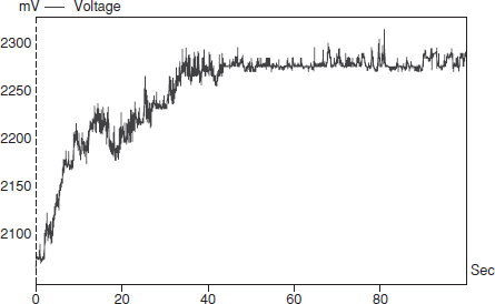
Figure 11.14 Step response of the closed-loop system
In practice one has to consider various implementation-related problems, such as:
- integral wind-up of the PID controller;
- the derivative kick of the PID controller;
- quantization errors produced as a result of the finite word-length data storage and finite word-length arithmetic;
- errors produced as a result of the finite word length of the A/D and the D/A converters.
Quantization errors are an important topic in the design of digital controllers using microcontrollers and programming languages with fixed-point arithmetic. Numbers have to be approximated in order to fit the word length of the digital computer used. Approximations occur at the A/D conversion stage. The A/D converter represents +5V with 8, 12 or 16 bits. The resolution is then 19.53 mV for an 8-bit converter, 4.88 mV for a 12-bit converter, and 0.076 mV for a 16-bit converter. If, for example, we are using an 8-bit A/D converter then a signal change less than 19.53 mV will not be recognized by the system.
Approximations also occur at the D/A conversion stage where the output of the digital algorithm has to be converted into an analog signal to drive the plant. The finite resolution of the D/A converter introduces errors into the algorithm.
Quantization errors occur after the mathematical operations inside the microcontroller, especially after a multiplication where the result must be truncated or rounded before being stored.
Controller parameters are not integers, and quantization errors occur when these constants are introduced into the controller algorithm.
When floating-point arithmetic is used (e.g. when using C language) in 8-bit microcontrollers, numbers can be stored with very high accuracy. The effects of the quantization errors due to mathematical operations inside the microcontroller are very small in such applications. The errors due to the finite resolution of the A/D and D/A converters can still introduce errors into the system and cause unexpected behaviour.