9

Discrete Controller Design

The design of a digital control system begins with an accurate model of the process to be controlled. Then a control algorithm is developed that will give the required system response. The loop is closed by using a digital computer as the controller. The computer implements the control algorithm in order to achieve the required response.

Several methods can be used for the design of a digital controller:

• A system transfer function is modelled and obtained in the s-plane. The transfer function is then transformed into the z-plane and the controller is designed in the z-plane.
• System transfer function is modelled as a digital system and the controller is directly designed in the z-plane.
• The continuous system transfer function is transformed into the w-plane. A suitable controller is then designed in the w-plane using the well-established time response (e.g. root locus) or frequency response (e.g. Bode diagram) techniques. The final design is transformed into the z-plane and the algorithm is implemented on the digital computer.

In this chapter we are mainly interested in the design of a digital controller using the first method, i.e. the controller is designed directly in the z-plane.

The procedure for designing the controller in the z-plane can be outlined as follows:

• Derive the transfer function of the system either by using a mathematical approach or by performing a frequency or a time response analysis.
• Transform the system transfer function into the z-plane.
• Design a suitable digital controller in the z-plane.
• Implement the controller algorithm on a digital computer.

A discrete-time system can be in many different forms, depending on the type of input and the type of sensor used. Figure 9.1 shows a discrete-time system where the reference input is an analog signal, and the process output is also an analog signal. Analog-to-digital converters are then used to convert these signals into digital form so that they can be processed by a digital computer. A zero-order hold at the output of the digital controller approximates a D/A converter which produces an analog signal to drive the plant.

In Figure 9.2 the reference input is a digital signal, which is usually set using a keyboard or can be hard-coded into the controller algorithm. The feedback signal is also digital and the error signal is formed by the computer after subtracting the feedback signal from the reference input. The digital controller then implements the control algorithm and derives the plant.

Figure 9.1 Discrete-time system with analog reference input

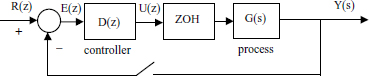
Figure 9.2 Discrete-time system with digital reference input

9.1 DIGITAL CONTROLLERS

In general, we can make use of the block diagram shown in Figure 9.3 when designing a digital controller. In this figure, R(z) is the reference input, E(z) is the error signal, U(z) is the output of the controller, and Y(z) is the output of the system. HG(z) represents the digitized plant transfer function together with the zero-order hold.

The closed-loop transfer function of the system in Figure 9.3 can be written as

Now, suppose that we wish the closed-loop transfer function to be T(z), i.e.

Then the required controller that will give this closed-loop response can be found by using (9.1) and (9.2):

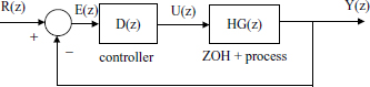
Figure 9.3 Discrete-time system

Equation (9.3) states that the required controller D(z) can be designed if we know the model of the process. The controller D(z) must be chosen so that it is stable and can be realized. One of the restrictions affecting realizability is that D(z) must not have a numerator whose order exceeds that of the numerator. Some common controllers based on (9.3) are described below.

9.1.1 Dead-Beat Controller

The dead-beat controller is one in which a step input is followed by the system but delayed by one or more sampling periods, i.e. the system response is required to be equal to unity at every sampling instant after the application of a unit step input.

The required closed-loop transfer function is then

From (9.3), the required digital controller transfer function is

An example design of a controller using the dead-beat algorithm is given below.

Example 9.1

The open-loop transfer function of a plant is given by

Design a dead-beat digital controller for the system. Assume that T =1s.

Solution

The transfer function of the system with a zero-order hold is given by

or

From z-transform tables we obtain

or

From Equations (9.3) and (9.5),

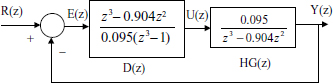
Figure 9.4 Block diagram of the system of Example 9.1

For realizability, we can choose k ≥ 3. Choosing k = 3, we obtain

or

Figure 9.4 shows the system block diagram with the controller, while Figure 9.5 shows the step response of the system. The output response is unity after 3 s (third sample) and stays at this value. It is important to realize that the response is correct only at the sampling instants and the response can have an oscillatory behaviour between the sampling instants.

The control signal applied to the plant is shown in Figure 9.6. Although the dead-beat controller has provided an excellent response, the magnitude of the control signal may not be acceptable, and it may even saturate in practice.

Figure 9.5 Step response of the system

Figure 9.6 Control signal

The dead-beat controller is very sensitive to plant characteristics and a small change in the plant may lead to ringing or oscillatory response.

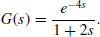
9.1.2 Dahlin Controller

The Dahlin controller is a modification of the dead-beat controller and produces an exponential response which is smoother than that of the dead-beat controller.

The required response of the system in the s-plane can be shown to be

where a and q are chosen to give the required response (see Figure 9.7). If we let a = kT, then the z-transform of the output is

and the required transfer function is

Figure 9.7 Dahlin controller response

or

Using (9.3), we can find the transfer function of the required controller:

An example is given below to illustrate the use of the Dahlin controller.

Example 9.2

The open-loop transfer function of a plant is given by

Design a Dahlin digital controller for the system. Assume that T =1s.

Solution

The transfer function of the system with a zero-order hold is given by

or

From z-transform tables we obtain

or

Figure 9.8 System response with Dahlin controller

For the controller, if we choose q = 10, then

or

For realizability, if we choose k = 2, we obtain

Figure 9.8 shows the step response of the system. It is clear that the response is exponential as expected.

The response of the controller is shown in Figure 9.9. Although the system response is slower, the controller signal is more acceptable.

9.1.3 Pole-Placement Control – Analytical

The response of a system is determined by the positions of its closed-loop poles. Thus, by placing the poles at the required points we should be able to control the response of a system.

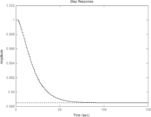
Figure 9.9 Controller response

Given the pole positions of a system, (9.3) gives the required transfer function of the controller as

T(z) is the required transfer function, which is normally in the form of a polynomial. The denominator of T(z) is constructed from the positions of the required roots. The numerator polynomial can then be selected to satisfy certain criteria in the system. An example is given below.

Example 9.3

The open-loop transfer function of a system together with a zero-order hold is given by

Design a digital controller so that the closed-loop system will have ζ = 0.6 and w_d = 3 rad/s. The steady-state error to a step input should be zero. Also, the steady-state error to a ramp input should be 0.2. Assume that T = 0.2s.

Solution

The roots of a second-order system are given by

Thus, the required pole positions are

z_1,2 = e^{−0.6×3.75×0.2}(cos(0.2 × 3) ± j sin(0.2 × 3)) = 0.526 ± j0.360.

The required controller then has the transfer function

which gives

We now have to determine the parameters of the numerator polynomial. To ensure realizability, b₀ = 0 and the numerator must only have the b₁ and b₂ terms. Equation (9.6) then becomes

The other parameters can be determined from the steady-state requirements.

The steady-state error is given by

For a unit step input, the steady-state error can be determined from the final value theorem, i.e.

or

From (9.8), for a zero steady-state error to a step input,

From (9.7), we have

or

If K_v is the system velocity constant, for a steady-state error to a ramp input we can write

or, using L‘Hospital’s rule,

Thus from (9.10),

giving

or

From (9.9) and (9.11) we obtain,

Equation (9.10) then becomes

Equation (9.12) is the required transfer function. We can substitute in Equation (9.3) to find the transfer function of the controller:

or

which can be written as

The step response of the system with the controller is shown in Figure 9.10.

9.1.4 Pole-Placement Control – Graphical

In the previous subsection we saw how the response of a closed-loop system can be shaped by placing its poles at required points in the z-plane. In this subsection we will be looking at some examples of pole placement using the root-locus graphical approach.

When it is required to place the poles of a system at required points in the z-plane we can either modify the gain of the system or use a dynamic compensator (such as a phase lead or a phase lag). Given a first-order system, we can modify only the d.c. gain to achieve the required time constant. For a second-order system we can generally modify the d.c. gain to achieve a constant damping ratio greater than or less than a required value, and, depending on the system, we may also be able to design for a required natural frequency by simply varying the d.c. gain. For more complex requirements, such as placing the system poles at specific points in the z-plane, we will need to use dynamic compensators, and a simple gain adjustment alone will not be adequate. Some example pole-placement techniques are given below using the root locus approach.

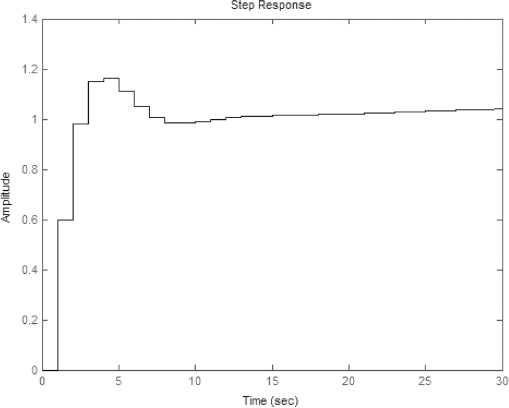
Figure 9.10 Step response of the system

Example 9.4

The block diagram of a sampled data control system is shown in Figure 9.11. Find the value of d.c. gain K which yields a damping ratio of ζ = 0.7.

Solution

In this example, we will draw the root locus of the system as the gain K is varied, and then we will superimpose the lines of constant damping ratio on the locus. The value of K for the required damping ratio can then be read from the locus.

The root locus of the system is shown in Figure 9.12. The locus has been expanded for clarity between the real axis points (−1, 1) and the imaginary axis points (−1, 1), and the lines of constant damping ratio are shown in Figure 9.13. A vertical and a horizontal line are drawn from the point where the damping factor is 0.7. At the required point the roots are z_1,2 = 0.7191 ± j0.2114. The value of K at this point is calculated to be K = 0.0618.

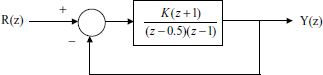
Figure 9.11 Block diagram for Example 9.4

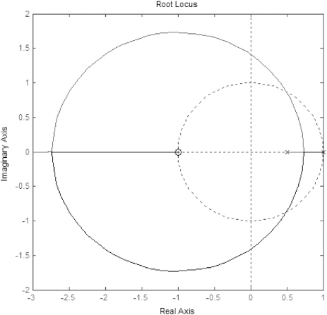
Figure 9.12 Root locus of the system

Figure 9.13 Root locus with the lines of constant damping ratio

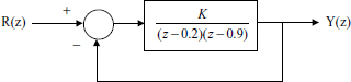
Figure 9.14 Block diagram for Example 9.5

In this example, the required specification was obtained by simply modifying the d.c. gain of the system. A more complex example is given below where it is required to place the poles at specific points in the z-plane.

Example 9.5

The block diagram of a digital control system is given in Figure 9.14. It is required to design a controller for this system such that the system poles are at the points z_1,2 = 0.3 ± j0.3.

Solution

In this example, we will draw the root locus of the system and then use a dynamic compensator to modify the shape of the locus so that it passes through the required points in the z-plane.

The root locus of the system without the compensator is shown in Figure 9.15. The point where we want the roots to be is marked with a × and clearly the locus will not pass through this point by simply modifying the d.c. gain K of the system.

The angle of G(z) at the required point is

or

Since the sum of the angles at a point in the root locus must be a multiple of −180°, the compensator must introduce an angle of −180− (−45) = −135°. The required angle can be obtained using a compensator with a transfer function

The angle introduced by the compensator is

or

There are many combinations of p and n which will give the required angle. For example, if we choose n = 0.5, then,

Figure 9.15 Root locus of the system without compensator

or

The required controller transfer function is then

The compensator introduces a zero at z = 0.5 and a pole at z = 0.242. The root locus of the compensated system is shown in Figure 9.16. Clearly the new locus passes through the required points z_1,2 = 0.3 ± j0.3, and it will be at these points that the d.c. gain is K = 0.185. The step response of the system with the compensator is shown in Figure 9.17. It is clear from this diagram that the system has a steady-state error.

The block diagram of the controller and the system is given in Figure 9.18.

Example 9.6

The block diagram of a system is as shown in Figure 9.19. It is required to design a controller for this system with percent overshoot (PO) less than 17 % and settling time t_s ≤ 10 s. Assume that T = 0.1s.

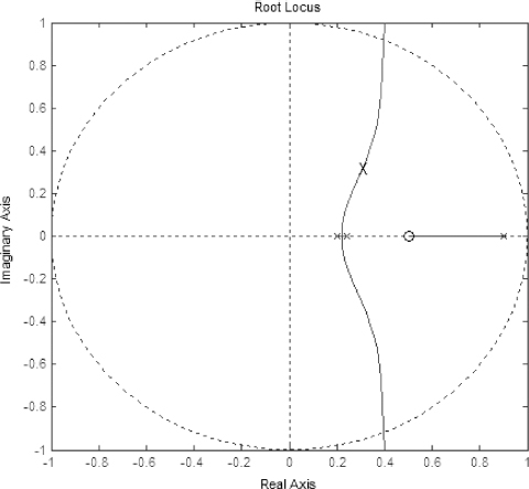
Figure 9.16 Root locus of the compensated system

Figure 9.17 Step response of the system

Figure 9.18 Block diagram of the controller and the system

Figure 9.19 Block diagram for Example 9.6

Solution

The damping ratio, natural frequency and hence the required root positions can be determined as follows:

Hence, the required pole positions are found to be

or

The z-transform of the plant, together with the zero-order hold, is given by

The root locus of the uncompensated system and the required root position is shown in Figure 9.20.

It is clear from the figure that the root locus will not pass through the marked point by simply changing the d.c. gain. We can design a compensator as in Example 9.5 such that the locus passes through the required point, i.e.

The angle of G(z) at the required point is

or

Figure 9.20 Root locus of uncompensated system

Since the sum of the angles at a point in root locus must be a multiple of −180°, the compensator must introduce an angle of −180− (−259) = 79°. The required angle can be obtained using a compensator with a transfer function, and the angle introduced by the compensator is

or

If we choose n = 0.6, then

or

The transfer function of the compensator is thus

Figure 9.21 Root locus of the compensated system

Figure 9.21 shows the root locus of the compensated system. Clearly the locus passes through the required point. The d.c. gain at this point is K = 123.9.

The time response of the compensated system is shown in Figure 9.22.

9.2 PID CONTROLLER

The proportional–integral–derivative (PID) controller is often referred to as a ‘three-term’ controller. It is currently one of the most frequently used controllers in the process industry. In a PID controller the control variable is generated from a term proportional to the error, a term which is the integral of the error, and a term which is the derivative of the error.

• Proportional: the error is multiplied by a gain K_p. A very high gain may cause instability, and a very low gain may cause the system to drift away.
• Integral: the integral of the error is taken and multiplied by a gain K_i. The gain can be adjusted to drive the error to zero in the required time. A too high gain may cause oscillations and a too low gain may result in a sluggish response.
• Derivative: The derivative of the error is multiplied by a gain K_d. Again, if the gain is too high the system may oscillate and if the gain is too low the response may be sluggish.

Figure 9.23 shows the block diagram of the classical continuous-time PID controller. Tuning the controller involves adjusting the parameters K_p, K_d and K_i in order to obtain a satisfactory response. The characteristics of PID controllers are well known and well established, and most modern controllers are based on some form of PID.

Figure 9.22 Time response of the system

Figure 9.23 Continuous-time system PID controller

The input–output relationship of a PID controller can be expressed as

where u(t) is the output from the controller and e(t) = r(t)− y(t), in which r(t) is the desired set-point (reference input) and y(t) is the plant output. T_i and T_d are known as the integral and derivative action time, respectively. Notice that (9.14) is sometimes written as

where

Taking the Laplace transform of (9.14), we can write the transfer function of a continuous-time PID as

To implement the PID controller using a digital computer we have to convert (9.14) from a continuous to a discrete representation. There are several methods for doing this and the simplest is to use the trapezoidal approximation for the integral and the backward difference approximation for the derivative:

Equation (9.14) thus becomes

The PID given by (9.18) is now in a suitable form which can be implemented on a digital computer. This form of the PID controller is also known as the positional PID controller. Notice that a new control action is implemented at every sample time.

The discrete form of the PID controller can also be derived by finding the z-transform of (9.17):

Expanding (9.19) gives

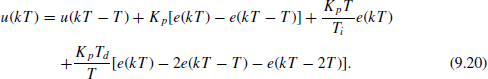
This form of the PID controller is known as the velocity PID controller. Here the current control action uses the previous control value as a reference. Because only a change in the control action is used, this form of the PID controller provides a smoother bumpless control when the error is small. If a large error exists, the response of the velocity PID controller may be slow, especially if the integral action time T_i is large.

The two forms of the PID algorithm, (9.18) and (9.20), may look quite different, but they are in fact similar to each other. Consider the positional controller (9.18). Shifting back one sampling interval, we obtain

Subtracting from (9.18), we obtain the velocity form of the controller, as given by (9.20).

9.2.1 Saturation and Integral Wind-Up

In practical applications the output value of a control action is limited by physical constraints. For example, the maximum voltage output from a device is limited. Similarly, the maximum flow rate that a pump can supply is limited by the physical capacity of the pump. As a result of this physical limitation, the error signal does not return to zero and the integral term keeps adding up continuously. This effect is called integral wind-up (or integral saturation), and as a result of it long periods of overshoot can occur in the plant response. A simple example of what happens is the following. Suppose we wish to control the position of a motor and a large setpoint change occurs, resulting in a large error signal. The controller will then try to reduce the error between the set-point and the output. The integral term will grow by summing the error signals at each sample and a large control action will be applied to the motor. But because of the physical limitation of the motor electronics the motor will not be able to respond linearly to the applied control signal. If the set-point now changes in the other direction, then the integral term is still large and will not respond immediately to the set-point request. Consequently, the system will have a poor response when it comes out of this condition.

The integral wind-up problem affects positional PID controllers. With velocity PID controllers, the error signals are not summed up and as a result integral wind-up will not occur, even though the control signal is physically constrained.

Many techniques have been developed to eliminate integral wind-up from the PID controllers, and some of the popular ones are as follows:

• Stop the integral summation when saturation occurs. This is also called conditional integration. The idea is to set the integrator input to zero if the controller output is saturated and the input and output are of the same sign.
• Fix the limits of the integral term between a minimum and a maximum.
• Reduce the integrator input by some constant if the controller output is saturated. Usually the integral value is decreased by an amount proportional to the difference between the unsaturated and saturated (i.e maximum) controller output.
• Use the velocity form of the PID controller.

9.2.2 Derivative Kick

Another possible problem when using PID controllers is caused by the derivative action of the controller. This may happen when the set-point changes sharply, causing the error signal to change suddenly. Under such a condition, the derivative term can give the output a kick, known as a derivative kick. This is usually avoided in practice by moving the derivative term to the feedback loop. The proportional term may also cause a sudden kick in the output and it is common to move the proportional term to the feedback loop.

9.2.3 PID Tuning

When a PID controller is used in a system it is important to tune the controller to give the required response. Tuning a PID controller involves selecting values for the controller parameters K_p, T_i and T_d. There are many techniques for tuning a controller, ranging from the first techniques described by J.G. Ziegler and N.B. Nichols (known as the Ziegler–Nichols tuning algorithm) in 1942 and 1943, to recent auto-tuning controllers. In this section we shall look at the tuning of PID controllers using the Ziegler–Nichols tuning algorithm.

Ziegler and Nichols suggested values for the PID parameters of a plant based on open-loop or closed-loop tests of the plant. According to Ziegler and Nichols, the open-loop transfer function of a system can be approximated with a time delay and a single-order system, i.e.

where T_D is the system time delay (i.e. transportation delay), and T₁ is the time constant of the system.

9.2.3.1 Open-Loop Tuning

For open-loop tuning, we first find the plant parameters by applying a step input to the open-loop system. The plant parameters K, T_D and T₁ are then found from the result of the step test as shown in Figure 9.24.

Ziegler and Nichols then suggest using the PID controller settings given in Table 9.1 when the loop is closed. These parameters are based on the concept of minimizing the integral of the absolute error after applying a step change to the set-point.

An example is given below to illustrate the method used.

Figure 9.24 Finding plant parameters K, T_D and T₁

Table 9.1 Open-loop Ziegler–Nichols settings

Example 9.7

The open-loop unit step response of a thermal system is shown in Figure 9.25. Obtain the transfer function of this system and use the Ziegler–Nichols tuning algorithm to design (a) a proportional controller, (b) to design a proportional plus integral (PI) controller, and (c) to design a PID controller. Draw the block diagram of the system in each case.

Solution

From Figure 9.25, the system parameters are obtained as K = 40°C, T_D =5s and T₁ = 20 s, and the transfer function of the plant is

Proportional controller. According to Table 9.1, the Ziegler–Nichols settings for a proportional controller are:

Thus,

Figure 9.25 Unit step response of the system for Example 9.7

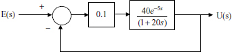
Figure 9.26 Block diagram of the system with proportional controller

The transfer function of the controller is then

and the block diagram of the closed-loop system with the controller is shown in Figure 9.26.

PI controller. According to Table 9.1, the Ziegler–Nichols settings for a PI controller are

Thus,

The transfer function of the controller is then

and the block diagram of the closed-loop system with the controller is shown in Figure 9.27.

PID controller. According to Table 9.1, the Ziegler–Nichols settings for a PID controller are

Thus,

The transfer function of the required PID controller is

or

The block diagram of the system, together with the controller, is shown in Figure 9.28.

Figure 9.27 Block diagram of the system with PI controller

Figure 9.28 Block diagram of the system with PID controller

9.2.3.2 Closed-Loop Tuning

The Ziegler–Nichols closed-loop tuning algorithm is based on plant closed-loop tests. The procedure is as follows:

• Disable any derivative and integral action in the controller and leave only the proportional action.
• Carry out a set-point step test and observe the system response.
• Repeat the set-point test with increased (or decreased) controller gain until a stable oscillation is achieved (see Figure 9.29). This gain is called the ultimate gain, K_u.
• Read the period of the steady oscillation and let this be P_u.
• Calculate the controller parameters according to the following formulae: K_p = 0.45K_u, T_i = P_u/1.2 in the case of the PI controller; and K_p = 0.6K_u, T_i = P_u/2, T_d = T_u/8 in the case of the PID controller.

9.3 EXERCISES

1. The open-loop transfer function of a plant is given by:

   

   (a) Design a dead-beat digital controller for the system. Assume that T =1s.

   (b) Draw the block diagram of the system together with the controller.

   (c) Plot the time response of the system.

   

   Figure 9.29 Ziegler–Nichols closed-loop test

2. Repeat Exercise 1 for a Dahlin controller. Plot the response and compare with the results obtained from the dead-beat controller.
3. The open-loop transfer function of a system together with a zero-order hold is given by

   

   Design a digital controller so that the closed-loop system will have ζ = 0.6 and w_d = 3 rad/s. The steady-state error to a step input should be zero. Also, the steady state error to a ramp input should be 0.5. Assume that T = 0.2s.

4. The block diagram of a sampled data control system is shown in Figure 9.30. Find the value of d.c. gain K to yield a damping ratio of 0.6
5. Draw the time response of the system in Exercise 4.
6. The open-loop transfer function of a system is

   

   The system is preceded by a sampler and a zero-order hold. The closed-loop system is required to have a time constant of 0.4 s. (a) Determine the required value of the d.c. gain K. (b) Plot the unit step time response of the system with the controller.

7. The block diagram of a system is given in Figure 9.31. It is required to design a controller for this system such that the system poles are at the points z_1,2 = 0.4 ± j0.4inthe z-plane. (a) Derive the transfer function of the required digital controller. (b) Plot the unit step time response of the system without the controller. (c) Plot the unit step time response of the system with the controller.
8. The block diagram of a system is given in Figure 9.32. It is required to design a controller for this system with percent overshoot (PO) less than 20 % and settling time t_s ≤ 10 s. Assume that the sampling time is, T = 0.1s.

   (a) Derive the transfer function of the required digital controller.

   (b) Draw the block diagram of the system together with the controller.

   (c) Plot the unit step time response of the system without the controller.

   

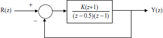
   Figure 9.30 Block diagram for Exercise 4

   

   Figure 9.31 Block diagram for Exercise 7

   

   Figure 9.32 Block diagram for Exercise 8

   (d) Plot the unit step time response of the system with the controller.

9. Explain the differences between the position and velocity forms of the PID controller.
10. The open-loop unit step response of a system is shown in Figure 9.33. Obtain the transfer function of this system and use the Ziegler–Nichols tuning algorithm to design:

    (a) a proportional controller;

    (b) a PI controller;

    (c) a PID controller.

    Draw the block diagram of the system in each case.

11. Explain the procedure for designing a PID controller using the Ziegler–Nichols algorithm when the plant is open-loop.
12. Repeat Exercise 11 for the case when the plant is closed-loop. What precautions should be taken when tests are performed on a closed-loop system?
13. Explain what integral wind-up is when a PID controller is used. How can integral wind-up be avoided?
14. Explain what derivative kick is when a PID controller is used. How can derivative kick be avoided?
15. The open-loop transfer function of a unity feedback system is

    

    

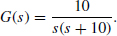
    Figure 9.33 Unit step response of the system for Exercise 10

    

    Figure 9.34 Block diagram for Exercise 17

    Assume that T =1s and design a controller so that the system response to a unit step input is

    

16. A mechanical process has the transfer function Ke^−sTD/s The system oscillates with a frequency of 0.05 Hz when a unity gain feedback is applied. Determine the value of T_D.
17. The block diagram of a system is given in Figure 9.34. It is required to design a controller for this system with percent overshoot (PO) less than 15 % and settling time t_s ≤ 10 s. Assume that the sampling time is, T = 0.2s.

    (a) Derive the transfer function of the required digital controller.

    (b) Draw the block diagram of the system together with the controller.

    (c) Plot the unit step time response of the system without the controller.

    (d) Plot the unit step time response of the system with the controller.

18. Derive an expression for the z-transform model of the continuous-time PID controller. Draw the block diagram of the controller. Describe how you can modify the model to avoid derivative kick.
19. The continuous-time PI controller has the transfer function

    

    Derive the equivalent discrete-time controller transfer function using the bilinear transformation.

20. A commonly used compensator in the s-plane is the lead lag, or lag lead with transfer function

    

    Find the equivalent discrete-time controller using the bilinear transformation.

FURTHER READING

[Dorf, 1974] Dorf, R.C. Modern Control Systems. Addison-Wesley Reading, MA, 1974.

[Franklin et al., 1990] Franklin, G.F., Powell, J.D., and Workman, M.L. Digital Control of Dynamic Systems. 2nd edn., Addison-Wesley, Reading, MA, 1990.

[Katz, 1981] Katz, P. Digital Control Using Microprocessors. Prentice Hall International, Engle wood Cliffs, NJ, 1981.

[Kuo, 1963] Kuo, B.C. Analysis and Synthesis of Sampled-Data Control Systems. Prentice Hall International, Eaglewood Cliffs, NJ, 1963.

[Ogata, 1970] Ogata, K. Modern Control Engineering. McGraw-Hill, New York, 1970.

[Phillips and Harbor, 1988] Phillips, C.L. and Harbor, R.D. Feedback Control Systems. Prentice Hall, Eaglewood Cliffs, NJ, 1988.

[Strum and Kirk, 1988] Strum, R.D. and Kirk, D.E. Discrete Systems and Digital Signal Processing. Addison Wesley, Reading, MA, 1988.

[Tustin, 1947] Tustin, A. A method of analyzing the behaviour of linear systems in terms of time series. J. Inst. Elect. Engineers. 94, Pt. IIA, 1947, pp. 130–142.