6

Sampled Data Systems and the z-Transform

A sampled data system operates on discrete-time rather than continuous-time signals. A digital computer is used as the controller in such a system. A D/A converter is usually connected to the output of the computer to drive the plant. We will assume that all the signals enter and leave the computer at the same fixed times, known as the sampling times.

A typical sampled data control system is shown in Figure 6.1. The digital computer performs the controller or the compensation function within the system. The A/D converter converts the error signal, which is a continuous signal, into digital form so that it can be processed by the computer. At the computer output the D/A converter converts the digital output of the computer into a form which can be used to drive the plant.

6.1 THE SAMPLING PROCESS

A sampler is basically a switch that closes every T seconds, as shown in Figure 6.2. When a continuous signal r(t) is sampled at regular intervals T, the resulting discrete-time signal is shown in Figure 6.3, where q represents the amount of time the switch is closed.

In practice the closure time q is much smaller than the sampling time T, and the pulses can be approximated by flat-topped rectangles as shown in Figure 6.4.

In control applications the switch closure time q is much smaller than the sampling time T and can be neglected. This leads to the ideal sampler with output as shown in Figure 6.5.

The ideal sampling process can be considered as the multiplication of a pulse train with a continuous signal, i.e.

where P(t) is the delta pulse train as shown in Figure 6.6, expressed as

thus,

Figure 6.1 Sampled data control system

Figure 6.2 A sampler

Figure 6.3 The signal r(t) after the sampling operation

Figure 6.4 Sampled signal with flat-topped pulses

Figure 6.5 Signal r(t) after ideal sampling

Figure 6.6 Delta pulse train

or

Now

and

Taking the Laplace transform of (6.6) gives

Equation (6.7) represents the Laplace transform of a sampled continuous signal r(t).

A D/A converter converts the sampled signal r*(t) into a continuous signal y(t). The D/A can be approximated by a zero-order hold (ZOH) circuit as shown in Figure 6.7. This circuit remembers the last information until a new sample is obtained, i.e. the zero-order hold takes the value r(nT) and holds it constant for nT ≤ t < (n + 1)T, and the value r(nT) is used during the sampling period.

The impulse response of a zero-order hold is shown in Figure 6.8. The transfer function of a zero-order hold is given by

Figure 6.7 A sampler and zero-order hold

Figure 6.8 Impulse response of a zero-order hold

where H(t) is the step function, and taking the Laplace transform yields

A sampler and zero-order hold can accurately follow the input signal if the sampling time T is small compared to the transient changes in the signal. The response of a sampler and a zero-order hold to a ramp input is shown in Figure 6.9 for two different values of sampling period.

Figure 6.9 Response of a sampler and a zero-order hold for a ramp input

Figure 6.10 Ideal sampler and zero-order hold for Example 6.1

Figure 6.11 Solution for Example 6.1

Example 6.1

Figure 6.10 shows an ideal sampler followed by a zero-order hold. Assuming the input signal r(t) is as shown in the figure, show the waveforms after the sampler and also after the zero-order hold.

Solution

The signals after the ideal sampler and the zero-order hold are shown in Figure 6.11.

6.2 THE z-TRANSFORM

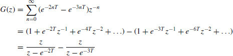
Equation (6.7) defines an infinite series with powers of e^−snT. The z-transform is defined so that

the z-transform of the function r(t) is Z[r(t)] = R(z) which, from (6.7), is given by

Notice that the z-transform consists of an infinite series in the complex variable z, and

i.e. the r(nT) are the coefficients of this power series at different sampling instants.

The z-transformation is used in sampled data systems just as the Laplace transformation is used in continuous-time systems. The response of a sampled data system can be determined easily by finding the z-transform of the output and then calculating the inverse z-transform, just like the Laplace transform techniques used in continuous-time systems. We will now look at how we can find the z-transforms of some commonly used functions.

Figure 6.12 Unit step function

6.2.1 Unit Step Function

Consider a unit step function as shown in Figure 6.12, defined as

From (6.11),

or

6.2.2 Unit Ramp Function

Consider a unit ramp function as shown in Figure 6.13, defined by

From (6.11),

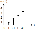
Figure 6.13 Unit ramp function

Figure 6.14 Exponential function

or

6.2.3 Exponential Function

Consider the exponential function shown in Figure 6.14, defined as

From (6.11)

or

6.2.4 General Exponential Function

Consider the general exponential function

From (6.11),

or

Similarly, we can show that

6.2.5 Sine Function

Consider the sine function, defined as

Recall that

so that

But we already know from (6.12) that the z-transform of an exponential function is

Therefore, substituting in (6.13) gives

or

6.2.6 Cosine Function

Consider the cosine function, defined as

Recall that

so that

But we already know from (6.12) that the z-transform of an exponential function is

Therefore, substituting in (6.14) gives

or

6.2.7 Discrete Impulse Function

Consider the discrete impulse function defined as

From (6.11),

6.2.8 Delayed Discrete Impulse Function

The delayed discrete impulse function is defined as

From (6.11),

6.2.9 Tables of z-Transforms

A table of z-transforms for the commonly used functions is given in Table 6.1 (a bigger table is given in Appendix A). As with the Laplace transforms, we are interested in the output response y(t) of a system and we must find the inverse z-transform to obtain y(t) from Y(z).

6.2.10 The z-Transform of a Function Expressed as a Laplace Transform

It is important to realize that although we denote the z-transform equivalent of G(s) by G(z), G(z) is not obtained by simply substituting z for s in G(s). We can use one of the following methods to find the z-transform of a function expressed in Laplace transform format:

• Given G(s), calculate the time response g(t) by finding the inverse Laplace transform of G(s). Then find the z-transform either from the first principles, or by looking at the z-transform tables.
• Given G(s), find the z-tranform G(z) by looking at the tables which give the Laplace transforms and their equivalent z-transforms (e.g. Table 6.1).
• Given the Laplace transform G(s), express it in the form G(s) = N(s)/D(s) and then use the following formula to find the z-transform G(z):

Table 6.1 Some commonly used z-transforms

where D' = ∂D/∂s and the x_n, n = 1,2,..., p, are the roots of the equation D(s) = 0. Some examples are given below.

Example 6.2

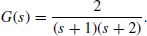
Let

Determine G(s) by the methods described above.

Solution

Method 1: By finding the inverse Laplace transform. We can express G(s) as a sum of its partial fractions:

The inverse Laplace transform of (6.16) is

From the definition of the z-transforms we can write (6.17) as

or

Method 2: By using the z-transform transform tables for the partial product. From Table 6.1, the z-transform of 1/(s + a) is z/(z − e^−aT). Therefore the z-transform of (6.16) is

or

Method 3: By using the z-transform tables for G(s). From Table 6.1, the z-transform of

is

Comparing (6.18) with (6.16) we have, a = 2, b = 3. Thus, in (6.19) we get

Method 4: By using equation (6.15). Comparing our expression

with (6.15), we have N(s) = 1, D(s) = s² + 5s + 6 and D (s) = 2s + 5, and the roots of D(s) = 0 are x₁=−2 and x₂=−3. Using (6.15),

or, when x₁ = −2,

and when x₁ = −3,

Thus,

or

6.2.11 Properties of z-Transforms

Most of the properties of the z-transform are analogs of those of the Laplace transforms. Important z-transform properties are discussed in this section.

1. Linearity property

   Suppose that the z-transform of f (nT) is F(z) and the z-transform of g(nT) is G(z). Then

   

   and for any scalar a

   

2. Left-shifting property

   Suppose that the z-transform of f (nT) is F(z) and let y(nT) = f (nT +mT). Then

   

   If the initial conditions are all zero, i.e. f (iT) = 0, i = 0,1,2,...,m − 1, then,

   

3. Right-shifting property

   Suppose that the z-transform of f (nT) is F(z) and let y(nT) = f (nT −mT). Then

   

   If f (nT) = 0 for k < 0, then the theorem simplifies to

   

4. Attenuation property

   Suppose that the z-transform of f (nT) is F(z). Then,

   

   This result states that if a function is multiplied by the exponential e−^anT then in the z-transform of this function z is replaced by ze^aT.

5. Initial value theorem

   Suppose that the z-transform of f (nT) is F(z). Then the initial value of the time response is given by

   

6. Final value theorem

   Suppose that the z-transform of f (nT) is F(z). Then the final value of the time response is given by

Note that this theorem is valid if the poles of (1− z⁻¹)F(z) are inside the unit circle or at z = 1.

Example 6.3

The z-transform of a unit ramp function r(nT) is

Find the z-transform of the function 5r(nT).

Solution

Using the linearity property of z-transforms,

Example 6.4

The z-transform of trigonometric function r(nT) = sin n w T is

find the z-transform of the function y(nT) = e^−2T sin nW T.

Solution

Using property 4 of the z-transforms,

Thus,

or, multiplying numerator and denominator by e^−4T,

Example 6.5

Given the function

find the final value of g(nT).

Solution

Using the final value theorem,

6.2.12 Inverse z-Transforms

The inverse z-transform is obtained in a similar way to the inverse Laplace transforms. Generally, the z-transforms are the ratios of polynomials in the complex variable z, with the numerator polynomial being of order no higher than the denominator. By finding the inverse z-transform we find the sequence associated with the given z-transform polynomial. As in the case of inverse Laplace transforms, we are interested in the output time response of a system. Therefore, we use an inverse transform to obtain y(t) from Y(z). There are several methods to find the inverse z-transform of a given function. The following methods will be described here:

• power series (long division);
• expanding Y(z) into partial fractions and using z-transform tables to find the inverse transforms;
• obtaining the inverse z-transform using an inversion integral.

Given a z-transform function Y(z), we can find the coefficients of the associated sequence y(nT) at the sampling instants by using the inverse z-transform. The time function y(t) is then determined as

Method 1: Power series. This method involves dividing the denominator of Y(z) into the numerator such that a power series of the form

is obtained. Notice that the values of y(n) are the coefficients in the power series.

Example 6.6

Find the inverse z-transform for the polynomial

Solution

Dividing the denominator into the numerator gives

and the coefficients of the power series are

The required sequence is

Figure 6.15 shows the first few samples of the time sequence y(nT).

Example 6.7

Find the inverse z-transform for Y(z) given by the polynomial

Figure 6.15 First few samples ofy(t)

Solution

Dividing the denominator into the numerator gives

and the coefficients of the power series are

The required sequence is thus

Figure 6.16 shows the first few samples of the time sequence y(nT).

The disadvantage of the power series method is that it does not give a closed form of the resulting sequence. We often need a closed-form result, and other methods should be used when this is the case.

Figure 6.16 First few samples ofy(t)

Method 2: Partial fractions. Similar to the inverse Laplace transform techniques, a partial fraction expansion of the function Y(z) can be found, and then tables of known z-transforms can be used to determine the inverse z-transform. Looking at the z-transform tables, we see that there is usually a z term in the numerator. It is therefore more convenient to find the partial fractions of the function Y(z)/z and then multiply the partial fractions by z to obtain a z term in the numerator.

Example 6.8

Find the inverse z-transform of the function

Solution

The above expression can be written as

The values of A and B can be found by equating like powers in the numerator, i.e.

We find A = −1, B = 1, giving

or

From the z-transform tables we find that

and the coefficients of the power series are

so that the required sequence is

Example 6.9

Find the inverse z-transform of the function

Solution

The above expression can be written as

The values of A, B and C can be found by equating like powers in the numerator, i.e. A(z − 1)(z − 2)+ Bz(z − 2)+Cz(z − 1) ≡ 1

or

giving

The values of the coefficients are found to be A = 0.5, B=−1 and C = 0.5. Thus,

or

Using the inverse z-transform tables, we find

where

the coefficients of the power series are

and the required sequence is

The process of finding inverse z-transforms is aided by considering what form is taken by the roots of Y(z). It is useful to distinguish the case of distinct real roots and that of multiple order roots.

Case I: Distinct real roots. When Y(z) has distinct real roots in the form

then the partial fraction expansion can be written as

and the coefficients A_i can easily be found as

Example 6.10

Using the partial expansion method described above, find the inverse z-transform of

Solution

Rewriting the function as

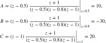
we find that

Thus,

and the inverse z-transform is obtained from the tables as

which is the same answer as in Example 6.7.

Example 6.11

Using the partial expansion method described above, find the inverse z-transform of

Solution

Rewriting the function as

we find that

Thus,

The inverse transform is found from the tables as

The coefficients of the power series are

and the required sequence is

Case II: Multiple order roots. When Y(z) has multiple order roots of the form

then the partial fraction expansion can be written as

and the coefficients λ_i can easily be found as

Example 6.12

Using (6.29), find the inverse z-transform of

Solution

Rewriting the function as

we obtain

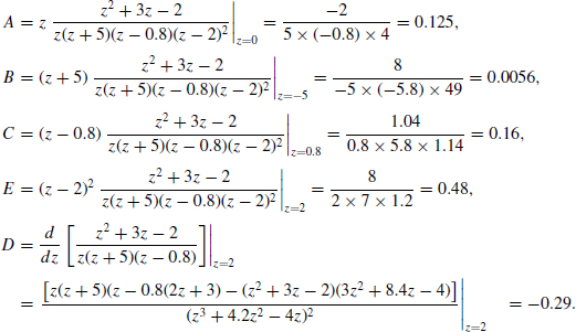
We can now write Y(z) as

The inverse transform is found from the tables as

where

Method 3: Inversion formula method. The inverse z-transform can be obtained using the inversion integral, defined by

Using the theorem of residues, the above integral can be evaluated via the expression

If the function has a simple pole at z = a, then the residue is evaluated as

Example 6.13

Using the inversion formula method, find the inverse z-transform of

Solution

Using (6.31) and (6.32):

which is the same answer as in Example 6.9.

Example 6.14

Using the inversion formula method, find the inverse z-transform of

Solution

Using (6.31) and (6.32),

6.3 PULSE TRANSFER FUNCTION AND MANIPULATION OF BLOCK DIAGRAMS

The pulse transfer function is the ratio of the z-transform of the sampled output and the input at the sampling instants.

Suppose we wish to sample a system with output response given by

Figure 6.17 Sampling a system

as illustrated in Figure 6.17. We sample the output signal to obtain

and

Equations (6.34) and (6.35) tell us that if at least one of the continuous functions has been sampled, then the z-transform of the product is equal to the product of the z-transforms of each function (note that [e*(s)]* = [e*(s)], since sampling an already sampled signal has no further effect). G(z) is the transfer function between the sampled input and the output at the sampling instants and is called the pulse transfer function. Notice from (6.35) that we have no information about the output y(z) between the sampling instants.

6.3.1 Open-Loop Systems

Some examples of manipulating open-loop block diagrams are given in this section.

Example 6.15

Figure 6.18 shows an open-loop sampled data system. Derive an expression for the z-transform of the output of the system.

Solution

For this system we can write

or

and

Example 6.16

Figure 6.19 shows an open-loop sampled data system. Derive an expression for the z-transform of the output of the system.

Figure 6.18 Open-loop system

Figure 6.19 Open-loop system

Solution

The following expressions can be written for the system:

or

and

where

For example, if

and

then from the z-transform tables,

and the output is given by

Example 6.17

Figure 6.20 shows an open-loop sampled data system. Derive an expression for the z-transform of the output of the system.

Figure 6.20 Open-loop system

Solution

The following expressions can be written for the system:

or

and

or

From (6.37) and (6.38),

which gives

For example, if

then

and the output function is given by

or

6.3.2 Open-Loop Time Response

The open-loop time response of a sampled data system can be obtained by finding the inverse z-transform of the output function. Some examples are given below.

Example 6.18

A unit step signal is applied to the electrical RC system shown in Figure 6.21. Calculate and draw the output response of the system, assuming a sampling period of T =1s.

Solution

The transfer function of the RC system is

Figure 6.21 RC system with unit step input

For this system we can write

and

and taking z-transforms gives

The z-transform of a unit step function is

and the z-transform of G(s) is

Thus, the output z-transform is given by

since T =1s and e⁻¹ = 0.368, we get

The output response can be obtained by finding the inverse z-transform of y(z). Using partial fractions,

Calculating A and B, we find that

or

Figure 6.22 RC system output response

From the z-transform tables we find

The first few output samples are

and the output response (shown in Figure 6.22) is given by

It is important to notice that the response is only known at the sampling instants. For example, in Figure 6.22 the capacitor discharges through the resistor between the sampling instants, and this causes an exponential decay in the response between the sampling intervals. But this behaviour between the sampling instants cannot be determined by the z-transform method of analysis.

Example 6.19

Assume that the system in Example 6.17 is used with a zero-order hold (see Figure 6.23). What will the system output response be if (i) a unit step input is applied, and (ii) if a unit ramp input is applied.

Figure 6.23 RC system with a zero-order hold

Solution

The transfer function of the zero-order hold is

and that of the RC system is

For this system we can write

and

or, taking z-transforms,

Now, T =1s and

and by partial fraction expansion we can write

From the z-transform tables we then find that

(i) For a unit step input,

and the system output response is given by

Using the partial fractions method, we can write

where A = 1 and B = −1; thus,

Figure 6.24 Step input time response of Example 6.19

From the inverse z-transform tables we find that the time response is given by

where a is the unit step function; thus

The time response in this case is shown in Figure 6.24.

(ii) For a unit ramp input,

and the system output response (with T = 1) is given by

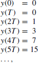
Using the long division method, we obtain the first few output samples as

and the output response is given as

as shown in Figure 6.25.

Example 6.20

The open-loop block diagram of a system with a zero-order hold is shown in Figure 6.26. Calculate and plot the system response when a step input is applied to the system, assuming that T =1s.

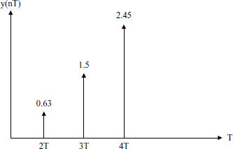
Figure 6.25 Ramp input time response of Example 6.19

Figure 6.26 Open-loop system with zero-order hold

Solution

The transfer function of the zero-order hold is

and that of the plant is

For this system we can write

and

or, taking z-transforms,

Now, T =1s and

or, by partial fraction expansion,

Figure 6.27 Output response

and the z-transform is given by

From the z-transform tables we obtain

After long division we obtain the time response

shown in Figure 6.27.

6.3.3 Closed-Loop Systems

Some examples of manipulating the closed-loop system block diagrams are given in this section.

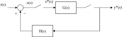
Example 6.21

The block diagram of a closed-loop sampled data system is shown in Figure 6.28. Derive an expression for the transfer function of the system.

Solution

For the system in Figure 6.28 we can write

and

Figure 6.28 Closed-loop sampled data system

Substituting (6.39) into (6.38),

or

and, solving for e*(s), we obtain

and, from (6.39),

The sampled output is then

Writing (6.43) in z-transform format,

and the transfer function is given by

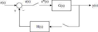
Example 6.22

The block diagram of a closed-loop sampled data system is shown in Figure 6.29. Derive an expression for the output function of the system.

Solution

For the system in Figure 6.29 we can write

Figure 6.29 Closed-loop sampled data system

and

Substituting (6.47) into (6.46), we obtain

or

Solving for y*(s), we obtain

and

Example 6.23

The block diagram of a closed-loop sampled data control system is shown in Figure 6.30. Derive an expression for the transfer function of the system.

Solution

The A/D converter can be approximated with an ideal sampler. Similarly, the D/A converter at the output of the digital controller can be approximated with a zero-order hold. Denoting the digital controller by D(s) and combining the zero-order hold and the plant into G(s), the block diagram of the system can be drawn as in Figure 6.31. For this system can write

Figure 6.30 Closed-loop sampled data system

Figure 6.31 Equivalent diagram for Example 6.23

and

Note that the digital computer is represented as D*(s). Using the above two equations, we can write

or

and, solving for e*(s), we obtain

and, from (6.53),

The sampled output is then

Writing (6.57) in z-transform format,

and the transfer function is given by

Figure 6.32 Closed-loop system

6.3.4 Closed-Loop Time Response

The closed-loop time response of a sampled data system can be obtained by finding the inverse z-transform of the output function. Some examples are given below.

Example 6.24

A unit step signal is applied to the sampled data digital system shown in Figure 6.32. Calculate and plot the output response of the system. Assume that T =1s.

Solution

The output response of this system is given in (6.44) as

where

thus,

Simplifying,

Since T = 1,

After long division we obtain the first few terms

The first 10 samples of the output response are shown in Figure 6.33.

6.4 EXERCISES

1. A function y(t) = 2 sin 4t is sampled every T = 0.1s. Find the z-transform of the resultant number sequence.

   

   Figure 6.33 First 10 output samples

2. Find the z-transform of the function y(t) = 3t.
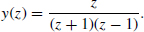
3. Find the inverse z-transform of the function

   

4. The output response of a system is described with the z-transform

   

   (i) Apply the final value theorem to calculate the final value of the output when a unit step input is applied to the system.

   (ii) Check your results by finding the inverse z-transform of y(z).

5. Find the inverse z-transform of the following functions using both long division and the method of partial fractions. Compare the two methods.

   

   

   Figure 6.34 Open-loop system for Exercise 6

   

   Figure 6.35 Open-loop system with zero-order hold for Exercise 10

6. Consider the open-loop system given in Figure 6.34. Find the output response when a unit step is applied, if

   

7. Draw the output waveform of Exercise 6.
8. Find the z-transform of the following function, assuming that T = 0.5s:

   

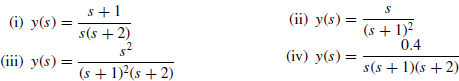
9. Find the z-transforms of the following functions, using z-transform tables:

   

10. Figure 6.35 shows an open-loop system with a zero-order hold. Find the output response when a unit step input is applied. Assume that T = 0.1s and

    

11. Repeat Exercise 10 for the case where the plant transfer function is given by

    

12. Derive an expression for the transfer function of the closed-loop system whose block diagram is shown in Figure 6.36.

    

    Figure 6.36 Closed-loop system for Exercise 12

    

    Figure 6.37 Closed-loop system for Exercise 13

13. Derive an expression for the output function of the closed-loop system whose block diagram is shown in Figure 6.37.

FURTHER READING

[Astrom and Wittenmark, 1984] Astrom, K.J. and Wittenmark, B. Computer Controlled Systems. Prentice Hall, Englewood Cliffs, NJ, 1984.

[D'Azzo and Houpis, 1966] D'Azzo, J.J. and Houpis, C.H. Feedback Control System Analysis and Synthesis, 2nd edn., McGraw-Hill, New York, 1966.

[Dorf, 1992] Dorf, R.C. Modern Control Systems, 6th edn., Addison-Wesley, Reading, MA, 1992.

[Evans, 1954] Evans, W.R. Control System Dynamics. McGraw-Hill, New York, 1954.

[Houpis and Lamont, 1962] Houpis, C.H. and Lamont, G.B. Digital Control Systems: Theory, Hardware, Software, 2nd edn., McGraw-Hill, New York, 1962.

[Hsu and Meyer, 1968] Hsu, J.C. and Meyer, A.U. Modern Control Principles and Applications. McGraw-Hill, New York, 1968.

[Jury, 1958] Jury, E.I. Sampled-Data Control Systems. John Wiley & Sons, Inc., New York, 1958.

[Katz, 1981] Katz, P. Digital Control Using Microprocessors. Prentice Hall, Englewood Cliffs, NJ, 1981.

[Kuo, 1963] Kuo, B.C. Analysis and Synthesis of Sampled-Data Control Systems. Englewood Cliffs, NJ, Prentice Hall, 1963.

[Lindorff, 1965] Lindorff, D.P. Theory of Sampled-Data Control Systems. John Wiley & Sons, Inc., New York, 1965.

[Ogata, 1990] Ogata, K. Modern Control Engineering, 2nd edn., Prentice Hall, Englewood Cliffs, NJ, 1990.

[Phillips and Harbor, 1988] Phillips, C.L. and Harbor, R.D. Feedback Control Systems. Englewood Cliffs, NJ, Prentice Hall, 1988.

[Raven, 1995] Raven, F.H. Automatic Control Engineering, 5th edn., McGraw-Hill, New York, 1995.

[Smith, 1972] Smith, C.L. Digital Computer Process Control. Intext Educational Publishers, Scranton, PA, 1972.

[Strum and Kirk, 1988] Strum, R.D. and Kirk, D.E. First Principles of Discrete Systems and Digital Signal Processing. Addison-Wesley, Reading, MA, 1988.

[Tou, 1959] Tou, J. Digital and Sampled-Data Control Systems. McGraw-Hill, New York, 1959.