
Chapter 2
Modeling and Control of Ionic Polymer-Metal Composite Actuators for Mechatronics Applications 1
This chapter presents the full design process through to the implementation of two innovative mechatronic devices: a stepper motor and a robotic rotary joint both with integrated soft IPMC actuators. Firstly, electromechanical modeling of the IPMC actuation response is presented. This model is then used as a tool for the mechanical design of the devices. Novel implementation of control systems to adaptively handle the highly nonlinear and time-varying response of the IPMCs and achieve successful device performance is undertaken. Experimental results are presented to validate the designs for the systems. This work demonstrates the capabilities of IPMCs and the benefits of implementing them as valid alternatives to traditional actuators.
2.1. Introduction
Ionic polymer-metal composites (IPMCs) are a novel type of smart material transducer. They are a class of electroactive polymer (EAP), acting as an actuator under the influence of an electric field and conversely producing an electric potential when mechanically deformed. Typically IPMCs have been operated in a cantilever configuration (see Figure 2.1) where a voltage is either applied or measured at the base through a set of clamped electrodes. A beam type actuation greater than 90° can be achieved with small applied voltages, typically less than 5 V. Sensing voltage is usually orders of magnitude lower than the voltage for actuation. This chapter focuses on IPMCs operating in actuation mode and their implementation into mechatronics systems.
Figure 2.1. IPMC transducer in cantilever configuration

IPMCs are fabricated with a perfluorinated ionic membrane, for example Nafion® by DuPont, which is sandwiched between two thinly coated conducting electrodes of a noble metal, typically platinum or gold, on either side of the polymer (see Figure 2.2). The ionic polymer must be an ion exchange membrane that is permeable to cations but not anions, consisting of a fixed network of anions with mobile cations.
Figure 2.2. Cross-section of IPMC transducer [AHN 10]

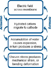
By applying an electric field to the clamped electrodes a voltage is induced across the entire length of the polymer, this attracts the hydrated cations to migrate to the cathode. The accumulation of water on one side of the polymer causes expansion, which in turn produces a stress toward the anode; the uneven stress then produces a mechanical strain, or bending deformation. The opposite effect results in the sensing phenomena in IPMC. The transduction mechanism is summarized in Figure 2.3. In actuation, if a constant electric field is maintained, the actuator will eventually relax back toward the origin as the loose water diffuses back, which is known as “back-relaxation”. Due to the need for hydrated ions, the IPMC operates best in an aqueous environment.
Figure 2.3. Summary of the transduction mechanism for IPMCs
IPMCs are most commonly manufactured in sheets and then individual transducers are cut from the sheet and as such the geometries are infinite and can be tailored to any application requirements. This makes IPMCs highly suited for implementation into any number of mechatronic systems as well as miniaturization in microelectromechanical systems (MEMs) type devices. The IPMC performance characteristics are highly dependent on their geometry; this highlights the importance of developing an accurate scalable model, as presented in the following section, for designing applications with IPMCs.
IPMC materials have a number of superior properties, in comparison with traditional actuators and other EAPs, which make them desirable for use as mechanical actuators, including:
– lightweight and thin, typically between 200 µm and 2 mm thick;
– flexible and compliant, hence safe for operating in sensitive environments;
– low power consumption, hence good for embedded and remote applications;
– achieve both micro- and macro-deflections without any gearing mechanisms [MCD 10c];
– integration of sensing and actuating using the same device;
– low actuation voltages, typically between ±1 and ±5 V;
– biocompatible and implantable in humans [SHA 01a];
– fully operational underwater, at low temperatures and in vacuum [BAR 00b, YE 08];
– completely noiseless actuation, unlike electric motors or pneumatics.
Despite these advantages there are still a number of major issues that need to be overcome before IPMCs can be widely regarded as viable alternatives for traditional actuators.
Some of the major issues include back relaxation under DC actuation, hysteresis, dehydration in air, electrolysis, non-uniform bending, extreme environmental sensitivity (hydration, temperature, humidity level [LAV 05]), and loss of mechanical force at larger displacements. All of these issues imply that the IPMCs are extremely nonlinear (especially at high inputs and low frequencies [SHA 01b, BON 07, MCD 10c]) and time varying.
Over a period of operation the highly time-varying nature of the IPMC will cause the response to change unpredictably. This cannot be fully modeled as the variance is due to ion redistribution which is a stochastic process. This random behavior also makes IPMCs very difficult to accurately control. Robust adaptive control methods must be used to make these systems reliable when operating over a period of time.
Despite the extremely complex nature of IPMCs, modeling is undertaken to give a relatively accurate representation of their response in order to aid in the design of systems and simulate their performance before implementation into real applications. Models alone, however, are not accurate enough over time to be used to develop controllers in simulation.
Some industrial applications which have been explored with IPMCs so far are a micropump [SAN 10], microgripper [YUN 06a], manipulators [HUN 08], vibration reduction [SAG 92], mobile micro-robot [TAK 06], window cleaner [BAR 00a] as well as applications in other areas like robotic finger prosthesis [CHE 09], an assistive heart compression device [SHA 01a], and a snake robot [HUN 08]. While there have been many attempts at a number of applications there are still many issues which need to be overcome before any of these devices are reliable enough for commercial deployment. Most IPMC research has been confined to laboratory experiments, while the authors of this chapter aim to solve some of the major issues to bring IPMCs into real world applications, as will be presented here.
This research deals with the implementation of IPMCs as mechanical actuators producing useful outputs in the form of displacements and forces in real world engineering systems. Implemention of the IPMC actuators into mechatronic applications with advanced adaptive control systems makes the systems “smart” as they can effectively adapt to their environment and achieve superior performance than to other comparable devices.
2.2. Electromechanical IPMC model
An accurate model describing the behavior of IPMC actuators is an essential tool for engineers designing systems incorporating IPMCs, to allow simulation and evaluation of their performance in the real world. The model should be able to predict the dynamic displacement and force output, and the relationship between them, as well as the current and hence power drawn. Also as IPMCs can be tailored to any geometry, it is very important to have a model which is geometrically scalable; this enables the appropriate size of IPMC required for the specific application to be found through simulation, before actually fabricating the actuator.
There have been a number of different IPMC models proposed in the literature, and based on their architectures they can generally be categorized into three types; white box models which attempt to model the underlying physical and chemical mechanisms of actuation, black box models based solely on system identification, or gray box models which take well-known physical phenomena of the polymer and represent them as a simple lumped parameter model [KAN 96]. Previous models have all had a number of deficiencies, white box models, for example [SHA 99, TAD 00], are typically too complex for use in practical applications, black box models are not scalable or transferable to any other IPMC [MAL 01, BON 07]. Gray box models incorporate the best capabilities and performance for aiding in mechanical design of systems. A gray box design has therefore been implemented to incorporate sufficient physical information about the polymer operating mechanisms to ensure accuracy over a number of different operating conditions and inputs, it is concise and sufficiently uncomplicated to remain practical for engineering design. The model presented here was first proposed in [MCD 09] and refined in [MCD 10b]. An overview of the key features is presented here.
The model is designed for large inputs, hence large displacements and to account for the nonlinearities at low frequencies, enabling it to be used in robotic and biomimetic applications. It has been shown in [KOT 08] that the nonlinearities are largely dependent on the level of input voltage signal, therefore a number of parameters vary with respect to the input voltage, as will be presented later.
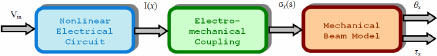
The actuation of the IPMC has been modeled in three stages, mimicking the real physical mechanisms which cause the actuation (see Figure 2.4). A lumped parameter nonlinear electric circuit is used to predict the current absorbed by the polymer and resulting ion flux through the polymer, which is the major mechanism for actuation [SHA 01b, BON 07]. The current flow through the polymer is coupled to the ion/water flux through the electromechanical coupling term, a linear transfer function, to predict the stress induced along the polymer, σx, as a function of length. The stress in the polymer and any externally applied force or loads are input to the mechanical beam model which predicts the exact elastic curve of the IPMC and hence the resulting mechanical outputs, θx and τx.
Figure 2.4. Schematic diagram of electromechanical IPMC model [MCD 10b]
The IPMC is modeled in cantilever configuration, with one end clamped in copper electrodes (see Figure 2.5(a)). The IPMC model is split geometrically in two parts, as shown below in Figure 2.5(b), to represent the section “clamped” by the electrode and the free “beam” section. Using the electric circuit model the average current flow can be predicted for the two sections, IC and IB. The angular displacement, θT, and the blocked torque, τT, are the mechanical outputs.
Figure 2.5. (a) Cross-section and (b) 3D schematic of IPMC and geometric parameters [MCD 10b]

In order for the model to be completely scalable for different dimensions of the actuator, all parameters throughout the model are expressed in terms of the IPMC geometric quantities. A list of these parameters is given in Table 2.1. All other model parameters will be introduced and their physical representation explained when they are defined in the following text.
Table 2.1. Geometric model parameters
| LT | Total length of IPMC |
| LC | Length of IPMC clamped in electrodes |
| LB | Length of the free “beam” section |
| w | Width of IPMC |
| t | Thickness of IPMC |
| θT | Tip angle |
| τT | Tip torque |
2.2.1. Nonlinear electric circuit
It has been widely reported that the main mechanism for mechanical actuation of an IPMC is the ion and hence water flux through the polymer. It is therefore important to model the current flow in the IPMC as this can be coupled to the ion flow. Also the ability to accurately predict power consumption will be useful for designers.
Due to the characteristics of the material, resistance, capacitance, etc., the current draw is modeled using an equivalent electric circuit. The electrical response is characterized by a dynamic and steady-state response. The steady-state response is a nonlinear function of the input voltage. The dynamic response can be accurately characterized by two resistor-capacitor (RC) networks. It is evident that this capacitive dynamic response gives rise to the back relaxation phenomena as well as hysteresis in the polymer, so the circuit is capable of accurately modeling all these behaviors.
The proposed nonlinear electric circuit is shown in Figure 2.6. Researchers have proposed models using a similar approach previously [NEW 02, BON 07], also models including a nonlinear capacitance of the IPMC have been presented in [POR 08, CUE 09], but this circuit presents a number of advances over these existing models.
Figure 2.6. Nonlinear electric circuit model [MCD 10b]

Variable resistors, RssC and RssB are used to model the nonlinear steady-state absorbed current in the clamped and beam section respectively. The RC branches 1 and 2 represent the dynamic response of the polymer through the clamped section, while branches 3 and 4 represent the dynamic response through the free section of the IPMC. The two shunt resistors Re/2 represent the electrode surface resistance and are the average of the ohmic resistance of the surface of the IPMC electrodes. VB is the average voltage through the polymer thickness in the free beam section, that is after half the ohmic loss along the electrodes. The electrode resistance Re has been measured experimentally using a four-point probe technique, and then the RS or sheet resistance value can be calculated in “ohm/square”. Re can then be expressed in terms of the geometry of the IPMC only and hence can be scaled for different sized actuators using equation [2.1].
RssC and RssB account for the nonlinear phenomenon which occurs in the IPMC at very low frequencies and steady-state. They also incorporate the equivalent “through-resistance” of the hydrated polymer membrane. These two material properties cannot be directly experimentally measured and so are consequently combined and expressed as an equivalent resistivity, ρSS. The resistivity, which is dependent on the input voltage, is found empirically through the steady-state relationship between absorbed current and input voltage to be approximated as the third-order polynomial in equation [2.2], whose independent variable is input voltage.
The values for RssC and RssB can be calculated using circuit analysis at steady-state. The resistances are then converted to an equivalent resistivity, ρSS, using equations [2.3] and [2.4] and then can be scaled to any IPMC dimensions.
R1, R2, R3, and R4 represent the resistance against charges flowing through the IPMC that are involved in the dynamic response. They are expressed in terms of the IPMC geometry and an equivalent resistivity in order to enable them to be scaled for different sized actuators. The portion of IPMC in the clamped and free sections have the same material properties and therefore are represented with matching resistivities ρf and ρs as in equations [2.5]–[2.8], where ρf represents the resistance against fast flowing charges and ρs represents the resistance against the slow flowing charges through the polymer material.
Similarly, capacitors C1, C2, C3, and C4 govern the time constants for the charges flowing through the IPMC that are involved in the dynamic response. They are expressed in terms of the IPMC geometry and an equivalent permittivity in order to enable them to be scaled. The portions of IPMC in the clamped and free sections have the same material properties and therefore are represented with matching permittivities εf and εs as in equations [2.9]–[2.12], where εf controls the time constant for the fast flowing charges and εs controls the time constant for the slow flowing charges through the polymer material.
Now that all the parameters for the electric circuit have been defined, the circuit can be analyzed and the current absorbed by the IPMC predicted.
2.2.2. Electromechanical coupling
It is widely accepted that the conversion of electrical energy to mechanical energy is due to the inner charge/water molecule redistribution [SHA 01b, BUF 08]. A number of microscopic actuation mechanisms give rise to the macroscopic deformations of the IPMC [BUF 08]. This is an extremely complex and also stochastic process, which is still not fully understood, so will introduce far too much complexity to the model. To ensure the model is practical yet still realistic, an assumption is made that the electric current flow at any point along the length of the beam can be linearly coupled to the ion/water flow and hence to a longitudinal induced stress of the IPMC beam at that point. This is physically interpreted as the amount of mass of water that flows through the thickness of the beam is directly proportional to the amount of swelling and stress in one side of the IPMC.
A number of different forms for the linear electromechanical coupling transfer function CEM(s) were considered and tested. Based on these tests and work in [BON 07] by Bonomo et al., the most accurate response was achieved with the form shown below, equation [2.13], which includes one zero and two poles.
The values K, Z, P1, and P2 are found empirically. The stress as a function of length along the IPMC can then be calculated by:
2.2.3. Mechanical beam model
The stress generated along the length of the IPMC, as a result of a voltage input, can be converted to a bending moment or electrically induced moment (EIM), using the “flexure formula”, ![]() where y is the direction, from the neutral x axis in the y direction and I is the moment of inertia about the neutral axis. It has been reported in literature that the electromechanical conversions occur at the interface between the electrode and the polymer membrane [NEM 00, NEW 02], using this fact, y is taken as t/2.
where y is the direction, from the neutral x axis in the y direction and I is the moment of inertia about the neutral axis. It has been reported in literature that the electromechanical conversions occur at the interface between the electrode and the polymer membrane [NEM 00, NEW 02], using this fact, y is taken as t/2.
Now the EIM can be calculated as a function of length in the Laplace domain ![]() .
.
The EIM and all other moments which are induced in the IPMC beam as a result of externally applied forces or loads are added to calculate the resultant total bending moment. In this way the proposed model can accommodate any external force/moment or load that acts anywhere along the length of the IPMC. This makes the model extremely useful in mechanical design.
In order to relate bending moment to the beam deflection commonly the approximation M / EI = d2v / dx2 is used by assuming a shallow curve where EI is the product of the modulus of elasticity and moment of inertia of the IPMC. When modeling the IPMC with large inputs, this assumption will not hold true, and therefore will not give an accurate representation of the true displacement of the beam. Also using this method, as has been done in previous models [NEW 02, BON 07, CHE 08], will only give a linear displacement as a function of the length and not the actual elastic curve and bending displacement. This IPMC model needs to be accurate for large displacements. Therefore to overcome this issue, the beam has been “segmented” into smaller pieces along its length. Providing the segments are small enough, they can be analyzed individually and the shallow curve assumption will hold true. Each segment will have its own elastic curve and when put together will make up the entire elastic curve of the IPMC beam. Using this method will then allow the true shape of the bending actuator to be found, an angular displacement and not a simple linear approximation as in previous models [NEW 02, BON 07, CHE 08]. An example of a segmented curve is shown in Figure 2.7(a), with a segment length of 1 mm and the combined resulting curve for the IPMC with 30 mm free length is shown in Figure 2.7(b). The individual segment displacements are more than an order of magnitude smaller than the length of segment, which ensures that the shallow curve assumption holds true.
Figure 2.7. Typical deflections for an IPMC with 30 mm free section and segment length of 1 mm (a) individual segments, (b) combined elastic curve for IPMC [MCD 10b]
2.2.4. Parameter identification and results
All the model parameters were identified using a Nafion®-based IPMC actuator 24 mm long, 10 mm wide, and an average thickness of 0.7 mm, with Pt-coated electrodes (see Table 2.2), using solely the blocked force results. The agreement between the simulated and experimental free displacement and force at varying displacements then verifies that the model is accurate for the full actuation response of the IPMC.
Table 2.2. Identified model parameters
| RS | 21.12 Ω |
| a | 8.84×10⁻⁴ |
| ρS | –4.3983|Vin| + 15.446 |
| ρf | –1.2561|Vin| + 4.4083 |
| εS | 0.4420|Vin| + 0.3993 |
| εf | 0.1981|Vin| + 0.5078 |
| K | –9,434.0|Vin| + 74,869 |
| Z | 0.1431|Vin| + 4.3595 |
| P1 | 2.8180|Vin| + 7.7198 |
| P2 | –0.0321|Vin| + 0.4499 |
| E | 0.1757 GPa |
| I | 0.2858×10⁻¹² m4 |
The model with the parameters identified as in Table 2.2 is simulated for 60 seconds and both absorbed current and blocked force are compared with actual measured values to evaluate their correlation. Figures 2.8(a)–(c) plot the simulated and actual experimental results for the current draw for the actuator at 1 V, 2 V, and 3 V respectively. The plots clearly show the excellent correlation between the simulated current draw and the actual measured current draw. It can be seen that the peak current draw, the dynamic decay, and the steady-state values can all be accurately predicted by the model.
Figure 2.8. Experimental and simulated current for (a) 1 V, (b) 2 V and (c) 3 V step inputs [MCD 10b]

Figure 2.9(a) plots the corresponding simulated and actual measured blocked force for 1–3 V inputs at zero displacement. Again it can be seen that there is a good agreement between the simulated and experimental results. The 2 V experiment is lower than the simulated, but with the unrepeatable nature of the IPMC, some deviations can be expected and are acceptable. The results of the free deflection experiments and corresponding model simulation are shown, see Figure 2.9(b) for 1–3 V. The results show a good match to the actual measured displacements.
It can be seen that the model captures both the nonlinear steady-state characteristics, after the system has been left for a long time to settle, as well as the fast dynamic response of the IPMC at a large range of voltage inputs (up to 3 V). The model also correctly predicts the back relaxation phenomena to a DC input.
The equivalent electric circuit has also been designed to accurately account for the hysteresis effects exhibited by IPMCs [ZHE 05, PUN 07, SHA 07]. The model is simulated with a 3 V amplitude sinusoid wave of 0.2, 0.1, and 0.025 Hz, over 60 seconds. The results are shown in Figure 2.10. It can be seen that there is an obvious hysteresis loop as the current draw and tip displacement follow a different path when the voltage is increasing to when the voltage is decreasing. The hysteresis loop predicted by the model is caused by the transient behavior of the variable RC branches in the electrical model. The level of hysteresis is therefore dependent on the input voltage and frequency. This is shown in Figure 2.10 by the different paths followed for the different frequencies simulated, which is also observed in the real system. It is also clear that the simulated data indeed captures the nonlinearity.
Figure 2.9. Experimental and simulated (a) blocked force, (b) displacement for 1, 2, and 3 V step inputs [MCD 10b]
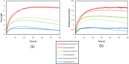
Figure 2.10. Simulated (a) current draw and (b) tip displacement vs. input voltage for a ±3 V sinusoid wave input of 0.2, 0.1, and 0.025 Hz over 60 seconds [MCD 10b]

The model is also capable of predicting the relationship between the force and displacement. The blocked force has been measured at a number of different displacements. Figure 2.11 shows the experimental passive blocked force (0 V input) at varying displacements and the peak blocked force for –3 V to +3 V inputs at each displacement. The model is then simulated for the same conditions. The results plotted show the close agreement between the model and the actual measurements. This demonstrates the model’s ability to predict the force as a function of displacement as well as the free displacement and velocities of the IPMC, showing that the model is indeed accurate for the complete actuation response of the IPMC.
Figure 2.11. Experimental and simulated peak blocked force at varying tip displacements for -3 V to +3 V step inputs [MCD 10b]

All parameters have been developed with a physical interpretation and are expressed in terms of IPMC geometry to ensure scalability. Experiments were carried out using two different samples based on the same Nafion®-Pt material, one 30 × 10 × 0.7 mm and another 35 × 10 × 0.7 mm actuator, both with a 5 mm clamped section. Figure 2.12 compares the results of the experimental data and the model predictions for the 30 mm and 35 mm long actuators.
These plots clearly show that the complete actuation response, force, and displacement, in both the dynamic and steady-state range, of an IPMC actuator can be determined for different actuator geometries. Although there are some small deviations, it can be seen here that both the dynamic and steady-state response can be reasonably accurately simulated for force and displacement, with 1, 2, and 3 Vs.
A complete model for the actuation response has been developed which is a useful tool used to design mechatronics systems for a real life applications. In the remainder of this chapter examples are given to demonstrate how the model is used to design a stepper motor and a robotic rotary joint.
Figure 2.12. Experimental and simulated (a) blocked force and (b) displacement of a 30 mm long IPMC, and (c) blocked force and (d) displacement of a 35 mm long IPMC [MCD 10b]

2.3. IPMC stepper motor
A stepper motor has been developed which can operate in air and works by converting the bending actuation of IPMCs into a rotational motion of the motor. The motor is designed with a view to miniaturization and use in micro-robotics where the force output requirements are low, but other advantages of IPMCs are important, such as weight and power availability for remote and embedded systems.
The development of this novel stepper motor demonstrates an innovative mechatronics design process for a complete system with integrated IPMC actuators. The motor has been developed by utilizing the novel model for IPMC actuators incorporated with a complete mechanical model of the motor. The entire system is simulated, and an appropriate size IPMC strip chosen to achieve the required motor specifications and its performance verified. The system has been built and the experimental results are validated to show that the motor works as simulated and can indeed achieve continuous 360° rotation, similar to conventional motors.
2.3.1. Mechanical design
The conventional stepper motor is a brushless, synchronous electric motor which divides a full rotation of the motor into a number of “steps”. A stepper motor configuration shown in Figure 2.13 was chosen for achieving rotary motion using IPMCs for a number of reasons, including simple design and working mechanism to convert IPMC bending to rotary motion, very low contact area between IPMC and device resulting in low friction, and also the ability to use open loop control architecture. Advantages of the IPMC stepper motor in comparison to a traditional stepper motor include low cost, lightweight design and low power consumption.
The IPMC stepper motor works by sending a voltage sequence to the IPMC actuators which will cause them to bend into contact with the pins attached to the motor shaft; this applies a force to the motor which will then result in controlled rotary “stepping” motion. The pins are placed on the top and bottom layer, each corresponding to one IPMC. The pins on each layer have 90° separation from each other and the top pins are 45° out of phase from the bottom pins. The stand is adjustable for accommodating different size IPMC strips as required. A pulsed input voltage of ±3 V is used to actuate the motor, with each pulse or step corresponding to a 45° rotation.
Figure 2.13. CAD model of the proposed stepper motor [MCD 10a]

2.3.2. Model integration and simulation
The stepper motor has been designed using CAD tools and mathematical analysis and is integrated with the developed IPMC actuator model. The motor friction is added to the system model, using a standard Coulomb and viscous friction model, to make a realistic simulation and see if the IPMC can actually move the motor shaft. The motor friction force was found experimentally to be 0.27 gf for static and 0.21 gf for dynamic motion. Using these forces the friction coefficients were calculated and inputs obtained to create an entire system model which can accurately represent the real life situation.
Different lengths of IPMC were simulated and the length of 35 mm long (clamped length 5 mm) and 10 mm wide was found to give the desired performance, both force and deflection, that was required to actuate the motor. Designing the system in simulation has first allowed the system to be extensively tested and the performance verified before the prototype was built. This demonstrates the usefulness of the developed model for designing IPMC-actuated mechanisms. The simulated performance of the system is shown in Figure 2.14. It can be seen that there is a pause in the operation of the motor between steps. This is necessary in the design with two IPMCs to avoid the motor pins clashing with the IPMC that is returning to its home position.
2.3.3. Experimental validation
The actual stepper motor is rapid prototyped, shown in Figure 2.15, and experiments are undertaken to test the actual performance and verify all the simulations. Figure 2.16 shows the actual measured tip displacements of the IPMCs when they are being actuated in order to move the motor. They are measured using 2 Banner LG10A65PU laser sensors with a 3 µm resolution.
There is a reasonable correspondence between the simulated motor and the actual experimental results. It can be seen that at the beginning the IPMC has a larger displacement and it starts to degrade in performance. This is mainly due to the fact that the motor is operating in air for a period of time and the IPMCs exhibit highly time-varying behavior in this type of environment. Despite this the motor does act as the simulation predicts and rotary motion is achieved. The camera shots in Figure 2.17 show the motor in operation, and again it can be seen that the system does operate as predicted.
Figure 2.14. Simulated input voltage and displacement for (a) IPMC 1 and (b) IPMC 2 and (c) resulting motor shaft displacement [MCD 10a]

Figure 2.15. Rapid prototyped stepper motor

Figure 2.16. Laser displacement of the IPMCs driving the stepper motor [MCD 10a]

Figure 2.17. Camera shots of motor in operation (a) at initial position, (b) after step 1, after step 3, (d) after step 5, (e) after step 7, (f) 315° rotation completed and IPMCs back to home position (Note: the black dot) [MCD 10a]

2.3.4. Extension to four IPMCs
It has been demonstrated that the stepper motor works as simulated and therefore it is valid to believe that this model and simulation technique can be extended to other devices. The next step to improving the performance of the stepper motor is to remove the pause in the operation to achieve continuous rotation as with traditional rotary motors.
A new design incorporating four IPMCs and using the same principle as the previous design has been proposed. The IPMCs work in two pairs, with each pair acting similarly to the two IPMCs in the previous design. In simulation it is shown that the two pairs must be 90° or more out of phase from each other to avoid the IPMC clashing when returning to the home position. The phase also has to be a multiple of 45° to remove the pause and achieve constant motion. It has therefore been designed that the IPMC pairs are 135° out of phase. The simulation results are shown in Figure 2.18 and prove that this will remove the pause in the system and that the new design can indeed achieve continuous motion.
Figure 2.18. Motor shaft angular displacement for a four IPMC stepper motor [MCD 10a]

The time step can be altered to speed up the motor, but there is a limit to the step time as the IPMCs still need to have enough time to reach their home positions. A smaller voltage could also be applied, but this would decrease the available torque output of the motor and may decrease the speed of the motor as well. Variations on the design can easily be simulated using the model to verify their design before going on to build the system.
2.4. Robotic rotary joint
A variety of literature has been produced on free-bending of IPMC actuators, but little research has been carried out on using them to drive mechanisms. This application explores the potential for applying IPMC to driving miniature rotary mechanisms, for small-force robotic manipulators, or positioning systems. Rotary joints are commonly found in robotics, industrial applications, biology, and many other areas.
The motivation is to develop a system that can be used in a much wider range of applications that would benefit from lightweight, flexible actuators driving mechanisms such as linkages and rotary joints, which account for a sizeable portion of modern technology. Furthermore, real life issues such as mechanism dynamics, friction, and weight need to be tackled so these actuators could potentially be used as replacements for existing, more bulky devices.
2.4.1. Mechanical design
A simple lightweight, rigid, single degree-of-freedom rotary joint has been designed which incorporates an IPMC in the commonly used cantilevered configuration, as shown in Figure 2.19. The rotary linkage has a length of 30.1 mm, a width of 20.0 mm wide, and total weight of 1.1 g. At the end of the rotary linkage is a slot compartment. The IPMC pushes against the side walls of the slot when actuated to move the rotary linkage. When assembled, the rotary linkage can be driven up to 40° in each direction which exceeds the capabilities of the IPMC actuators based on the results of the open loop deflection experiments. Results from 20 consecutive friction tests revealed that the average blocking force of the rotary mechanism is 0.084 gf with a standard deviation of 9.725 × 10⁻⁵ gf.
Figure 2.19. Photo of the rotary mechanism (a) without IPMC and (b) actuated by an IPMC with –4 V step voltage
2.4.2. Control system
In order to harness the wide-ranging advantages of IPMC actuators and to aid their successful implementation into real systems, the actuation response of an IPMC must be effectively controlled. However, this is not a trivial task due to their complex behavior. Open loop control has been successfully implemented for the stepper motor but more advanced closed loop control will be needed for the rotary joint.
In order to effectively control the system displacement a one degree-of-freedom proportional integral derivative (PID) control architecture is implemented, as shown in Figure 2.20. It has been demonstrated in [RIC 03, YUN 06b, FAN 07, MCD 10c] that simple linear PID control can in fact accurately control the IPMC system over a certain operating range.
Figure 2.20. One degree-of-freedom PID closed loop control system

2.4.3. System parameter tuning
Most IPMC controllers that have been realized are tuned in simulation using an approximate plant model. The performance is then assessed, also in simulation, before implementing the controller on the real system. One major issue with this method is the development of a suitably accurate IPMC model which is complex and time consuming as the IPMC is extremely nonlinear, time-variant, and environmentally sensitive. In addition the controller must be further fine-tuned on the real system to account for variability between the model and the real plant. The controller is also sample specific so it cannot be transferred to a different IPMC actuator. Consequently it is highly desirable to develop an automatic tuning method.
Iterative feedback tuning (IFT) is an automatic tuning method which seeks to optimize the controller parameters in the system. The IFT algorithm applied to this application enables the IPMC to be adaptively tuned without the need of any model or knowledge of the system. We simply set the IPMC and then run the tuning algorithm to obtain an optimally tuned system. This controller tuning method eliminates the need for an accurate model in order to accurately control the IPMC actuator. This is a completely new way of thinking for smart materials as up until now research emphasis has been on the modeling of materials in order to be able to control their behavior. This new model-free approach to controller design presents a major step forward for IPMC technology, toward wide acceptance as a viable alternative to traditional actuators.
Even though some model-based control methods have shown reasonable performance they have only been proven to operate well only over a short period of time. The fact is that IPMC dynamics do vary far from their initial state and the performance of a static model-based controller can become unacceptable. If the system dynamics of an IPMC drift far from the developed model then the effort spent on modelling the system becomes redundant. The system dynamics can change so much that they will even shift outside the acceptable range of a robust control design. The IFT algorithm overcomes these issues as it will adaptively tune toward an optimal state whatever the system dynamics change to.
It has been decided that since a model has been previously developed for the design and development of mechanical systems then it will be useful to design a model-based controller for comparison between the performance of the IFT algorithm and a model-based design, demonstrating IFT’s adaptive ability in comparison with a non-adaptive model-based control system. The model-based controller can also be used as a starting point for the IFT, in this way the IFT algorithm will take over the model-based approach and automatically tune the system toward an optimal state as the system dynamics change.
2.4.3.1. IFT overview
IFT is an automatic tuning method that iteratively optimizes the controller parameters, which are used to regulate the performance of an unknown plant [HJA 94]. This tuning method uses the response of the actual system to determine new updated and improved control parameters in order to minimize some cost function of the system, in this case a least squares fit of the tracking error. As the controller parameter updates are based on only experimental data from the actual system, there is no need for any knowledge or model of the system. The implementation of IFT has shown good results in both laboratory and industrial applications such as control of profile cutting machines [GRA 07], speed and position control of servo drive [KIS 09], temperature regulation in a distillation column [HJA 98], and control of photo resistant film thickness [TAY 06]. The method has traditionally been used to tune systems off-line, or before they commence standard operation due to the fact that a “special” gradient experiment, whose trajectory may deviate far from the trajectory of the normal experiment, is needed to calculate the updated parameters. A full description of the IFT algorithm can be found in [HJA 98] and a concise explanation of the key details for implementation is presented in the following section.
2.4.3.2. Algorithm for IFT implementation
The control system presented in Figure 2.20 will be tuned using the IFT algorithm to successfully control the IPMC system. IFT is a time domain approach whose objective is to minimize a cost function or design criterion based on the controller performance in order to obtain an optimally tuned system. There are a number of different design criteria which have been proposed in the literature based on tracking error and control effort. The design criteria that will be used for the rotary joint controller is a quadratic function based on a least squares fit of the tracking error, ![]() , as shown below in equation [2.15].
, as shown below in equation [2.15].
where ρ is a vector of the controller parameters to be tuned, N is the total number of time steps for a given experiment and ![]() is the system error at discrete time step t. The premise of the IFT algorithm is to find a minimum of the design criteria, J, in this case finding the minimum tracking error over the entire experiment. In order to locate the minimum of the criteria the gradient is found by differentiating equation [2.15] and finding the solution to make this equal to 0, equation [2.16].
is the system error at discrete time step t. The premise of the IFT algorithm is to find a minimum of the design criteria, J, in this case finding the minimum tracking error over the entire experiment. In order to locate the minimum of the criteria the gradient is found by differentiating equation [2.15] and finding the solution to make this equal to 0, equation [2.16].
Applying the iterative algorithm in equation [2.17], the solution for ρ can be found to obtain the minimum error for the system. This is a gradient search algorithm:
where Ri is an appropriate positive definite matrix which determines the search direction for the optimization, i is the iteration number and γ is a positive real scalar which controls the step size. Using the identity matrix for Ri gives a negative gradient direction. It is commonly accepted in the literature [HJA 98, HJA 02, GRA 07] that using the Gauss-Newton approximation of the Hessian of J(ρ) for Ri gives improved results. This becomes more important when the sample size is small. The Hessian is given below in equation [2.18].
In order to solve for the updated controller, two signals are needed, ![]() , and
, and ![]() for equation [2.16]. These must be found independently such that they are unbiased by each other [HJA 02]. In the standard IFT algorithm these signals are found over two independent experiments as follows:
for equation [2.16]. These must be found independently such that they are unbiased by each other [HJA 02]. In the standard IFT algorithm these signals are found over two independent experiments as follows:
1. A first experiment is conducted under normal operating conditions with an external deterministic reference signal, r, applied at the input, and the output y is recorded. ![]() can then be found from
can then be found from ![]() .
.
2. A second, “special” experiment is then conducted in order to calculate the gradient, ∂yt (ρ)/∂ρ. This is the same as the first experiment, except the input, r, is the error ![]() from the first experiment.
from the first experiment.
With these two batches of data ![]() is the error from the first experiment and ∂yt (ρ)/∂ρ is calculated by the following.
is the error from the first experiment and ∂yt (ρ)/∂ρ is calculated by the following.
For the given control system used for tuning the IPMC, Figure 2.20, the closed loop output is defined as:
Then by differentiating the output, ∂yt (ρ)/∂ρ can be found as:
By comparing the term in the square brackets in equation [2.20] and equation [2.19] it can be seen that the term in the square brackets is the result of injecting the error from the first experiment through the closed loop system. The output from the plant for this second experiment gives the term in the square brackets in equation [2.20]. The two terms ![]() can be found by differentiating the controller itself and hence
can be found by differentiating the controller itself and hence ![]() can be established. Using this result, the Hessian can be calculated from equation [2.18] and also
can be established. Using this result, the Hessian can be calculated from equation [2.18] and also ![]() can be found leading to the new updated controller parameters, ρi+1, which will give an improved controller for the system. This procedure is then repeated for the desired number of iterations, or until the desired system performance is achieved.
can be found leading to the new updated controller parameters, ρi+1, which will give an improved controller for the system. This procedure is then repeated for the desired number of iterations, or until the desired system performance is achieved.
2.4.4. Experimental tuning results
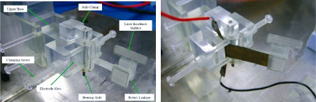
Experiments were undertaken using a custom test rig which supports 2 copper clamps which act as electrodes to pass the voltage to the IPMC. The IPMC and clamps are placed in a container of de-ionized water in order to avoid rapid dehydration and potential damage to the IPMC. This will also slow the time-varying behavior so the performance of the tuning algorithm can be more objectively assessed. Testing was undertaken based on the free deflection of the IPMC to prove the control system required for the robotic joint.
A Nafion®-based IPMC was used, with Pt electrodes. The IPMC was 35 mm long, 10 mm wide with a thickness of 200 µm. The clamped length was 5 mm. This relatively long length of IPMC was chosen because most research has been carried out with shorter lengths of IPMC as actuation response is more linear with shorter IPMCs [ANT 08, HUN 08]. This research is attempting to tackle the nonlinearity so therefore a long length was used. Also shorter IPMCs cannot achieve large displacements so a long length will be needed to ensure that both micro (<1 mm) and macro (>1 mm) displacements can be investigated. With the specific IPMC used for this research, up to a 3 mm displacement will be input as the target reference.
Due to the desired applications in robotics and biomimetics, the control system was designed to be accurate for changes in set point, in terms of both the transient and steady-state response. In order to tune for this, the reference trajectory was a stair-step function to the desired set point to be tuned. The experiments will be 60 s long with a reference of: positive target displacement for the first 15 s, then step back to zero displacement until 30 s, then negative target displacement until 45 s, and finally to zero displacement until 60 s. This reference will ensure that the IPMC has been tuned in both directions, as it has been shown that due to imperfect fabrication techniques the IPMC can have different performance in different directions. This reference will give tuning for four transient periods as well as steady-state behavior.
The initial controller parameters, Kp, Ki, and Kd, were chosen by tuning the IPMC through model simulations. This will give the benchmark model-based control system for performance comparison. The derivative gain in a PID controller contributes based on the change in error, and therefore will amplify any high frequency noise that may be present in the laser sensor or control electronics. It was desired to control the IPMC to micron displacements, where the noise starts to become an appreciable part of the feedback signal, so a high Kd value is likely to introduce large high frequency oscillation and possibly make the system unstable. Also it has been shown by Liu in 2010 [LUI 10] that PI controllers can exhibit good response in controlling IPMCs. For these reasons the authors were confident to start with a PI controller by setting the derivative gain to 0 and letting the IFT tuning algorithm decide how much derivative action to include. The chosen initial model-based values were Kp = 1,000, Ki = 500, and Kd = 0.
In order to ensure convergence to the local minimum of the design criteria the data set has been chosen large, 600 samples (60 s at 10 Hz), and the step size for the control parameters must be chosen relatively small. The step size must be small enough to ensure the controller does not “jump too far” and result in an unstable system, but be large enough so that there is a rapid convergence to the minimum design criteria, otherwise too many iterations will be needed, making the algorithm impractical.
The step sizes chosen for the IPMC system were γKp = 1, γKi = 1, and γKd = 0.5. As a rule for the IPMC system the step size was chosen so that control parameters would update by no more than 100% of the previous value. From the experiments undertaken it has been shown that this step size will ensure that the system will remain stable, but also achieve a rapid convergence within five iterations. The value for step size of the derivative gain was chosen as half of that for the proportional and integral gain because for a large increase in derivative term it is possible the system may iterate to an unstable system at low deflections in the presence of large noise input.
With the setup completed, the IFT algorithm was run on the IPMC using the initial controller values and step sizes. The IFT algorithm was run to tune the IPMC controller for displacements in the micro- and macro-range, reference signals ranging from 100 µm to 3 mm. This was done as due to the nonlinear nature and varying dynamics of the IPMC at varying displacements it is expected that the optimal controller parameters would vary considerably depending on the target displacement.
The time response for the 3 mm target displacement is shown in Figure 2.21. First the initial output using the model-based PI controller is shown (see Figure 2.21(a), then the performance of the system with the next five consecutive iterations of the controller parameters, found by the automatic IFT algorithm, are shown (see Figures 2.21 (b)–(f) respectively).
It is clear to see that the initial controller had large oscillation in the first quarter, large overshoot starting at 30 s, and also some overshoot and oscillation when finally returning to zero displacement. Even after just one iteration of the control parameters there was an obvious improvement in the response, with the oscillations in the first 15 s reduced significantly as well as the overshoot at 30 s. After each iteration the controller parameters were updated and it can be seen from the time response that the IPMC output drastically improved. After five iterations the performance of the controller for a 3 mm displacement had significantly improved. The improvement can be quantified as a 56% of the design criteria J(ρ).
Figure 2.21. Time response over five iterations of the controller for 3 mm step displacement [MCD 10c]

This same procedure was undertaken for 100 µm, 200 µm, 300 µm, 500 µm, 1 mm, 1.5 mm, 2 mm, 2.5 mm, and 3 mm displacements. It was found that at 100 µm and 200 µm, despite being able to track accurately to the target displacements, the noise level from the sensor and electronics was too large to accurately tune for these displacements. The tuned parameters were very inconsistent because of the low signal-to-noise ratio (SNR). This was confirmed by the fact that the IFT algorithm kept the proportional gain at these displacements at zero or very low to ensure that noise was not amplified.
The full set of results for the final tuned values for each displacement is given in Table 2.3, along with the percentage improvement of the controller design criterion. The major success of the IFT algorithm in tuning the system from the initial model-based controller is very clearly seen.

2.4.5. Gain schedule nonlinear controller
In order to achieve accurate control over a large range of target displacements, on the micro- and macro-scale, a gain scheduled (GS) nonlinear control architecture is developed to extend the PID control system. This allows the control parameters to adapt depending on the states of the system. This is necessary as it can be seen that the optimal controller gains do vary significantly based on the reference input. This GS controller has the ability to automatically adapt itself in order to tackle the nonlinearities and time-variance to achieve accurate positioning over a large displacement range.
The schedule for the controller gains has been chosen based on a function of the reference trajectory, that is the gains vary depending on the target displacement of the joint. Its architecture is shown in Figure 2.22 and the task now is to find the function fGS(r) for the controller.
Figure 2.22. Block diagram of proposed GS controller
The PID controller has been tuned using IFT for a range of different target values, resulting in a set of tuned linear controllers for different reference trajectories. Now in order to turn the finite linear controllers into a continuous controller, the control parameters must be interpolated in order to schedule the gain continuously over the operating range. The tuned controller gains Kp, Ki, and Kd are plotted in Figure 2.23 as a function of target displacement. There is a clear trend in the relationship with the control parameters and target displacements. After some analysis it was found that a logarithmic fit would give the best correlation between these parameters. These trends for the control parameters are plotted on the graph in Figure 2.23 and the relationships are presented in equations [2.21]–[2.23].
Figure 2.23. Final controller parameters after IFT at varying displacements [MCD 10c]

The controller was also tuned for references of 100 µm and 200 µm, but because of the low SNR the tuned parameters were very inconsistent. The tuned values for Kp and Ki at 100 µm and 200 µm were in the region of those obtained for 300 µm and the values for Kd were slightly lower than that for 300 µm at these small targets. For this reason it was decided to restrict the controller parameters at their 300 µm values, that is if the target displacement was less than 300 µm then use the values scheduled for 300 µm. This is also necessary to prevent Kp and Ki from increasing extremely high because their schedule approaches the zero reference asymptotically.
An interesting observation is that if the IPMC was linear, then the controller gains would be constant across all target displacements. This in itself validates that the IFT algorithm has successfully tackled the nonlinear characteristics of the IPMC. It can also be observed that the IFT algorithm realizes that the SNR is low at small displacements and consequently reduces KP accordingly as not to amplify the noise at these levels.
Now the schedule to change the gains, fGS (r), has been developed, the nonlinear GS controller is complete and ready for implementation.
2.4.6. Gain schedule vs. PID controller
The developed nonlinear GS controller was tested and its performance compared to a conventional PID controller with the IFT-tuned parameters for 1.5 mm displacement, as this is in the middle of the range of IPMC operation. The design criteria for IFT, equation [2.15], was used as a quantitative measure of the performance of the controllers and qualitative measures such as overshoot and settling time are also analyzed.
In order to test the performance of the GS controller versus the conventional PID controller for changes in set point, which is what the controller is designed for, a random stair-step sequence of varying amplitude was used as input. Both the micro and macro targets were used. The results of this test are shown in Figure 2.24. By examining the plot it can be seen that the GS controller had a much smaller overshoot at all of the set point changes, except for at micro targets (30 s and 90 s). This is due to the fact that the proportional gain is high when the target displacement is low as seen in Figure 2.23. This suggests that the cut-off region in the schedule, which was set at 300 µm, may be too low. Using a higher cut-off (say 500 µm) will restrict the Kp and Ki values at micro displacements and the GS controller may not over shoot as much.
The settling time after a set point change is better for the GS controller in all cases, even at the micro targets (30 s and 90 s), where there is more overshoot. Comparing the overall error for the controllers using the design criteria the GS controller is 17% better.

Figure 2.24. Random stair-step reference input for comparison of control performance [MCD 10c]

In order to demonstrate the versatility of the GS controller to other input signals, sinusoid reference trajectories were tested versus the conventional PID controller. This will result in dynamically varying control parameters as the reference signal is continuously changing. A number of experiments were undertaken to assess the performance under different conditions inside the desired operating range of the IPMC.
Figure 2.25(a) shows the 33 × 10–3 Hz signal with a micro amplitude of 500 µm. It can be seen that both controllers follow the reference very well, despite a relatively high level of noise. By inspection, the performance of both controllers are comparable, but using the design criteria it can be seen that the GS controller does perform slightly better, J(PID) = 1.32e–9 and J(GS) = 1.15e–9.
Figure 2.25(b) shows the 33 × 10–3 Hz signal with a large amplitude of 3 mm. Both controllers track the reference extremely well and again by inspection the performance of both controllers are again comparable. Using the design criteria, J(PID) = 6.55e–9 and J(GS) = 5.35e–9, so again the GS controller does perform better.
It has been shown that the designed controllers can accurately track a dynamic reference with a time period of 30 s, so a faster signal of 0.1 Hz was tested. Figure 2.26(a) shows the 0.1 Hz performance at a 500 µm amplitude for the two controllers. It can be seen that the standard PID controller has a considerable level of overshoot and then consequently lags the reference signal. It is clear that the GS controller is performing better and this is confirmed by the design criteria, J(PID) = 16.3e–9 and J(GS) = 2.35e–9.
Figure 2.26(b) shows the performance with a reference amplitude of 3 mm at 0.1 Hz. Similar to the 500 µm reference it is clear to see that the standard PID controller exhibits overshoot. This high level of overshoot again results in an output lag. By inspection the GS controller performs a great deal better and this can be confirmed by the design criteria, J(PID) = 13.6e–8 and J(GS) = 6.96e–8.
Figure 2.25. 33 × 10–3 Hz sinusoid inputs for (a) 500 µm and (b) 3 mm amplitude [MCD 10c]

Figure 2.26. 0.1 Hz sinusoid inputs for (a) 500 μm and (b) 3 mm amplitude [MCD 10c]

2.5. Discussions
Although modeling the IPMC has been a large research focus for 15 years there is still no complete and widely accepted model that has been developed to predict the mechanical output and even the underlying mechanisms for actuation are not fully understood. This is partly due to the very complex nonlinear, time-varying, and environmentally sensitive nature of the composite material [YAG 04, BON 07, BUF 08]. The development of a suitable IPMC model which will accurately represent the real system is extremely complex and time consuming. The model presented acts as a very useful tool for mechanical design and simulation of the mechatronics systems. It however is not accurate enough over time to develop a controller based solely on this or any other model. It has however served as an excellent tool for mechanical design and simulation for the applications presented and has given a good starting point to develop an acceptable stable controller, for the IFT algorithm to tune from.
The IFT algorithm has the major advantage of being model-free which is extremely useful for IPMCs and any other mechatronics systems where a model of the system is not available and developing one maybe too complex. With regard to IPMCs this is a major step forward, as modeling has been a large research focus for 15 years and there is still no widely accepted model for the actuation response. This will have a major impact in this field and will aid in the implementation of IPMCs into real mechatronics systems, which up until now have been restricted due to limitations in modeling and control.
The hysteresis behavior and other nonlinearities are not directly addressed by the IFT controllers, as some model or knowledge of the system would be necessary to account for this [ZHE 08], which is specifically what the IFT algorithm is avoiding. Despite this the controller may well instinctively compensate for some part of the hysteresis as it is automatically tuning online as the system operates in certain modes.
The IFT tuning has a modified experiment every third time period, even in the online case, which can cause some deviation from the desired reference. To minimize the effect of this the tuning experiment may be undertaken say every 10th or even 100th iteration, depending on how quickly the system is varying and how quickly the system needs to converge to an optimal state. For example if a system is operating all day, it may need to be tuned for an hour per day to keep the system operating successfully.
2.6. Concluding remarks
Two mechatronic devices have been developed through a thorough design process. First the IPMC actuator was modeled in order to develop a useful tool for developing and testing the performance of the applications before implementing them in real life. Control systems have been developed and implemented using novel approaches, each tailored to the specific application; i.e. open loop control for the stepper motor, PID, and GS control for the rotary joint mechanism. This has successfully demonstrated the capabilities of IPMCs and the benefits of implementing them as valid alternatives to traditional mechatronic actuators.
2.7. Bibliography
[AHN 10] AHN K.K. et al., “Position control of ionic polymer metal composite actuator using quantitative feedback theory”, Sensors and Actuators A: Physical, vol. 159, 2010, pp. 204–212.
[ANT 08] ANTON M. et al., “A mechanical model of a non-uniform ionomeric polymer metal composite actuator”, Smart Materials and Structures, vol. 17, no. 2, 2008, p. 025004.
[BAR 00a] BAR-COHEN Y. et al., “Challenges to the application of IPMC as actuators of planetary mechanisms”, Proceedings of SPIE — The International Society for Optical Engineering, vol. 3987, 2000, pp. 140–146.
[BAR 00b] BAR-COHEN Y. et al., “Challenges to the transition to the practical application of IPMC as artificial-muscle actuators”, Materials Research Society Symposium — Proceedings, 2000.
[BON 07] BONOMO C. et al., “A nonlinear model for ionic polymer metal composites as actuators”, Smart Materials and Structures, vol. 16, no. 1, 2007, pp. 1–12.
[BUF 08] BUFALO G.D. et al., “A mixture theory framework for modeling the mechanical actuation of ionic polymer metal composites”, Smart Materials and Structures, vol. 17, no. 4, 2008.
[CHE 09] CHEN Z. et al., “A nonlinear, control-oriented model for ionic polymer-metal composite actuators”, Smart Materials and Structures, vol. 18, no. 5, 2009.
[CHE 08] CHEN Z., TAN X., “A control-oriented and physics-based model for ionic polymer-metal composite actuators”, IEEE/ASME Transactions on Mechatronics, vol. 13, no. 5, 2008, pp. 519–529.
[CHE 09] CHEW X.J. et al., “Characterisation of ionic polymer metallic composites as sensors in robotic finger joints”, International Journal of Biomechatronics and Biomedical Robotics, vol. 2, no. 1, 2009, pp. 37–43.
[FAN 07] FANG B.K. et al., “A new approach to develop ionic polymer-metal composites (IPMC) actuator: Fabrication and control for active catheter systems”, Sensors and Actuators A: Physical, vol. 137, no. 2, 2007, pp. 321–329.
[GRA 07] GRAHAM A.E. et al., “Rapid tuning of controllers by IFT for profile cutting machines”, Mechatronics, vol. 17, 2007, pp. 121–128.
[HJA 02] HJALMARSSON H., “Iterative feedback tuning — an overview”, International Journal of Adaptive Control and Signal Processing, vol. 16, no. 5, 2002, pp. 373–395.
[HJA 94] HJALMARSSON H. et al., “A convergent iterative restricted complexity control design scheme”, Proceedings of the 33rd IEEE Conference on Decision and Control, 14–16 December 1994.
[HJA 98] HJALMARSSON H. et al., “Iterative feedback tuning-theory and applications”, IEEE Control Systems, vol. 26, 1998, p. 41.
[HUN 08] HUNT A. et al., “A multilink manipulator with IPMC joints”, Proceedings of SPIE — The International Society for Optical Engineering, 2008.
[KAN 96] KANNO R. et al., “Linear approximate dynamic model of ICPF (ionic conducting polymer gel film) actuator”, Proceedings of Robotics and Automation, IEEE International Conference, 22–28 April 1996.
[KIS 09] KISSLING S. et al., “Application of iterative feedback tuning (IFT) to speed and position control of a servo drive”, Control Engineering Practice, vol. 17, no. 7, 2009, pp. 834–840.
[KOT 08] KOTHERA C.S. et al., “Characterization and modeling of the nonlinear response of ionic polymer actuators”, Journal of Vibration and Control, vol. 14, no. 8, 2008, pp. 1151–1173.
[LAV 05] LAVU B.C. et al., “Adaptive intelligent control of ionic polymer-metal composites”, Smart Materials and Structures, vol. 14, no. 4, 2005, pp. 466–474.
[LUI 10] LIU D., “Design and control of an IPMC actuated single degree-of-freedom rotary joint, mechatronics engineering”, The University of Auckland, New Zealand, 2010.
[MAL 01] MALLAVARAPU K. et al., “Feedback control of the bending response of ionic polymer–metal composite actuators”, Smart Structures and Materials 2001: Electroactive Polymer Actuators and Devices, Newport Beach, CA, USA, SPIE, 2001.
[MCD 09] MCDAID A.J. et al., “A nonlinear scalable model for designing ionic polymer– metal composite actuator systems”, 2nd International Conference on Smart Materials and Nanotechnology in Engineering, WeiHai, China, 2009.
[MCD 10a] MCDAID A.J. et al., “Development of an ionic polymer–metal composite stepper motor using a novel actuator model,” International Journal of Smart and Nano Materials, vol. 1, 2010, pp. 261–277.
[MCD 10b] MCDAID A.J. et al., “A conclusive scalable model for the complete actuation response for IPMC transducers”, Smart Materials and Structures, vol. 19, no. 7, 2010, p. 075011.
[MCD 10c] MCDAID A.J. et al., “Gain scheduled control of IPMC actuators with ‘model– free’ iterative feedback tuning”, Sensors and Actuators A: Physical, vol. 164, no. 1–2, 2010, pp. 137–147.
[NEM 00] NEMAT-NASSER S., LI J.Y., “Electromechanical response of ionic polymer–metal composites”, Journal of Applied Physics, vol. 87, no. 7, 2000, pp. 3321–3331.
[NEW 02] NEWBURY K.M., Characterization, modeling, and control of ionic polymer transducers, PhD, Mechanical Engineering, Virginia Polytechnic Institute and State University, 2002.
[POR 08] PORFIRI M., “Charge dynamics in ionic polymer metal composites”, Applied Physics, vol. 104, no. 10, 2008.
[PUN 07] PUNNING A. et al., “Surface resistance experiments with IPMC sensors and actuators”, Sensors and Actuators A: Physical, vol. 133, no. 1, 2007, pp. 200–209.
[RIC 03] RICHARDSON R.C. et al., “Control of ionic polymer metal composites”, IEEE/ASME Transactions on Mechatronics, vol. 8, no. 2, 2003, pp. 245–253.
[SAG 92] SADEGHIPOUR K. et al. “Development of a novel electrochemically active membrane and ‘smart’ material based vibration sensor/damper”, Smart Materials and Structures, vol. 1, 1992, pp. 172–179.
[SAN 10] SANTOS J. et al., “Ionic polymer–metal composite material as a diaphragm for micropump devices”, Sensors and Actuators A: Physical, vol. 161, no. 1–2, 2010, pp. 225–233.
[SHA 99] SHAHINPOOR M., “Electromechanics of ionoelastic beams as electrically controllable artificial muscles. Smart Structures and Materials”, Electroactive Polymer Actuators and Devices, Newport Beach, CA, USA, SPIE, 1999.
[SHA 01a] SHAHINPOOR M., KIM K.J., “Design, development and testing of a multi-fingered heart compression/assist device equipped with IPMC artificial muscles”, Proceedings of SPIE — The International Society for Optical Engineering, 2001.
[SHA 01b] SHAHINPOOR M., KIM K.J., “Ionic polymer–metal composites: I. Fundamentals”, Smart Materials and Structures, vol. 10, no. 4, 2001, pp. 819–833.
[SHA 07] SHAHINPOOR M. et al., Artificial Muscles: Applications of Advanced Polymeric Nanocomposites, New York, Taylor & Francis, 2007, pp. 119–220.
[TAD 00] TADOKORO S. et al., “Modeling of Nafion-Pt composite actuators (ICPF) by ionic motion”, Smart Structures and Materials 2000: Electroactive Polymer Actuators and Devices (EAPAD), Newport Beach, CA, USA, SPIE, 2000.
[TAK 06] TAKAGI K. et al., “Development of a Rajiform Swimming Robot using ionic polymer artificial muscles”, IEEE/RSJ International Conference on Intelligent Robots and Systems, 2006.
[TAY 06] TAY A. et al., “Control of photoresist film thickness: Iterative feedback tuning approach”, Computers & Chemical Engineering, vol. 30, no. 3, 2006, pp. 572–579.
[YAG 04] YAGASAKI K., TAMAGAWA H., “Experimental estimate of viscoelastic properties for ionic polymer-metal composites”, Physical Review E, vol. 70, no. 5, 2004, p. 052801.
[YE 08] YE X. et al., “Design and realization of a remote control centimeter–scale robotic fish”, IEEE/ASME International Conference on Advanced Intelligent Mechatronics, AIM, 2008.
[YUN 06a] YUN K., A novel three–finger IPMC gripper for microscale applications, PhD, Mechanical Engineering, Texas A&M University, 2006.
[YUN 06b] YUN K., KIM W.J., “Microscale position control of an electroactive polymer using an anti-windup scheme”, Smart Materials and Structures, vol. 15, no. 4, 2006, pp. 924–930.
[ZHE 05] ZHENG C. et al., “Quasi-static positioning of ionic polymer-metal composite (IPMC) actuators”, Proceedings, 2005 IEEE/ASME International Conference on Advanced Intelligent Mechatronics, 24–28 July 2005.
[ZHE 08] ZHEN C. et al., “Modeling and control with hysteresis and creep of ionic polymer-metal composite (IPMC) actuators”, Control and Decision Conference, CCDC 2008, China, 2008.
1 Chapter written by Andrew MCDAID, Kean AW and Sheng Q. XIE.