Chapter 7

Intelligent Assistive Knee Exoskeleton ¹

This chapter explores the modeling, control, and implementation of pneumatic artificial muscles as actuators for a lower limb exoskeleton. The exoskeleton is aimed to serve as an assistive device to aid disabled persons. The intelligence of the exoskeleton is derived from the user’s own myoelectric signals. These signals are processed and used as the reference for the motion controller.

7.1. Introduction

7.1.1. Background on assistive devices

The percentage of elderly people in the present world is increasing at an alarming rate. As Table 7.1 shows, in many developed countries the percentage of people over 65 years is close to 20% [STA 10]. As the population of a country ages, there is a corresponding increase in the number of people with physical disabilities. As an example, Japan, the world’s third largest economy, is experiencing a phenomenon that is the first of its kind in the world. In 2005 the elderly made up 20% of its total population and it is predicted that by 2030 this percentage will grow to about 30% [OHN 06]. The immense strain that this situation will place on the economy can only be alleviated if active participation of the elderly in society could be prolonged.

Another leading cause of adult disability is cerebrovascular accidents, otherwise known as a stroke. In the United States it is the leading cause of permanent disability. According to the 2010 report from the American Heart Association, on average every 40 seconds a person suffers from a stroke [LLO 10]. An estimated 795,000 people suffer from a stroke each year and those who survive require extensive and expensive rehabilitation treatment to regain sufficient motor control for independent living [HOO 09].

With the advent of robotic and mechatronic technologies, tools to empower the disabled can be developed to bridge the treatment gap and provide better, cheaper, and more efficient solutions. Therein lies the goal of assistive and rehabilitation engineering, to improve the quality of life of people with disabilities and the elderly, and to provide sustained rehabilitative therapy. Assistive devices can provide a disabled person with an unprecedented degree of independence to perform activities of daily living such as walking, climbing stairs, and sit to stand movements.

Rehabilitation devices, however, are designed to mimic the movements of a professional therapist and are able to ensure repeatability and increase the frequency of therapy sessions [SEN 09]. When intelligence is incorporated into a rehabilitation robot the progress of the patient can be monitored and the training tuned to suit the needs of the patient.

With such a vast possibility for robotic application in the field of assistance and rehabilitation, it is no wonder that in the last 10 years there has been an explosive growth in research and application of assistive and rehabilitation robotics [KRE 06].

Assistive/rehabilitative (AR) devices can broadly be classified into two main categories, upper extremity and lower extremity. These can be further classified into active and passive devices. Passive AR robots are capable of only resisting forces exerted by the user, such as the walking cane. On the other hand, active devices incorporate actuators to supply and supplement the lack of force from the user. Usually some form of control architecture is integrated to ensure the performance and safety of the device. The following chapter in particular will discuss lower limb assistive devices.

7.1.2. Lower extremity AR devices

The evolution of the lower limb exoskeleton can be traced as far back as the 1970s [VUK 90]. The motivation for such devices range from restoration of locomotion for the disabled and elderly to force augmentation for military and industrial applications. In the early days, computational power and actuator size significantly hampered the practicality of a powered lower limb exoskeleton; however, with the advent of smaller and lighter actuators coupled with the exponential increase in computational capability, a practically powered exoskeleton is almost within grasp.

The following overview of the current state of art would aptly demonstrate the tremendous rise in powered exoskeleton research.

7.1.2.1. AKROD

Research at Northeastern University in Boston has resulted in an innovative approach to lower limb rehabilitation [WEI 07]. The device named AKROD (active knee rehabilitation orthotic device) aims to enhance gait retraining and improve orthotic intervention in the home and community settings (Figure 7.1). As an answer to the drastically limited contact time during gait retraining, the fabricated device could be worn by patients through daily activities. The constant reinforcement prevents compensatory gait and increases the effectiveness of gait retraining.

The device corrects knee hyperextension and stiff-legged gait pattern by means of a resistive variable damper. Mounted on the knee joint of the orthosis is an electro-rheological fluid (ERF) brake [NIK 06]. The fluid serves as a viscous damper to control the resistive torque of the brake. The viscosity of the fluid is increased in the presence of an electric field. The response time of the fluid to change consistency from a liquid to a viscoelastic gel is in the order of milliseconds.

The closed loop control of the system was achieved using an adaptive proportional-integral torque controller.

Initial human testing with the orthosis shows encouraging results. The controller designed is able to accurately regulate the resistive torque and velocity whilst maintaining a sufficient degree of comfort to the user.

7.1.2.2. Berkley lower extremity exoskeleton (BLEEX)

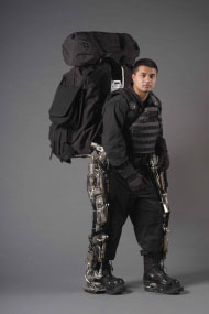
The BLEEX project has been an ongoing research at the University of California for a number of years and two versions currently exist. The motivation behind the project is to augment human strength. The device could potentially be used by fire fighters, disaster relief workers, and soldiers to carry heavier loads, further than otherwise possible (Figure 7.2).

The device is powered by hydraulic actuators at the hip (flexion and extension), knee (flexion) and ankle (plantarflexion and dorsiflexion¹) along the sagittal plane. Sensors mounted on the soles provide force feedback [HUA 05, KAZ 05].

However as BLEEX was designed to be used by an able-bodied person, the control architecture is structured so as to minimize impedance to the human user. There are no algorithms implemented to control postural stability, this has to be managed solely by the user. The sole purpose of the system is to bear the additional load on the user. Autonomous operation is achieved through a small fuel engine that powers the hydraulic components and the onboard computer.

7.1.2.3. Pneumatically powered knee-ankle-foot orthosis (KAFO) — University of Michigan

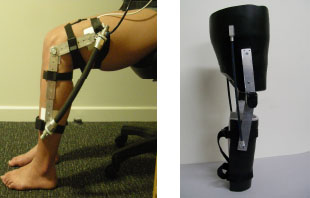
In an effort to understand the effects of a powered exoskeleton on normal human gait, pneumatically powered knee-ankle-foot (KAFO) [SAW 09] and ankle-foot orthosis (AFO) [FER 05, SAW 05] were developed at the University of Michigan. The research which spans for almost a decade now is centered on the application of torque (through pneumatic artificial muscles (PAM)) across the ankle and knee joints (Figure 7.3).

The orthoses were constructed from carbon fiber shells to custom fit the user’s leg [GOR 06, FER 06]. Surface electromyography (sEMG) signals from the tibialis anterior² and soleus³ were used as control signals for ankle dorsiflexion and plantar flexion in the AFO. In addition to the sEMG signals from muscles at the ankle, sEMG from the vastus lateralis and medial hamstrings were used for knee extension and flexion in the KAFO. The PAM force delivered was proportional to the rectified and filtered sEMG signals (i.e. proportional myoelectric control).

The latest publication on the research concluded that while the powered exoskeleton (AFO) delivered about 63% of the average ankle joint mechanical power during walking, this did not result in a proportional reduction of net metabolic power (about 10%). The authors suggest that metabolic savings when using a powered exoskeleton are less in joints with considerable elastic compliance (as in the ankle joint). Larger metabolic savings may be possible in joints that rely on power production due to positive muscle work, such as in the knee joint [SAW 08].

7.1.2.4. Hybrid assistive leg (HAL)

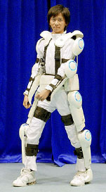
Another long standing research carried out by the University of Tsukuba (Japan) in cooperation with Cyberdyne Systems Company, is the hybrid assistive leg (HAL) project. The HAL suit is a wearable robot designed for human strength augmentation and to increase the quality of life for the elderly (Figure 7.4). More recently the work has been extended to provide walking motion support for persons with hemiplegia and gait rehabilitation for persons with incomplete spinal cord injury [KAW 09].

The exoskeleton is powered by dc servo drive motors at the hip and knee joint and in HAL 5 the elbow and shoulder joints are also powered. Various control systems have been developed to guide the movements of the exoskeleton with respect to the human user. The first exoskeletons utilized EMG feedback from the extensor muscles to determine the operator’s intentions [KAW 03b]. Later phase sequence algorithms were utilized to move the exoskeleton through a predefined motion based on the intention of the operator [KAW 04, KAW 03a]. A hybrid controller incorporating both the biological signals from the operator and motion information proved to be the most effective means of matching the viscoelasticity of the HAL suit to that of skeletal muscle [HAY 05].

To date, the HAL exoskeleton is recognized as one of the very few mobile, powered exoskeletons that are commercially available. However, research is still being carried out to diversify the application of the HAL suit [KAW 09].

This review of powered exoskeleton research is obviously not an exhaustive list of the research that is currently being carried out; however, those highlighted here have an immediate relation to the work that will be discussed in this chapter. Much inspiration has been drawn from the HAL project and the research at the University of Michigan.

7.1.2.5. Actuators for lower limb exoskeleton

There are various constraints imposed on a powered lower limb assistive device. The weight, type of actuator, power supply, range of motion, safety, low impedance and duration of use all play crucial roles. Common types of actuators utilized are electric (DC), hydraulic, and pneumatic drives. Each of these possesses its own advantages and disadvantages.

The electric drives (servo motors) have the advantage of being low cost, relatively easy to attain position and velocity control, and produce very low noise during operation [LOW 06]. On the other hand, the power and torque-to-weight ratio of a servo motor is significantly lower when compared with other types of actuation [CAL 95]. The main drawback of electric drives is the lack of compliance in the actuator. This last characteristic is of considerable importance as it affects the safety of the user. In [PRA 04] an electric servo motor is used in the construction of a series elastic actuator. Low impedance is achieved in this device through complex gearing.

Hydraulic actuators are generally more suitable for an industrial setting due to the high power-to-weight ratio, strength, and rigidity. The last two characteristics though ideal on the shop floor, are not suitable in an AR exoskeleton. Furthermore, hydraulic actuators suffer from high maintenance cost and the possibility of oil leaks.

Conversely, pneumatic actuators whilst possessing a similar high power-to-weight ratio, do not come with the maintenance and leakage issue that exist in hydraulic actuators. Pneumatic actuators are low in cost, have fast response time, and are inherently compliant and backdrivable, thus proving to be a good choice where there is human interaction [DAE 02].

Pneumatic artificial muscles (PAM) manage to provide an excellent “hybrid” that inherits the compliancy and backdrivability of a linear pneumatic actuator but not the weight and bulk. PAM’s are therefore ideal for powered AR exoskeletons.

PAM actuators have already been utilized since the 1950s in many AR devices [TON 00]. A significant portion of the research however concerns robotic locomotion, while these are not directly related to this work they do demonstrate the potential of PAM actuators [LIL 03, PAC 97, TAK 06]. The only significant drawback of the PAM actuator is the nonlinearity inherent in the system due to its construction and the compressibility of air. Classical control methods lack the ability to accurately manipulate the actuator. The modeling and control of the PAM actuator therefore is our focus and will be discussed in greater depth in the following sections.

7.2. Overview of knee exoskeleton system

The contribution of this work is the design and development of a pneumatic assistive knee exoskeleton. The basic principle behind the operation of the exoskeleton is the augmentation of the skeletal muscle force produced by the user. The fundamental control architecture of the exoskeleton is depicted in Figure 7.5.

Surface myoelectric signals from the knee extensor and flexor muscles provide the control link between the user and the exoskeleton. The sEMG signals are obtained through six bipolar electrodes attached to front and rear of the thigh. A preamplifier circuit mounted on the electrode conditions the signals before it is fed into a mapping algorithm. The purpose of the algorithm is to determine the degree of force exerted by the skeletal muscle and calculate the appropriate PAM force depending on the set assistance ratio. The encoder mounted on the exoskeleton provides kinematic feedback of the knee joint.

The force difference between the muscle and the PAM is provided as the reference signal to the motion controller. A multiple-input single-output self-organizing fuzzy controller is utilized as the motion controller. The inputs to the controller are the error (e) and the change in error (ė), and the output is the duty cycle of the PWM pulse.

The output from the motion controller regulates the valve opening of a high-speed (on/off) pneumatic solenoid valve. This is accomplished by varying the duty cycle of the 100Hz PWM pulse. Through this method the mass flow rate of air flowing into the PAM can be accurately controlled. Two valves are used to control the flow of air into the PAM, one for inflation and the other for deflation.

It is important to mention that the current exoskeleton design does not include any algorithms to ensure postural stability or to determine the user’s complete intended motion (e.g. sit-to-stand or ascending a flight of stairs). The PAMs are intended to operate in parallel to their organic counterparts and as such they augment rather than direct the movement. Since the basic control signal is derived from the sEMG signals, the high level controller in this exoskeleton system is the human motor system (cerebral cortex-brain stem-spinal cord), whereas the low level controller is the PAM motion controller.

Research conducted at the University of Michigan (section 7.1.2.3) has demonstrated that the human motor system is capable of changing muscle activation pattern in response to external support provided during walking. The objective therefore is to allow the motor system to control the coordination of the intended trajectory while the exoskeleton provides the assistance needed to do so. In this sense the exoskeleton is a seamless extension to the human motor system.

The control block diagram of the exoskeleton is illustrated in Figure 7.6, for the first and second generation knee exoskeleton prototypes, shown in Figure 7.7. The following sections in this chapter will elaborate on the various components of the exoskeleton as shown in the block diagram.

7.3. Modeling and control of pneumatic artificial muscle (PAM)

7.3.1. Background

The pneumatic artificial muscle otherwise known as the Mckibben muscle is a variant of the traditional pneumatic actuator. The invention of the muscle is attributed to Joseph L. Mckibben who in the 1950s utilized it to actuate an arm orthosis [SCH 61]. After initial popularity the actuator fell out of favor as electric drives rose in popularity in the 1960s. In the 1980s, the Japanese tire manufacturer Bridgestone reinvented a more powerful version of the PAM for a painting application called rubbertuator [INO 88]. However in the past decade there has been a renewed interest in the PAM actuator [ANH 08, BAL 03, BON 09, CHO 06, MIN 97, PAC 97, SIT 08, XIA 08] as a result of its inherent compliance and its properties that mimic skeletal muscle.

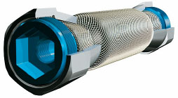
The Mckibben muscle falls under the category of braided muscles which essentially are an inflatable membrane enclosed within a braid. The sleeve or braid is a helical mesh that runs the length of the PAM. The PAM operates at an overpressure, that is the PAM exerts force on a load when supplied with compressed air (usually about 400–600 kPa). When pressurized the inner gas-tight elastic tube expands radially exerting force on the braid. The tension in the braid fiber balances the force exerted and this tension is summed at the endpoints of the PAM. The force then can be transferred to an external load. A CAD model of the internal construction of the PAM is given in Figure 7.8.

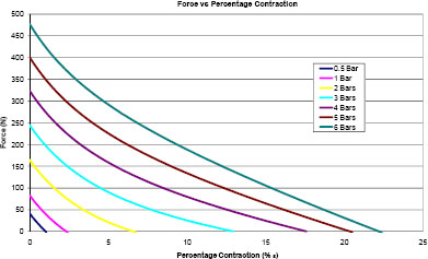
Early researches have opted to construct their own muscles based on the general design of the PAM; the problem that soon arises from this is the inability to reliably reproduce the characteristics of each PAM. To avoid this issue we have opted to utilize a commercially available muscle. One manufacturer of commercial PAM is the German company FESTO. They produce Mckibben muscles of various diameters (5 mm, 10 mm, 20 mm, and 40 mm) with known force and pressure characteristics (Figure 7.9). This type of PAM is capable of a maximum contraction of up to 25% of its original length. The detail characteristic data provided by the manufacturer provides a good foundation for further work.

7.3.2. Characteristic of the PAM

The ability of the PAM to inflate during contraction whilst maintaining a general cylindrical shape is the result of bias angle in the helical braid. The bias angle or braid angle is the angle between the PAM axis and the braid thread. By employing a weak enough initial angle the braid allows the expansion of the inner tube under pressure thereby converting circumferential pressure to axial force [TON 00].

Daerden and Lefeber [DAE 02] conducted two simple experiments to examine the operation of the PAM in which a PAM was fixed vertically at one end and had a mass hanging from the other end. In the first experiment the hanging mass was kept constant and the pressure within the PAM was gradually increased. In the second experiment the pressure within the PAM was kept constant and the mass was gradually reduced. The experiments led Daerden to propose rules to describe the behavior of the PAM:

1. The contraction of the PAM is realized by increasing its volume.

2. Contraction against a constant load can be achieved by increasing the pneumatic pressure within the PAM.

3. As the loading on a PAM is decreased, its contraction will occur at a constant pressure.

4. The contraction of the PAM has an upper limit at which point it reaches its maximum enclosed volume and exerts zero pulling force.

This last characteristic is of particular interest because in traditional linear pneumatic drives the force exerted is only proportional to the piston cross-sectional area and the pressure within the piston chamber. However in a PAM the force exerted is proportional to both the pressure and the muscle contraction.

PAMs possess many characteristics that are desirable in an exoskeleton actuator. The power-to-weight ratio of most PAMs is in the order of kN/kg. The PAM that is utilized in this work (MAS-10-N290) has a force-to-weight ratio of approximately 3.5 kN/kg [FES 03]. PAMs also exhibit inherent compliance and naturally damped dynamic response. The compliance is the direct result of the compressibility of air and the elasticity of the inflatable membrane while the damped response is due to the nonlinear kinetic friction intrinsic in the outer braid [DAE 02]. This compliant behavior is highly useful where there is close human-machine interaction.

Additionally, PAMs also bear a close resemblance to human skeletal muscle. Both are contractile actuators only capable of attractive forces and require an antagonistic setup for bidirectional motion. The decreasing force-contraction characteristic seen in PAMs is similar to the force-contraction characteristic in skeletal muscle. These attributes together with the intrinsic compliance make PAM an ideal extension to the human skeletal muscle.

7.3.3. Models from literature

The compressibility of air and the hysteresis in the PAM actuator result in a highly nonlinear system that is difficult to both model and control. Researchers [DAE 02, MIN 10, TON 00] have attributed the hysteresis losses to thread-on-thread dry friction acting within the PAM braided shell, the friction between the braid and the inner bladder, and the hysteresis of the inner bladder itself.

As a result many models have been developed to approximate the properties of the PAM. Two common models used in literature will be discussed. The first is based on the principle of virtual work and the geometry of the PAM braid [CHO 96, TON 00].

Assuming that the PAM maintains its cylindrical shape during contraction, the principle of virtual work can be applied to determine the force exerted. As the PAM contracts its radius increases from r₀ to r and its length decreases from l₀ to l. Assuming positive motion in the direction of muscle extension, the virtual work of the pressure force can be expressed by:

[7.1] 

where V is the change in volume as the result of the increase in radius. Taking into account the current braid angle a, the expression of F, the force exerted by the PAM as a function of the control pressure P and the contraction ratio ε (l₀/l) is shown to be:

[7.2] 

The model shows the change in force exerted by the PAM; at zero contraction the force is maximum and at maximum contraction the force falls to zero.

The model derived from virtual work requires prior knowledge of the braid angle; it is however impossible to determine the braid angle in a commercial muscle such as the one that has been utilized in the work. It is therefore necessary to take another approach to model the PAM. Situm and Herceg [SIT 08] have modeled a similar PAM from the same manufacturer by approximating the response with a first order lag term. The transfer function is defined as the ratio of the pressure in the actuator to the control signal of the proportional pneumatic valve.

[7.3] 

The transfer gain K_m and the time constant T_m are determined experimentally. The pressure is then related to the force exerted based on a physical static model without weave geometries. This equation expresses the force developed by the PAM as a function of only the pressure and contraction ratio.

[7.4] 

where l_max and l_min are the relaxed and fully contracted muscle length. The constant K_p which is dependent on the working pressure P is determined experimentally.

The static models described do not take into account the hysteresis inherent in the PAM. Often the hysteresis in the PAM is not explicitly modeled but grouped together as part of the nonlinearity in the actuator. In a recent work by Minh et al. [MIN 10] the hysteresis in the PAM is explicitly modeled using a Maxwell slip model and used in a feed forward compensator in the control loop.

7.3.4. Model used

In this work the PAM is modeled as a quasi-static system with the hysteresis incorporated into the nonlinear characteristic curve of the actuator. The main motivation to model the PAM was to enable the offline tuning of the self-organizing fuzzy controller. It is important to note here that the modeling of the pneumatic subsystems is not essential for the fuzzy controller. The controller is fully capable of tuning itself online as the system operates. However, as a preliminary step the offline (simulation) tuning of the controller was performed to evaluate the performance of the controller. Thus it was necessary to obtain models of the subsystem (PAM-high speed valve-air mass flow rate) to perform simulation. The utilization of the models for the offline tuning of the fuzzy controller will be described in section 7.5.4.

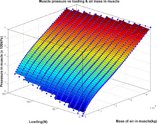
To obtain an empirical approximate model of the PAM, look-up tables instead of a mathematical model is used. It is known from the literature that the force developed by the PAM is proportional to its percentage contraction (%ε) and the pressure in the PAM. The pressure and percentage contraction in the PAM is in turn proportional to the mass of air in the PAM and the loading on it. Therefore it follows that if the mass of air in the PAM and the loading is known at all times then the %ε and the force exerted by the PAM can be determined.

The experimental data points for the look-up table were obtained by attaching a fixed load on the PAM and increasing the pressure within the PAM at set increments. The %ε and the volume of air in the muscle (the PAM is approximated to a cylinder and the volume of air contained within is calculated) for each increment in pressure were recorded. The entire procedure is repeated with the loading increased from 0–150 N at 10 N increments. The experiment carried out is similar to those conducted by Daerden and Lefeber that was mentioned earlier.

The reason the PAM data was obtained experimentally rather than by simply using the data provided by the manufacturer is first to acquire the necessary additional information regarding the mass of air in the PAM at different pressures and to also verify the data provided by the manufacturer. The first table (here shown as a 3D surface, Figure 7.10) relates the pressure within the PAM to the mass of air in the PAM and the loading.

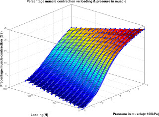
By means of these two characteristic curves the %ε of the PAM and the pressure within the PAM can be determined if the mass of air entering the PAM is known. The modeling of the pneumatic valve to determine the mass flow rate will be discussed in section 7.4.

The second surface (Figure 7.11) relates the %ε of the muscle to the pressure within the muscle and the loading. The force can then be calculated as a function of %ε and pressure.

7.4. Modeling of high-speed on/off solenoid valve

In literature the most prevalent way to regulate the pressure within the PAM is through a proportional pressure regulator. The regulator provides a simple and easy means to control the pressure within the PAM by varying the voltage or current. However, pressure regulators are often expensive, bulky, and require constant power supply to function.

Another method proposed in literature is to pulse a high-speed solenoid valve to vary the valve opening [BAR 97, CHE 07, SIT 08, ZHA 08]. The flow equation relating the valve orifice area, A_V to mass flow rate, is:

[7.5] 

In this experiment the valve orifice is assumed to be a circle, which is a close approximation of the shape of the orifice and C_f is a non-dimensional discharge coefficient through the orifice. κ is the ratio of specific heats. The mass flow rate is also dependent on the ratio of the pressure before (P_u, upstream pressure) and after the orifice (P_d, downstream pressure). The orientation of the P_u and P_d change depending on whether the PAM is inflating or deflating. During inflation, P_u is the supply pressure of 600 kPa and P_d is the increasing pressure within the PAM. During deflation the opposite is true, P_u is the decreasing pressure within the PAM and P_d is the constant atmospheric pressure.

The constants C₁, C₂, and the critical pressure P_cr are calculated as equation [7.6]. For the PAM system the critical pressure ratio P_cr for the system is P_cr = 0.528.

[7.6] 

Two high-speed 3/2 way solenoid valves (FESTO MHE2-MS1H-3/2G) with a switching time of approximately 2 ms are used to adjust the orifice opening, and control the pressure within the PAM. One valve is responsible for inflating the PAM and the other is used to deflate the PAM. Thus the valves are in fact used as 2/2 way valves with the exhaust port plugged.

The maximum operating frequency of this valve is 330 Hz (3 ms pulse period); however since the minimum valve switching time is 4 ms the operating frequency was set to 100 Hz (10 ms pulse period). This frequency was chosen to provide a gradual increase in flow rate with regard to the PWM duty cycle. At high frequencies the operation of the high-speed valve is subject to complex electric and magnetic influences. Electrical delay, magnetic delay, and mechanical delay all combine to retard the response of the valve [KAJ 95].

An intuitive attempt to model the dynamics of the on-off valve is proposed by Chen et al. [CHE 07]. The initial model is here adapted and extended to encompass all the possible states of the valve. The initial model is given in equation [7.7] and graphically depicted in Figure 7.12.

[7.7] 

where X_i is the spool displacement, X_m the maximum spool displacement, U PWM pulse magnitude, i the number of PWM pulses starting from 1, 2, 3…n, T_c the PWM period, T_p the PWM on period, t₁ electrical delay and magnetic delay (armature picking up time, approx 1 ms), t₂ mechanical delay (spool responding time, approx 1 ms), t₃ electrical delay and magnetic delay (armature take down time, approx 1 ms), t₄ mechanical delay (spool release time, approx 1 ms). The switching on and off time are given by t₁+ t₂ (2 ms) and t₃+ t₄ (2 ms).

The equation given however is only applicable when (t₁+t₂) ≤ T_p≤ (T_c-t₃-t₄). In this work this state is referred to as the third state (out of five). To accommodate other possible states four other switching modes were identified and modeled. These states are dependent on the PWM period, and model the characteristics when the PWM period is either too short so that the spool will not fully extend or too long, preventing the full return of the valve spool.

7.4.1. Experimental validation of high-speed valve flow rate

The flow rate profile of the high-speed valve with PWM control that was obtained through simulation (shown in Figure 7.13) was experimentally verified. Data obtained through simulation illustrates the dead band and the saturation that occurs within the high-speed valve at low and high duty cycles respectively.

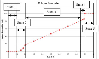
The experimental setup to verify the simulation data was carried out using a (MHE2-MS1H-3/2G) valve and a flowmeter (Platon NG). The results obtained show that the model overestimates the flow linearity and maximum flow rate (Figure 7.14). However, the dead band and saturation of the valve are evident from the graph; the discrepancy in the linearity may possibly be due to nonlinear flow profile through the orifice. To better reflect the actual valve flow profile, the discharge coefficient and the maximum valve opening in equation [7.5] were readjusted.

7.5. Self-organizing fuzzy control

7.5.1. Introduction to fuzzy control

Fuzzy control is the offspring of fuzzy set theory proposed by Lofti A. Zadeh in the 1960s and 1970s [ZAD 65, ZAD 68]. It essentially is a method of intelligent control based on human heuristic knowledge. In fuzzy logic a set is said to have varying degrees of truth ranging from 0 to 1. This is in contrast to the traditional Boolean logic of either 0 or 1. In fact, Boolean logic can be seen as a boundary form of fuzzy numbers and sets.

In everyday life, most things are described with linguistic variables and modifiers. As an example the linguistic variable height can have linguistic values of short, medium, and tall, and can be modified with, slightly, very, and extremely. These variables do not have a defined boundary, or in other words are “fuzzy”. Figure 7.15 gives the fuzzy representation of the set of tall men. The universe of discourse (x axis) contains all the elements that are considered, in this case the height of men.

When applied to control systems, fuzzy logic has the capability to accurately control highly nonlinear systems [JAN 98, KOV 06]. The decision-making process in a fuzzy control system is based around the very common IF-THEN statement.

IF the input is X, THEN the output is Y.

This structure is highly suitable to capture the experience and knowledge of a human operator. These IF-THEN rules are stored in an inference engine and executed based on the input to the system. As a result fuzzy control is an effective tool when dealing with ill-defined systems where the mathematical modeling is poor [JAN 98c, KOV 06]. The fuzzy inference engine operates based on expert human knowledge and experience in place of a detailed model. The complete concept of fuzzy control will be explained with respect to the PAM control system.

7.5.2. Fuzzy control system for PAM

First the input and output variables of the fuzzy controller is defined. The fuzzy control system for the PAM is based on a PD-type controller. The input to the controller is the error (e) and the differential of the error (ce). The error is the difference between the reference force and the force generated by then PAM. Figure 7.16 gives the simplified overview of the control system.

The output of the fuzzy controller is the duty cycle (u) of the PWM generator which will in turn regulate the air flow into the PAM. This will enable accurate control of the pressure within the PAM and thereby the force exerted by the PAM. The output duty cycle ranges from −100% (for deflation of the PAM) to 100% (for PAM inflation).

Both input variables and the output variable (Figure 7.17) have seven membership functions in the fuzzy set, over the universe of discourse (−1 to 1). In the case of the output fuzzy set, −1 corresponds to −100% deflation and the opposite, for inflation. The linguistic values [(B)ig, (M)edium, (S)mall, and (Z)ero] modify the (P)ositive and (N)egative input values. Each linguistic value is represented as a membership function. A function that ties each element of the universe to a membership value is called a membership function. The membership functions are biased toward the center to give better control when the error or change-in-error is close to equilibrium.

Triangular membership functions are used for the middle membership functions, while trapezoidal ones are used at the two ends. This is the standard and well-established method for an initial fuzzy controller design [JAN 98]. Although the universe is the same for both input variables, the input gains for each variable can be adjusted to give better system response [JAN 98].

The output membership functions have similar shapes to that of the input variables; however, the central function is a trapezoid instead of a triangle to account for the dead band of the high-speed pneumatic valve.

Next, the fuzzy rule base is built based on expert knowledge of the system that is to be controlled. In the case of the PAM, existing rule base from literature is adapted to suit the requirements of the system [CHE 07, MIN 97, ZHA 08]. The rule base used for the fuzzy controller is given in Table 7.2.

Since there are seven membership functions in each input variable, there is one rule for each input combination to ensure that for every possible input combination there is a rule to determine the appropriate action. As an example, referring to Table 7.2 — IF the error is NB (negative big) AND the change in error is PS (positive small) THEN the output duty cycle is NM (negative medium). This rule can be simplified to:

 

Finally the fuzzy inference engine evaluates the fuzzified inputs based on the rule base and provides a crisp output.

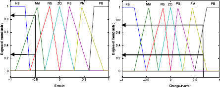
The operation of the fuzzy inference engine can then be demonstrated using a simple example. In Figure 7.18 two arbitrary input variables are assumed (e = −0.5, ce = 0.6). The crisp inputs firstly undergo a fuzzification process. The crisp error input is fuzzified and has about 0.22 degree of membership to the set of NS and 0.82 to the set NM. The crisp change-in-error input is also fuzzified and has degrees of membership of 0.22 to the set PM and 0.66 to the set PB.

This causes all rules with the corresponding membership functions to fire. The combinations of rules that will fire are highlighted in gray in Table 7.2. The firing strength of the rule is determined by the AND method, in this case since the rules are:

 

where u_e1 and u_ce1 are the respective activation levels, the min operator is used. The operator sets the activation of the antecedent part of the rule equal to the lower activation of the two terms.

The deduction of consequent or the conclusion of the rule (THEN…) is called fuzzy implication. The min operator is used here also. This operator clips the output (consequent part) membership function based on the activation level of the antecedent part. If more than one rule fires for a given input combination, as in this case, all the clipped consequent parts have to be combined before a crisp output can be determined. This operation is called fuzzy aggregation. The max operator used for the aggregation will produce an output fuzzy set based on the maximum activation of each output membership function. The final step is the defuzzification for the output fuzzy set into a crisp output. The centroid of area method is used for this purpose:

[7.8] 

where µ(x_i) is the membership value in the membership function and x_i is a running point the continuous universe. The function calculates the output as the weighted average of the elements in the output set [JAN 98, KOV 06]. Figure 7.19 shows the fuzzification, activation, implication, and defuzzification of the four rules from the example (e = −0.5, ce = 0.6). The crisp output from the controller is a duty cycle of 0.2 (20% PAM inflation).

Once the fuzzy inference engine has been designed it is then possible to determine the crisp output for all possible input combinations. This can be represented in the form of a surface known as the fuzzy control surface. The control surface for the PAM is given in Figure 7.20.

However, for control application it is often better to discretize the input universe to achieve faster computational speed. Thus the inputs into the fuzzy controller are quantized to increments of ±0.05; this allows the fuzzy control surface to be simplified to a 41 × 41 look-up table. The look-up table then can easily be incorporated into the feed-foward path of the control loop to achieve fast control response.

7.5.3. Introduction to self-organizing fuzzy controllers

The adjustment of the fuzzy membership functions and the rule base is often based on heuristics and expert knowledge. This method though often sufficient does not necessarily always result in a controller that is optimized to affect the desired response for a particular plant. The alternative approach proposed by Mamdani in his pioneering papers [MAM 75, PRO 07] is a fuzzy logic controller that is capable of self-organization iteratively based on the control quality and the desired response of the plant.

One basic structure of a self-organizing controller is a lower level standard- table-based fuzzy controller and a higher level adjustment mechanism (Figure 7.21). The higher lever modifier corrects the values in the table of the lower controller if the current performance does not match the desired.

If the current performance is as desired then the modifier does not have to correct the values in the table; however, if the performance is inadequate then a particular entry in the table has to be adjusted to give the correct control signal. The modifier cannot and should not penalize the current table entry (for current plant output) as there is a delay between the control output and the plant response. A simplification proposed by Jantzen [JAN 98b] is to correct the control output that occurred in a few samples in the past. The number of samples or the delay-in-penalty “d” corresponds to the time lag of the plant. The modification in the fuzzy table can be expressed as:

[7.9] 

where i is the current iteration and ∆P_i is the correction factor added to the entry in the table-based controller. From the equation it is evident that this modification algorithm will only succeed if the increase in the control signal corresponds to an increase in the plant output and vice versa. Fortunately this is the case in the PAM system.

7.5.4. Practical implementation

In theory the lower fuzzy table-based controller can initially be zeros and the modifier algorithm should be able to generate the fuzzy table iteratively. Nonetheless, if the fuzzy table is already populated with reasonable values (as described in section 7.5.20) the convergence of the self-organizing fuzzy controllers (SOFC) is considerably faster.

Traditionally the modifier algorithm determines the correction factor ∆P_i, based on a performance table [PRO 07]. The performance table is basically a two dimensional look-up table similar to the fuzzy control table. The table represents the desired transient behavior of the plant. Thus a performance table designed for one plant could easily be used for another as it only represent the desired behavior. A practical simplification of this is a penalty equation proposed by Jantzen [JAN 98b] to replace the performance table.

[7.10] 

The correction factor is a function of the learning gain G_p, the desired time constant τ, and the sample period Ts. The learning gain effects the rate of convergence. Too small and the SOFC will take a long time to converge if at all, too large and the system will become unstable rapidly. Jantzen proposes rule of thumb equations to govern the selection of τ and G_p. The desired time constant should be bounded by the plant time constant, τ_p, and dead time, T_p.

[7.11] 

The original equation states that G_p should be chosen so that each correction factor is not greater than 1/5 of the maximum value in the fuzzy table. This prevents the fuzzy table from winding up and causing the system to become unstable. Based on experimentation it was concluded that a magnitude of 1/10 produced better results.

The SOFC was initially trained offline to assess the quality of the trained controller compared to the standard fuzzy controller. The training was carried out in MATLAB Simulink environment. The entire PAM system had to be modeled to enable offline training. Figure 7.22 shows the Simulink SOFC block diagram.

In the final implementation an online training would be sufficient. The online training would negate the necessity to model any of the subsystems within the pneumatic system, and as such prove to be a more efficient solution when compared to model-based controllers.

The high-speed pneumatic valve model is included in the “valve-opening model” block. The two look-up tables to model the PAM are incorporated in the “muscle model” block and the “mass flow rate equation” block calculates the mass of air entering and leaving the PAM based on the valve opening and pressure difference (section 7.4).

7.5.4.1. Simulation training results

In order to properly train the SOFC offline, the reference input should match the reference input from the actual system; however, as this reference is to be derived from the exoskeleton user’s surface EMG signal a simplified reference was used (i.e. a sinusoid signal).

Prior to implementing a force control system (as would be implemented in the final exoskeleton), a position control system was implemented as a preliminary test of the SOFC performance. The feedback in this simulation was the percentage contraction of the PAM and the reference was the intended percentage contraction.

The SOFC was trained with a 2 Hz rectified sinusoid wave as this signal resembled the motion of the knee joint during normal walking movement. The frequency of 2 Hz was chosen as this was deemed to be the upper limit for the step frequency in a person requiring assistance (i.e. 2 steps per second per leg) [CHA 10]. The amplitude of the sine wave was set to 17% PAM contraction which is approximately 60^o knee flexion. Figure 7.23 shows the PAM tracking before training and Figure 7.24 shows the tracking after a training session of 80 seconds.

Simulation of the SOFC validates the ability of the modifier algorithm to improve the tracking accuracy of the fuzzy controller. The encouraging results obtained through simulation justify an experimental testing of the SOFC.

7.6. Surface electromyography

7.6.1. Origins of surface electromyography (sEMG) signals

The link between the user and the exoskeleton is achieved via surface myoelectric signals. These signals are intended to allow the user direct control of the exoskeleton and by this means provide intelligent control. The challenge however it to determine an exact mapping of the signals recorded on the skin surface to the muscle torque developed across the knee joint. This section is still part of an ongoing research and only preliminary findings are discussed. The sEMG origin, signal acquisition and processing, and sEMG to force mapping will be discussed in this chapter.

Muscles are both the dominant tissue and the primary organ of the human body. An estimated 70% to 85% of gross body weight is attributed to muscles [CRA 98]. Skeletal muscle, which is the type of muscle concerned here, produces torque across a joint by shortening its resting length. On a macroscopic level muscles are classified by their line of action, direction of pull and their origins⁴ and insertions.⁵ However closer investigation reveals that muscles are in fact composed of compartments. Thus instead of a unit of massive muscle, most muscles are made up of a series of smaller compartments that run along the same or different direction [CRA 98]. Muscles are surrounded by connective tissue that hold them together and prevent displacement from the line of action.

The functional unit of the neuromuscular system is the motor unit (MU). MUs consist of an α-motor neuron and the connected muscle fibers [STA 10]. The α-motor neurons, located in the spinal cord of the brain stem, creates an electrical impulse (action potential) that travels along axons to its terminal branches, each of which is connected to a single muscle fiber at the neuromuscular junction. The connection is usually in the middle or proximal to the middle. As the action potential (AP) reaches the muscle fibers, depolarization of the fiber membrane triggers muscle contraction. The membrane depolarization causes a time-varying transmembrane electric current field that can be measured non-invasively from the surface of the skin above the muscle [BAS 62].

Since a single action potential will only cause a twitch, to achieve a longer period of contraction a series of APs are generated by the motor neuron. The recruitment or firing of the muscle fibers is generally recognized to be random; however, studies have shown that smaller MUs located deep within the muscle are recruited first before larger MUs closer to the muscle surface are recruited [DAH 05].

The EMG signal detected on the skin surface is the algebraic summation of these APs [DAY 01]. As these waves are bi-phasic or trihasic, the phase cancelation that consequently occurs, results in the detected EMG signal having an amplitude less than proportional to the number of MU firing per second. The amplitude of the detected surface EMG also varies significantly as a result of the summation [KEE 08].

7.6.2. sEMG signal acquisition and conditioning

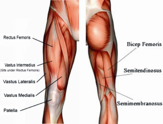
The muscle groups that are of interest for the present application are the knee extensor and flexor muscles. Three extensor and three flexor muscles were chosen based on their percentage cross-sectional area (%PCA) and the ability of signal detection using surface electrodes. The extensor muscles are vastus lateralis (20%), rectus femoris (8%) and vastus medialis (15%). The flexor muscles are semitendinosus (3%), semi-membranosus (10%), and biceps femoris (10%) (Figure 7.25).

Gold-plated bipolar electrodes were used in conjunction with a preconditioning circuit to preprocess the acquired sEMG signals. The preconditioning circuit layout is given in Figure 7.26. The instrumentation amplifier is essentially a high-input impedance differential amplifier with a high common mode rejection ratio. Next band pass filters (20–400 Hz) are utilized to section out the frequencies that have the most information (energy) regarding the muscle activation. A second amplifier is then used to further boost the signal to fall within the 0–5 V range. Thus the original signal is amplified 1,000 times.

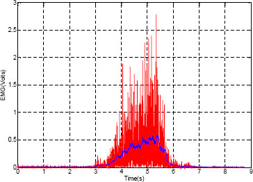
The preprocessed signal is sampled at 1,000 Hz, full wave rectified and then filtered using a moving average filter with a window of 100 values. Existing literature recommends low pass filtering at frequencies below 3 Hz to estimate the force envelope, however the phase delay (group delay) associated with classical filtering techniques is not desired in control applications. Physiologically there is a time delay between the onset of electrical activity and detection of force. This electromechanical delay (EMD) is estimated to range from 30 ms to 150 ms [STA 05], thus a moving average filter provides a constant delay (100 ms) within the EMD, which is not a function of the frequency (Figure 7.27 and 7.28).

7.6.3. Relating sEMG to muscle force

The processed sEMG signals next have to be related to the force generated by each muscle [HAY 09, FLE 04]. Various methods have been proposed for this purpose, most of which are primarily concerned with the exact modeling of the sEMG to force relationship. These methods usually are not practical in a real-time control scheme. In the case of a lower limb exoskeleton a close approximation will suffice as the assistance ratio can be adjusted to provide a “comfortable” support.

Proportional myoelectric control was implemented by Ferris et al. [FER 06] to control an ankle-foot orthosis. The acquired sEMG signal was first rectified and low pass filtered, then used to proportionally control the pressure within PAMs. This linear and simplistic approximation to the muscle force was sufficient for the intended tests. In his PhD thesis Fleischer [FLE 07] proposed a simplified biochemical body model to relate the acquired EMG to the force produced. The model was based on the traditional Hill type model which approximates each muscle group to a contractile element that creates active force in parallel with a passive element that resists stretching through passive force. The model developed displayed impressive results; however, certain key parameters such as the force-velocity correlation and the change of the optimal muscle fiber length with respect to the activation level were left out to reduce the number of parameters that needed to be calibrated each time. These crucial parameters could in theory improve the accuracy of the model.

In the current work, the preliminary control signals for the PAM actuators are derived from sEMG signals in a similar fashion to the method employed by Ferris et al., that is proportional myoelectric control. This initial setup will be replaced by an artificial neural network (ANN) model that would be able to capture the nonlinear relation between the knee angle (θ), knee velocity , the six sEMG signals, and the resultant torque across the joint. Similar works by Luh et al. [LUH 99] and Hahn [HAH 07] have demonstrated the viability and the effectiveness of such an approach.

7.7. Hardware implementation

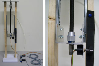
A real-time fuzzy control system was implemented to verify the results obtained through simulation. National Instruments compact RIO (NIcRIO-9074) together with LabVIEW graphical programming language were used as the real time hardware. The facility of FPGA (Field Programmable Gate Array) allowed fast and deterministic input sampling and control signal output. The input into the control system is the position from the encoder (US Digital S5S-360 pulse/rev) and the outputs are the PWM signals to the two high-speed valves. The PAM used for the experiment is the MAS-10-N290 (10 mm internal diameter and 290 mm relaxed length) from Festo Inc (Figure 7.29).

The experiment was carried out for the PAM position (percentage contraction) control. As mentioned in section 7.5.4.1, position control was implemented as an initial effort to ascertain the performance of a SOFC. The trained fuzzy surface was implemented directly into the LabVIEW code as a 2D array. The entire control algorithm could be executed within 2 ms and since the PWM period is 10 ms (section 7.4) this was well within the allocated time period.

The tracking accuracy of the controller was tested with step inputs. The ideal behavior would be for the PAM to minimize air losses as this is undesirable if it is to be implemented in a mobile orthosis. Thus a certain amount of undershoot is preferred to overshoot.

Three test inputs were used, step input of 5%, 10%, and 15% contraction. A loading of 4.55 kg was attached to the lower end of the PAM, to represent the leg weight. The test was repeated three times and the average steady-state error was calculated. The steady-state error for each contraction level is given in Table 7.3.

Table 7.3. Experimental steady-state error for various input signals

Input	Steady-state error (%)
5% contraction with 4.5 kg load	1.2
10% contraction with 4.5 kg load	1.76
15% contraction with 4.5 kg load	1.25
10% contraction with no load	0.07

The unloaded system response for a given reference input is much smoother (Figure 7.30) than a system with loading. The main reason for this is the inertia of the load and the spring-like characteristic of the PAM. The accelerated load compresses the PAM and causes the system to oscillate slightly (Figure 7.31). This behavior is only observed during a step reference input; however for ramp or sinusoid input the tracking is smoother.

The next step is to perform online training of the SOFC and to compare its performance with an offline-trained SOFC. If the online training proves to be successful then the assumption can be made that the offline training can be omitted when developing the force control system.

7.8. Concluding remarks

The design simulation and experimental validation of a self-organizing fuzzy controller to achieve accurate position control of a PAM for a lower limb exoskeleton is discussed. Simulation and experimental results justify the application of a fuzzy controller to control the highly nonlinear PAM pneumatic system. Though classical model-based approaches have been used in the literature to achieve PAM control, the facility with which the fuzzy controller is able to achieve comparable results is impressive.

When integrated with self-organizing capability the controller is able to quickly adapt the control surface to suit the controlled system. It is envisaged that the fuzzy force control system that will ultimately be implemented in the exoskeleton, will obtain similar performance results as those from the position control.

Similarly, it is hypothesized that artificial intelligence methods employed to map the nonlinear relationship between the force developed by the knee muscles (extensor and flexor) and the measured EMG signals will outperform model-based approaches in terms of simplicity. Neural networks are generally recognized to be an excellent universal approximator, thus this characteristic can be exploited to model the sEMG-force relationship.

In conclusion, the application of fuzzy logic and neural networks, along with a compliant and skeletal muscle-like actuator, is deemed to be an ideal combination for a powered lower limb exoskeleton.

7.9. Acknowledgment

The authors would like to acknowledge Mr Markus Dreher and Festo Inc. for providing the fluidic muscles (PAM) used in this research. The advice provided by Mr Campbell Lintott (Festo NZ) and Julian Murphy (University of Canterbury) is also acknowledged.

7.10. Bibliography

[ANH 08] ANH H.P.H., AHN K.K., IL YOON J., ICROS/kOMMA, “Identification of the 2-axes pneumatic artificial muscle (PAM) robot arm using double NARX fuzzy model and genetic algorithm”, International Conference on Smart Manufacturing Application, Goyangsi, South Korea, 9–11 April 2008.

[BAL 03] BALASUBRAMANIAN K., RATTAN K.S., “Fuzzy logic control of a pneumatic muscle system using a linearizing control scheme”, 22nd International Conference of the North-American-Fuzzy-Information-Processing-Society (NAFIPS) Chicago, Il, 24–26 July 2008.

[BAR 97] BARBER A., 1997, “Pipe flow calculations”, in Pneumatic Handbook, edited by E. S. Ltd, Oxford, Elsevier Advance Technology.

[BAS 62] BASMAJIAN J.V., “Muscles alive: Their functions revealed by electromyography”, Journal of Medical Education, vol. 37, no. 8, 1962, p. 802.

[BEE 07] WWW.BEEBLEBLOG.COM, “Diagram of hamstring muscles”, edited by B. s. F. Blog, 2007.

[BON 09] BONG-SOO K., KOTHERA C.S., WOODS B.K.S., WERELEY N.M., “Dynamic modeling of Mckibben pneumatic artificial muscles for antagonistic actuation”, IEEE International Conference on Robotics and Automation, 2009.

[CAL 95] CALDWELL D.G., MEDRANOCERDA G.A., GOODWIN M., “Control of pneumatic muscle actuators”, IEEE Control Systems Magazine, vol. 15, no. 1, 1995, pp. 40–48.

[CHA 10] CHANDRAPAL M., CHEN X., WANG W., “Self-organizing fuzzy control of pneumatic artificial muscle for acitve orthotic device”, 6th IEEE Conference on Automation Science and Engineering, Toronto, Canada, August 2010.

[CHE 07] CHEN Y., ZHANG J.F., YANG C.J., NIU B., “Design and hybrid control of the pneumatic force-feedback systems for arm-exoskeleton by using on/off valve”, Mechatronics, vol. 17, no. 6, 2007, pp. 325–335.

[CHO 96] CHOU C.P., HANNAFORD B., “Measurement and modeling of McKibben pneumatic artificial muscles”, IEEE Transactions on Robotics and Automation, vol. 12, no. 1, 1996, pp. 90–102.

[CHO 06] CHOI T., LEE J., LEE J., “Control of artificial pneumatic muscle for robot application”, Proceedings of the 2006 IEEE/RSJ International Conference on Intelligent Robots and Systems, Beijing, China, 9–15 October 2006.

[CRA 98] CRAM J.R., KASMAN G.S., HOLTZ J., Introduction to Surface Electromyography, 1st edition, Gaithersburg, Maryland, Aspen Publication, 1998.

[DAE 02] DAERDEN F., LEFEBER D., “Pneumatic artificial muscles: Actuators for robotics and automation”, European Journal of Mechanical and Environmental Engineering, vol. 47, 2002, p.10.

[DAH 05] DAHMANE R., DJORDJEVIC S., SIMUNIC B., VALENCIC V., “Spatial fiber type distribution in normal human muscle: Histochemical and tensiomyographical evaluation”, Journal of Biomechanics, vol. 38, no. 12, 2005, pp. 2451–2459.

[DAY 01] DAY S.J., HULLIGER M., “Experimental simulation of cat electromyogram: Evidence for algebraic summation of motor-unit action-potential trains”, Journal of Neurophysiology, vol. 86, no. 5, 2001, pp. 2144–2158.

[FER 05] FERRIS D.P., CZERNIECKI J.M., HANNAFORD B., “An ankle-foot orthosis powered by artificial pneumatic muscles”, Journal of Applied Biomechanics, vol. 21, no. 2, 2005, pp. 189–197.

[FER 06] FERRIS D.P., GORDON K.E., SAWICKI G.S., PEETHAMBARAN A., “An improved powered ankle-foot orthosis using proportional myoelectric control”, Gait Posture, vol. 23, no. 4, 2006, pp. 425–428.

[FES 03] FESTO A.G., CO KG, “Fluidic muscle DMSP, with press-fitted connections & fluidic muscle MAS, with screwed connections”, Info 501, edited by F. A. C. KG, Festo AG & Co. KG, 2003.

[FES 10] FESTO A.C., 2010, “Fluidic muscle”, Festo AG & Co., 2010 [cited 14 December 2010]. Available http://www.festo.com/rep/el_gr/assets/Corporate_img/Fluidicmuscle_0375mu_500px.jpg.

[FLE 04] FLEISCHER C., KONDAK K., REINICKE C., HOMMEL G., “Online calibration of the EMG to force relationship”, Proceedings of the 2004 IEEE/RSJ International Conference on Intelligent Robots and Systems (IROS 2004), 28 September–2 October, 2004.

[FLE 07] FLEISCHER C., “Controlling exoskeletons with EMG signals and a biomechanical body model”, Faculty IV — Electrical Engineering and Computer Science, Technical University of Berlin, Berlin, 2007.

[GOR 06] GORDON K.E., SAWICKI G.S., FERRIS D.P., “Mechanical performance of artificial pneumatic muscles to power an ankle-foot orthosis”, Journal of Biomechanics, vol. 39, no. 10, 2006, pp. 1832–1841.

[HAH 07] HAHN M.E., “Feasibility of estimating isokinetic knee torque using a neural network model”, Journal of Biomechanics, vol. 40, no. 5, 2007, pp. 1107–1114.

[HAY 05] HAYASHI T., KAWAMOTO H., SANKAI Y., “Control method of robot suit HAL working as operator’s muscle using biological and dynamical information”, Proceedings of the 2005 IEEE/RSJ International Conference on Intelligent Robots and Systems, (IROS 2005), 2005.

[HAY 09] HAYASHIBE M., GUIRAUD D., POIGNET P., “EMG-to-force estimation with full-scale physiology based muscle model”, Proceedings of the 2009 IEEE/RSJ International Conference on Intelligent Robots and Systems (IROS 2009), 10–15 October 2009.

[HOO 09] HOOTMAN J.H.C., THEIS KA, BRAULT MW, ARMOUR BS, “Prevalence and most common causes of disability among adults — United States, 2005”, Morbidity and Mortality Weekly Report, MMWR, vol. 58, no. 16, 2009, pp. 421–426.

[HUA 05] HUANG L.H., STEGER J.R., KAZEROONI H., “Hybrid control of the berkeley lower extremity exoskeleton (BLEEX)”, ASME International Mechanical Engineering Congress and Exposition, Orlando, FL, 5–11 November 2005.

[INO 88] INOUE K., “Rubbertuators and applications for robots”, The 4th International Symposium on Robotics Research, Cambridge, MA, 1988.

[JAN 98] JANTZEN J., Design of fuzzy controllers, DK-2800 Lyngby, Denmark, Technical University of Denmark, Department of Automation, 1998.

[JAN 98b] JANTZEN J., The self-organising fuzzy controller, DK-2800 Lyngby, Denmark, Technical University of Denmark, Department of Automation, 1998.

[JAN 98c] JANTZEN J., Tutorial on fuzzy logic, DK-2800 Lyngby, Denmark, Technical University of Denmark, Department of Automation, 1998.

[KAJ 95] KAJIMA T., KAWAMURA Y., “Development of a high-speed solenoid valve — investigation of solenoids”, IEEE Transactions on Industrial Electronics, vol. 42, no. 1, 1995, pp. 1–8.

[KAW 03a] KAWAMOTO H., KANBE S., SANKAI Y., “Power assist method for HAL-3 estimating operator’s intention based on motion information”, Proceedings of the 12th IEEE International Workshop on Robot and Human Interactive Communication (ROMAN 2003), 2003.

[KAW 03b] KAWAMOTO H., SUWOONG L., KANBE S., SANKAI Y., “Power assist method for HAL-3 using EMG-based feedback controller”, IEEE International Conference on Systems, Man and Cybernetics, 2003.

[KAW 04] KAWAMOTO H., SANKAI Y., “Power assist method based on phase sequence driven by interaction between human and robot suit”, Proceedings of the 13th IEEE International Workshop on Robot and Human Interactive Communication (ROMAN 2004), 2004.

[KAW 09] KAWAMOTO H., HAYASHI T., SAKURAI T., EGUCHI K., SANKAI Y., “Development of single leg version of HAL for hemiplegia”, Annual International Conference of the IEEE on Engineering in Medicine and Biology Society (EMBC 2009), 2009.

[KAZ 05] KAZEROONI H., RACINE J.L., HUANG L.H., STEGER R., “On the control of the Berkeley Lower Extremity Exoskeleton (BLEEX)”, IEEE International Conference on Robotics and Automation (ICRA), Barcelona, Spain, 18–22 April 2005.

[KEE 08] KEENAN K.G., VALERO-CUEVAS F.J., “Epoch length to accurately estimate the amplitude of interference EMG is likely the result of unavoidable amplitude cancellation”, Biomedical Signal Processing and Control, vol. 3, no. 2, 2008, pp. 154–162.

[KOV 06] KOVAČIĆ Z., BOGDAN S., Fuzzy Controller Design: Theory and Applications — Technology & Engineering, CRC/Taylor & Francis, 2006.

[KRE 06] KREBS H.I., HOGAN N., “Therapeutic robotics: a technology push”, Proceedings of the IEEE, vol. 94, no. 9, 2006, pp.1727–1738.

[LIL 03] LILLY J.H., “Adaptive tracking for pneumatic muscle actuators in bicep and tricep configurations”, IEEE Transactions on Neural Systems and Rehabilitation Engineering, vol. 11, no. 3, 2003, pp. 333–339.

[LLO 10] LLOYD-JONES D., ADAMS R.J., BROWN T.M., CARNETHON M., DAI S., DE SIMONE G., FERGUSON T.B., FORD E., FURIE K., GILLESPIE C., GO A., GREENLUND K., HAASE N., HAILPERN S., Ho P.M., HOWARD V., KISSELA B., KITTNER S., LACKLAND D., LISABETH L., MARELLI A., MCDERMOTT M.M., MEIGS J., MOZAFFARIAN D., MUSSOLINO M., NICHOL G., ROGER V.L., ROSAMOND W., SACCO R., SORLIE P., THOM T., WASSERTHIEL-SMOLLER S., WONG N.D., WYLIE-ROSETT J., “Heart disease and stroke statistics — 2010 update: A report from the American Heart Association”, Circulation, vol. 121, no. 7, 2010, pp. e46-e215.

[LOW 06] LOW K.H., YIN Y.H., “Providing assistance to knee in the design of a portable active orthotic device”, IEEE International Conference on Automation Science and Engineering, Shanghai, China, 08–10 October 2006.

[LUC 09] LUCAS K., “The ‘all or none’ contraction of the amphibian skeletal muscle fiber”, The Journal of Physiology, vol. 38, no. 2–3, 1909, pp. 113–133.

[LUH 99] LUH J.-J., CHANG G.-C., CHENG C.-K., LAI J.-S., KUO T.-S., “Isokinetic elbow joint torques estimation from surface EMG and joint kinematic data: Using an artificial neural network model”, Journal of Electromyography and Kinesiology, vol. 9, no. 3, 1999, pp. 173–183.

[MAM 75] MAMDANI E.H., BAAKLINI N., “Prescriptive method for deriving control policy in a fuzzy-logic controller”, Electronics Letters, vol. 11, no. 25, 1975, pp. 625–626.

[MIN 97] MING-CHANG S., CHUEN-GUEY H., “Fuzzy PWM control of the positions of a pneumatic robot cylinder using high speed solenoid valve”, JSME International Journal, vol. 40, no. 3, 1997, pp. 469–476.

[MIN 10] MINH T.V., TJAHJOWIDODO T., RAMON H., VAN BRUSSEL H., “Cascade position control of a single pneumatic artificial muscle-mass system with hysteresis compensation”, Mechatronics, vol. 20, no. 3, 2010, pp. 402–414.

[NIK 06] NIKITCZUK J., DAS A., VYAS H., WEINBERG B., MAVROIDIS C., “Adaptive torque control of electro-rheological fluid brakes used in active knee rehabilitation devices”, Proceedings of the 2006 IEEE International Conference on Robotics and Automation (ICRA 2006), 2006.

[OHN 06] OHNABE H., “Current trends in rehabilitation engineering in Japan”, Assistive Technology, vol. 18, no. 2, 2006, pp. 220–232.

[PAC 97] PACK R.T., CHRISTOPHER J.L., KAWAMURA K., “A rubbertuator-based structure-climbing inspection robot”, Proceedings of the IEEE International Conference on Robotics and Automation, Albuquerque, New Mexico,1997.

[POT 04] POTVIN J.R., BROWN S.H.M., “Less is more: high pass filtering, to remove up to 99% of the surface EMG signal power, improves EMG-based biceps brachii muscle force estimates”, Journal of Electromyography and Kinesiology, vol. 14, no. 3, 2004, pp. 389–399.

[PRA 04] PRATT J.E., KRUPP B.T., MORSE C.J., COLLINS S.H., “The robo knee: An exoskeleton for enhancing strength and endurance during walking”, IEEE International Conference on Robotics and Automation, New Orleans, LA, 26 April–01 May 2004.

[PRO 07] PROCYK T.J., MAMDANI E.H., “A linguistic self-organizing process controller”, Automatica, vol. 15, no. 1, 1979, pp. 15–30.

[SAW 05] SAWICKI G.S., GORDON K.E., FERRIS D.P., “Powered lower limb orthoses: Applications in motor adaptation and rehabilitation”, 9th IEEE International Conference on Rehabilitation Robotics, Chicago, IL, 28 June-01 July 2005.

[SAW 08] SAWICKI G.S., FERRIS D.P., “Mechanics and energetics of level walking with powered ankle exoskeletons”, Journal of Experimental Biology, vol. 211, no. 9, 2008, pp. 1402–1413.

[SAW 09] SAWICKI G.S., “A pneumatically powered knee-ankle-foot orthosis (KAFO) with myoelectric activation and inhibition”, Journal of Neuroengineering and Rehabilitation, vol. 6, 2009, p. 16.

[SCH 61] SCHULTE H.F., “The characteristics of the McKibben artificial muscle”, The Application of External Power in Prosthetics and Orthotics, Appendix H, vol. 87, 1961, pp. 94–115.

[SEN 09] SENANAYAKE C., SENANAYAKE S.M.N.A., “Emerging robotics devices for therapeutic rehabilitation of the lower extremity”, IEEE/ASME International Conference on Advanced Intelligent Mechatronics (AIM 2009), 2009.

[SHI 02] SHIGERU Y., “Assistive engineering: a new engineering discipline”, Journal of the Japan Society of Mechanical Engineers, vol. 105, no. 1002, 2002, pp. 315–317.

[SIT 08] SITUM Z., HERCEG S., “Design and control of a manipulator arm driven by pneumatic muscle actuators”, 16th Mediterranean Conference on Control and Automation, Ajaccio, France, 25–27 June 2008.

[STA 05] STAUDENMANN D., KINGMA I., STEGEMAN D.F., VAN DIEEN J.H., “Towards optimal multi-channel EMG electrode configurations in muscle force estimation: A high density EMG study”, Journal of Electromyography and Kinesiology, vol. 15, no. 1, 2005, pp. 1–11.

[STA 10a] STATISTICS BUREAU OF JAPAN, “Population”, Statistical Handbook of Japan 2010, edited by Statistics Bureau.

[STA 10b] STAUDENMANN D., ROELEVELD K., STEGEMAN D.F., VAN DIEEN J.H., “Methodological aspects of SEMG recordings for force estimation — a tutorial and review”, Journal of Electromyography and Kinesiology, vol. 20, no. 3, 2010, pp. 375–387.

[TAK 06] TAKUMA T., HOSODA K., “Controlling the walking period of a pneumatic muscle walker”, International Journal of Robotics Research, vol. 25, no. 9, 2006, pp. 861–866.

[TON 00] TONDU B., LOPEZ P., “Modelling and control of McKibben artificial muscle robot actuators”, IEEE Control Systems Magazine, vol. 20, no. 2, 2000, pp. 15–38.

[UBE 07] WWW.UBERGIZMO.COM, 2010, Exoskeleton up for rent 2007 (cited 14 December 2010).

[VUK 90] VUKOBRATOVIC M., BOROVAC B., SURLA D., STOKIC D., Biped Locomotion: Dynamics, Stability, Control and Application, Springer-Verlag, 1990.

[WEI 07] WEINBERG B., NIKITCZUK J., PATEL S., PATRITTI B., MAVROIDIS C., BONATO P., CANAVAN P., “Design, control and human testing of an active knee rehabilitation orthotic device”, IEEE International Conference on Robotics and Automation, Rome, Italy, 10–11 April 2007.

[XIA 08] XIAO L., HONG X., TING G., “Development of legs rehabilitation exercise system driven by pneumatic muscle actuator”, The 2nd International Conference on Bioinformatics and Biomedical Engineering (ICBBE 2008), 2008.

[ZAD 65] ZADEH L.A., “Fuzzy sets”, Information and Control, vol. 8, no. 3, 1965, pp. 338–353.

[ZAD 68] ZADEH L.A., “Fuzzy algorithms”, Information and Control, vol. 12, no. 2, 1968, pp. 94–102.

[ZHA 08] ZHANG J.-F., YANG C.-J., CHEN Y., ZHANG Y., DONG Y.-M., “Modeling and control of a curved pneumatic muscle actuator for wearable elbow exoskeleton”, Mechatronics, vol. 18, no. 8, 2008, pp. 448–457.

---

1 Chapter written by Mervin CHANDRAPAL, Xiaoqi CHEN and Wenhui WANG.

1 Plantarflexion is when the forefoot is moved away from the body and the opposing movement when the forefoot is pulled toward the body is known as dorsiflexion.

2 The tibialis anterior muscle is the most medial muscle at the front of the leg. It is responsible for dorsiflexing and inverting the foot.

3 The soleus is a powerful muscle in the back part of the calf. It runs from just below the knee to the heel. The action of the soleus is the plantarflexion of the foot.

4 The point where the muscle attaches to the bone that is closer to the center of the body.

5 The point where the muscle attaches to the bone that is furthest away from the center of the body.