
Objective group 1
Manage workbook options and settings
Objective 1.1: Manage workbooks
Copy macros between workbooks
If you receive a workbook that contains one or more macros that you find useful, you can continue to run those macros from within that workbook. However, you might find it useful or necessary to copy those macros to one of your own workbooks. For example, if you have a workbook that you keep open all the time you might prefer to run the macros from that workbook rather than always having to keep the original workbook open. Similarly, many macros make use of an Excel object named ThisWorkbook, which refers to the workbook in which the macro is running. The only way to get such a macro to run successfully in another workbook is to copy it to that file.
You can make all your macros easily and conveniently available by storing them in a special file called the Personal Macro Workbook. However, before you can use this file you must create it by recording a macro and using the Personal Macro Workbook to store the resulting code. After you have created the Personal Macro Workbook, it appears in the Visual Basic Editor’s Project Explorer pane. You can then follow the steps from the procedure for copying macros to copy macros to the Personal Macro Workbook.
Tip
Although you will be able to see the Personal Macro Workbook in the Visual Basic Editor, the workbook does not appear within the regular Excel interface because it is hidden by default. To unhide it, on the View tab, in the Windows group, click Unhide, click PERSONAL (or PERSONAL.XLSB), and then click OK. To hide it again, switch to the Personal window, click View, and then click Hide.
To copy a macro module from one workbook to another
Open the workbook that contains the macros you want to copy.
Open or create a macro-enabled workbook to which you want to copy the macros.
Important
If you create a new workbook to hold the macros, when you save the file, be sure to use the Save As Type list to select the Excel Macro-Enabled Workbook (*.xlsm) file format.
Do either of the following to open the Visual Basic Editor:
On the Developer tab, in the Code group, click Visual Basic.
Press Alt+F11.
Exam Strategy
The Excel Expert exam requires you to work with macros in several places, so you need to know how to display the Developer tab, which is hidden by default. To display the Developer tab, right-click the ribbon and then click Customize The Ribbon to open the Excel Options dialog box with the Customize Ribbon tab displayed. In the Main Tabs list on the right, select the Developer check box, then click OK.
In the Project Explorer pane, locate the workbook that contains the macros you want to copy, and then open that workbook’s branches until you see the contents of the Modules folder.
Tip
If the Project Explorer pane isn’t open, click View and then click Project Explorer, or press Ctrl+R.
Drag the module you want to copy to the VBAProject branch of your other workbook. Excel copies the module, creating the Modules branch in the other workbook if necessary.

To copy macros, use the Project Explorer to drag a module from one workbook to another.
To create the Personal Macro Workbook
In any workbook, on the View tab, in the Macros group, click Record Macro. (Alternatively, on the Developer tab, in the Code group, click Record Macro.)
See Also
For more information about recording macros, see “Record simple macros” in “Objective 3.6: Create and modify simple macros.”
In the Record Macro dialog box, in the Store macro in list, click Personal Macro Workbook, and then click OK.

To create the Personal Macro Workbook, select it as the storage location for a recorded macro.
Perform any task, such as selecting a cell or applying a format, and then click the Stop Recording icon in the status bar.
Enable macros in a workbook
Microsoft Visual Basic for Applications (VBA) macros are some of the most useful and most powerful features in the Office 2019 suite. You can use macros to automate repetitive tasks, run a lengthy series of commands with just a few mouse clicks or a keyboard shortcut, create custom Excel functions, and much more. However, this power also means that macros can be used for nefarious purposes, such as trashing files, stealing data, and installing malware. For this reason, when you open a workbook that contains macros, Excel disables those macros by default. You have three choices at this point:
If the workbook came from a person or source you trust and you were expecting to receive the workbook, you can enable the macros.
If the workbook came from a person or source you trust but you were not expecting to receive the workbook, leave the macros disabled until you can contact the workbook source and ask if they sent it. If they did, you can enable the macros; if they did not, leave the macros disabled.
If the workbook did not come from a person or source you trust, leave the macros disabled.
When you open a file that uses the Excel Macro-Enabled Workbook (*.xlsm) format or the Excel Macro-Enabled Template (*.xlst) format, Excel displays the Security Warning information bar that tells you the workbook’s macros have been disabled.

When you open a macro-enabled Excel workbook, click Enable Content only if you trust the document.
Exam Strategy
Passing the Excel Expert exam requires several different macro skills. Besides the skills you learn in this objective, be sure to also study “Objective 3.6: Create and modify simple macros” to ensure that you’re proficient with macros in Excel.
To enable macros in a workbook
➜ To enable macros in a workbook that displays the Security Warning information bar, if you trust the workbook, click Enable Content to enable the macros; otherwise, close the information bar to leave the macros disabled.
➜ To enable macros in a workbook after you have already closed the Security Warning information bar, click the File tab, and on the Info page, click the Enable Content button, and then click Enable All Content.

You can also enable macros in a trusted workbook by clicking Enable All Content on the Info page.
Reference data in another workbook
If you have data in one workbook that you want to use in another, you can set up a link between the two workbooks. This enables your formulas to use references to cells or ranges in the other workbook. When the other data changes, Excel automatically updates the link. You set up links by creating an external reference to a cell or range in the other workbook. The workbook that contains the external reference is called the dependent workbook (or the client workbook). The workbook that contains the original data is called the source workbook (or the server workbook).
If you’re familiar with the structure of an external reference, you can also construct such references manually by using the following syntax:
‘path[workbookname]sheetname’!reference
The following list describes the arguments:
path The drive and directory in which the workbook is located, which can be a local path, a network path, or even an Internet address. You need to include the path only when the workbook is closed.
workbookname The name of the workbook, including the file extension. Always enclose the workbook name in square brackets ([ ]).
sheetname The name of the worksheet tab that contains the referenced cell.
reference A cell or range reference, or a defined name.
Tip
If the path, workbookname, or sheetname contains one or more spaces, or if the workbook is closed, you must enclose all three in a pair of single quotation marks.
The purpose of a link is to avoid duplicating formulas and data in multiple workbooks. If one workbook contains the information you need, you can use a link to reference the data without re-creating it in another workbook. To be useful, however, the data in the dependent workbook should always reflect what actually is in the source workbook. You can make sure of this by updating the link.
To create a link that references data in another workbook
Open the source workbook that contains the data you want to reference.
In the dependent workbook, start a formula and stop at the point where you want the external reference to appear.
On the View tab, in the Window group, click Switch Windows, and then click the source workbook.
In the source workbook, click the cell you want to reference in your formula. Excel inserts the external reference into your formula.

Start a formula (cell B3 in the back workbook), switch to the other workbook, and then click the cell you want to reference (cell N3 in the front workbook).
Complete your formula, and then press Enter.
To update a link
Tip
If the source and dependent workbooks are both open, Excel automatically updates the link whenever the data in the source file changes.
➜ Open the dependent workbook. If the source workbook is open when you do so, Excel automatically updates the link.
➜ Open the dependent workbook. If the source workbook is closed when you do so, Excel displays a security warning in the information bar, which tells you that automatic updating of links has been disabled. Click Enable Content.
➜ On the Data tab, in the Queries & Connections group, click Edit Links. In the Edit Links dialog box that opens, click the link, and then click Update Values.

Use the Edit Links dialog box to update the linked data in the source workbook.
Manage workbook versions
On occasion you might realize that you have improperly edited some workbook data or that you have accidentally overwritten an important worksheet range during a paste operation. If the improper edit or paste was the most recent action you performed, you can use Undo to reverse the action. Similarly, if the error was not the most recent action but you don’t need to preserve any workbook changes you’ve made since then, you can repeatedly use Undo until the mistaken action is reversed.
The Undo command is a useful and important Excel tool, but Excel also offers a couple of methods to directly revert a workbook to an earlier state. The method you use depends on where the workbook is saved:
If the workbook is saved locally (that is, on your computer or network), Excel’s AutoRecover feature monitors your workbook for changes. Each time the Auto-Recover interval ends (which is, by default, every 10 minutes), if Excel sees that your workbook has unsaved changes it saves a copy of the workbook.
If the workbook is saved in a OneDrive folder, Excel automatically activates the AutoSave feature, which saves the workbook every time you make a change. OneDrive also creates a copy of the workbook every few minutes.
Either way, you can restore a previous state of the workbook by reverting to an earlier autorecovered or autosaved version of the file.
To configure AutoRecover for local files
Click File, click Options, and then in the Excel Options dialog box, on the Save page, select the Save AutoRecover information every X minutes check box.
Use the arrows to set the AutoRecover interval in minutes.

Use the Save page of the Excel Options dialog box to configure Excel’s AutoRecover settings.
To have Excel preserve the most recent autosaved version of any workbook that you close with unsaved changes, select the Keep the last AutoRecovered version if I close without saving check box.
In the AutoRecover file location box, you can optionally enter the path of a different folder in which Excel should store the autosaved versions.
Click OK.
To revert to an earlier autorecovered version of a local workbook
Click File, click Info, and then, under Manage Workbook, click the autorecovered version of the workbook to which you want to revert.

On the Info page, click one of the autorecovered versions that appear under the Manage Workbook heading.
If this is the version you want to recover, display the Save As page to save the workbook under a different file name or in a different folder; otherwise, you can return to the most recent version by clicking Restore in the information bar.

When you revert to an autorecovered version of the workbook, you can click the information bar’s Restore button to return to the most recent version of the file.
To enable AutoSave for OneDrive files
When you open a workbook from a OneDrive folder, Excel enables the AutoSave feature automatically. To ensure that Excel is automatically saving your changes as you work, check that the AutoSave switch is On. Note that the AutoSave switch is part of the Quick Access Toolbar, which usually appears in the upper-left corner of the Excel window. If you don’t see the AutoSave switch, click Customize Quick Access Toolbar and then click to select the Automatically Save command.

To ensure Excel is automatically saving your changes as you work on a OneDrive workbook, check that the AutoSave switch is On.
To revert to an earlier autosaved version of a OneDrive workbook
Click File, click Info, and then click Version History to open the Version History pane. (In some versions of Excel, you click File and then click History.)
Tip
You can also click the file name in the title bar and then click Version History.

On the Info page, click Version History to open the Version History pane.
Click the version of the workbook to which you want to revert.
If this is the version you want to recover, click the Restore button in the information bar; otherwise, you can display the Save As page to save the workbook under a different file name or in a different folder.

When you revert to a previous version of the workbook, you can click the information bar’s Restore button to replace the current version of the file with the previous version.
Objective 1.1 practice tasks
The practice files for these tasks are located in the MOSExcelExpert2019Objective1 practice file folder. The folder also contains a result file that you can use to check your work.
➤ Open the ExcelExpert_1-1a workbook and save the workbook as MyMacros in the macro-enabled format.
➤ Open the ExcelExpert_1-1b workbook and do the following:
❑ Enable macros in the workbook.
❑ Open the Visual Basic Editor and copy the macros from the ExcelExpert_1-1b workbook to the MyMacros workbook, and then close the Visual Basic Editor.
❑ Return to the MyMacros workbook and save it.
❑ Record a simple macro and store it in the Personal Macro Workbook.
❑ Return to the Visual Basic Editor, copy the macros from the MyMacros workbook to the Personal Macro Workbook, and then close the Visual Basic Editor.
❑ Unhide the Personal Macro Workbook, and then hide it again.
➤ Reopen the ExcelExpert_1-1a workbook and do the following:
❑ In cell A2, enter = to start a formula.
❑ Switch to the ExcelExpert_1-1b workbook and click cell A1 on Sheet1.
❑ Confirm your external reference formula.
➤ Save the ExcelExpert_1-1a workbook. Open the ExcelExpert_1-1a_results workbook. Compare the two workbooks to check your work.
➤ Switch to the ExcelExpert_1-1c workbook and do the following:
❑ Change the AutoRecover interval to one minute.
❑ Edit any cell in the range B2:B6, but don’t save the workbook.
❑ Wait for at least one minute to give Excel time to autosave a version of the unsaved workbook.
❑ Edit another cell in the range B2:B6, but don’t save the workbook.
❑ Wait for at least one minute to give Excel time to autosave another version of the unsaved workbook.
❑ Display the workbook versions, and then restore the workbook to the version prior to when you made the second edit.
Objective 1.2: Prepare workbooks for collaboration
Restrict editing
When you have labored long and hard to get your worksheet formulas or formatting just right, the last thing you need is to have a cell or range accidentally deleted or copied over. You can avoid this problem by using Excel’s worksheet protection features, which you can use to prevent changes to anything from a single cell to an entire workbook.
For protecting cells, Excel offers two techniques:
Protection formatting When you use this technique, you format those cells in which you want to allow editing as unlocked and you format all other cells as locked. You can also hide the formulas in one or more cells if you don’t want users to see them. You can then turn on worksheet protection, which means that locked cells can’t be changed, deleted, moved, or copied over and that hidden formulas are no longer visible.
Protect a range with a password When you use this technique, you protect one or more ranges with a password, and then specify which users are allowed or denied editing privileges on that range.
By default, all worksheet cells are formatted as locked and their formulas are visible. Note, however, that “locked” in this context only means that the cells have the potential to be locked. That’s because Excel doesn’t perform the actual lock—that is, it doesn’t prevent users from modifying the cells—until you turn on worksheet protection. With this in mind, here are the options you have when setting up your protection formatting:
If you want to protect every cell, you can leave the formatting as it is and turn on worksheet protection.
If you want only certain cells to be unlocked (for data entry, for example), you can select those cells and unlock them before turning on worksheet protection. Similarly, if you want certain formulas hidden, you can select the cells and hide their formulas.
If you want only certain cells to be locked, first select all the cells and unlock them. Then select the cells you want protected and lock them. To keep only selected formulas visible, hide every formula and then make the formulas you want visible.
To unlock worksheet cells
Select the cells you want to unlock.
On the Home tab, in the Cells group, click Format, and then click to deactivate the Lock Cell command.
To lock only certain worksheet cells
Select all the cells in the worksheet.
On the Home tab, click Format, and then click to deactivate the Lock Cell command.
Select the cells you want to lock.
On the Home tab, click Format, and then click to activate the Lock Cell command.
To hide formulas in worksheet cells
Select the cells that contain the formulas you want to hide.
On the Home tab, click Format, and then click Format Cells.
In the Format Cells dialog box, on the Protection tab, select the Hidden check box, and then click OK.
To show only certain formulas in worksheet cells
Select all the cells in the worksheet.
On the Home tab, click Format, and then click Format Cells.
In the Format Cells dialog box, on the Protection tab, select the Hidden check box, and then click OK.
On the worksheet, select the cells that contain the formulas you want to show.
On the Home tab, click Format, and then click Format Cells.
In the Format Cells dialog box, on the Protection tab, clear the Hidden check box, and then click OK.
Important
Formatting protection doesn’t go into effect until you activate worksheet protection.
Protect worksheets and cell ranges
If you don’t want to protect the entire worksheet, you can restrict your protection to a more targeted area. That is, if you want to prevent unauthorized users from editing within a specific range, you can set up that range with a password. After you protect the sheet, only authorized users who know the password can edit the range.
When you set up protection formatting on one or more cells, or protect one or more ranges with a password, your restrictions don’t go into effect until you activate worksheet protection.
To protect a range with a password
On the Review tab, in the Protect group, click Allow Edit Ranges.
In the Allow Users to Edit Ranges dialog box, click New to open the New Range dialog box.
In the Title box, enter a name for the range.
In the Refers to cells box, enter or select the range you want to protect.
In the Range password box, enter a password.
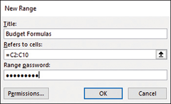
Use the New Range dialog box to name, specify, and password-protect a range.
If you want the password requirement to not apply to specific users or groups, click Permissions, and then in the Permissions dialog box, do the following:
Click Add, enter the name of a user or group, and then click OK to add the user or group to the Permissions dialog box.
Click the user or group, and then for the Edit range without a password permission, make sure the Allow check box is selected.
Click OK to return to the New Range dialog box.
In the New Range dialog box, click OK, reenter the password to confirm it, and then click OK. Excel adds the range to the Allow Users To Edit Ranges dialog box.

Your protected ranges appear in the Allow Users To Edit Ranges dialog box.
Repeat steps 2 through 7 to protect other ranges, and then click OK to close the dialog box and save your changes.
Important
The range password doesn’t go into effect until you activate worksheet protection.
To activate worksheet protection
Do either of the following to open the Protect Sheet dialog box:
On the Review tab, in the Protect group, click Protect Sheet.
If the Allow Users To Edit Ranges dialog box is open, click the Protect Sheet button in that dialog box.
In the Protect Sheet dialog box, do the following, and then click OK:
Select the Protect worksheet and contents of locked cells check box.
If you want, for added security, enter a password in the Password to unprotect sheet box. This means that no one can turn off the worksheet’s protection without first entering the password.
In the Allow all users of this worksheet to list, select the check box beside each action you want unauthorized users to be allowed to perform.

Use the Protect Sheet dialog box to activate your protection formatting or range passwords.
If you entered a password, reenter the password, and then click OK to continue working in the worksheet.
Protect workbook structure
When you protect a workbook’s structure, Excel takes the following actions:
Disables most of the worksheet-related commands on the ribbon. For example, on the Home tab, on the Format menu, the Rename Sheet and Move Or Copy Sheet commands are unavailable.
Disables most of the commands on the worksheet tab’s shortcut menu, including Insert, Delete, Rename, and Move or Copy.
Keeps the Scenario Manager from creating a summary report.
To protect the workbook structure
In the workbook you want to protect, on the Review tab, in the Protect group, click Protect Workbook to display the Protect Structure and Windows dialog box.

Use the Protect Structure and Windows dialog box to prevent changes to your workbook’s formatting and worksheet structure.
Enter an optional password in the Password text box, and then click OK.
Select the Structure check box.
If you specified a password, reenter the password to confirm, and then click OK.
Configure formula calculation options
Excel always calculates a formula when you confirm its entry, and the program normally recalculates existing formulas automatically whenever their data changes. This behavior is fine for small worksheets, but it can slow you down if you have a complex model that takes several seconds or even several minutes to recalculate. To turn off this automatic recalculation, Excel gives you two ways to get started:
You can use commands on the Calculation Options menu on the Formula tab.
You can use settings on the Formulas page of the Excel Options dialog box.
Either way, you’re presented with three calculation options:
Automatic This is the default calculation mode; it means that Excel recalculates formulas as soon as you enter them and as soon as the data for a formula changes.
Automatic except for data tables In this calculation mode, Excel recalculates all formulas automatically, except for those associated with data tables. This is a good choice if your worksheet includes one or more massive data tables that are slowing down the recalculation.
Manual Select this mode to force Excel not to recalculate any formulas until you either manually recalculate or save the workbook.
With manual calculation turned on, Calculate appears in the status bar whenever your worksheet data changes and your formula results need to be updated.
See Also
For more information about manually calculating parts of formulas, see “Evaluate formulas” in “Objective 3.5: Troubleshoot formulas.”
When you manually recalculate a workbook, note that Excel doesn’t necessarily recalculate every formula in the workbook. To minimize workbook recalculation, Excel builds a dependency tree that details not only the operands in each workbook formula (such as the functions it calls), but also any formulas used in cells referenced by each formula. A formula that relies on the results of calculations in another cell is said to be dependent on that cell. The dependency tree follows a formula’s chain of references until there are no more references left to check.
See Also
For more information about formula dependencies, see “Trace precedence and dependence” in “Objective 3.5: Troubleshoot formulas.”
Using the dependency tree, when you recalculate a workbook, Excel only updates formulas in this order:
Formulas that have changed or that have changed range names.
Formulas that include volatile functions. (A volatile function is one where its value changes each time you recalculate or reopen the worksheet or edit any cell on the worksheet; the RAND worksheet function is an example.)
Formulas that are dependent on other formulas that have changed, use range names that have changed, or use volatile functions.
When you manually recalculate a workbook, Excel updates every formula in the dependency tree. However, Excel might not update a particular formula if the dependency tree is incorrect or out of date (for whatever reason). Excel offers a manual workbook recalculation method that you can invoke to force Excel to rebuild its dependency tree.
You can also control various options for iterative calculations. These are calculations where you begin with a guess at the solution, plug that guess into the formula to get a new solution, plug that solution into the formula, and then keep repeating this procedure. Each time you plug a new solution into the formula it is called an iteration, so the entire process is called an iterative calculation. This type of calculation creates a circular reference, which is normally an error in Excel, so that’s why iterative calculations are turned off by default.
How does an iterative calculation know when to stop? If during the iterative process the change from one solution to the next becomes smaller than some predetermined value, the formula is said to have converged on the solution. Because the formula might not ever converge—or it might only converge after an unacceptably large number of iterations—you can also tell Excel to stop after a predetermined number of iterations.
To enable the management of iterative calculations, the Formulas tab in the Excel Options dialog box offers two controls:
Maximum Iterations This value is the number of iterations after which Excel must stop the calculation if it hasn’t yet converged to a solution. The default value is 100.
Maximum Change This value is the threshold that Excel uses to determine whether the iterative calculation has converged on a solution. If the change in the formula result from one iteration is less than this value, Excel considers the formula solved and stops the iteration. The default value is 0.001, but you can reduce this (for example, to 0.0001 or 0.00001) if you require a solution with more precision.
When performing an iterative calculation, Excel stops the calculation as soon as it hits the Maximum Iterations value or the Maximum Change value (whichever comes first).
To configure the formula calculation options
➜ On the Formulas tab, in the Calculation group, click Calculation Options, and then click Automatic, Automatic Except for Data Tables, or Manual.

On the Formulas tab, click Calculation Options to choose how you want Excel to calculate workbook formulas.
Or
Click File, then click Options.
In the Excel Options dialog box, on the Formulas page, in the Calculation Options section, under Workbook Calculation, select the option you want.
If you select the Manual option and want to run the calculation automatically when you save the file, select the Recalculate workbook before saving check box.

On the Formulas page of the Excel Options dialog box, select a Workbook Calculation option to tell Excel how to calculate workbook formulas.
Click OK.
To manually recalculate a single formula
Select the cell containing the formula.
Click in the formula bar, and then press Enter or click the Enter button.
To manually recalculate formulas in a selected cell range
Display the Replace tab of the Find and Replace dialog box.
Enter an equal sign (=) in both the Find What and Replace With boxes.
Click Replace All.
Tip
This procedure doesn’t actually change any formulas, but it forces Excel to recalculate each formula.
To manually recalculate formulas in only the active worksheet
➜ On the Formulas tab, click Calculate Sheet.
Or
➜ Press Shift+F9.
To manually recalculate changed formulas in every open workbook
➜ On the Formulas tab, in the Calculation group, click Calculate Now.
Or
➜ Press F9.
To manually recalculate every formula (changed or unchanged) in every open workbook
➜ Press Ctrl+Alt+F9.
To manually recalculate every formula (changed or unchanged) in every open workbook and rebuild the dependency tree
➜ Press Ctrl+Alt+Shift+F9.
Tip
Excel supports multithreaded calculation on computers with either multiple processors or processors with multiple cores. For each processor (or core), Excel sets up a thread (a separate process of execution). Excel can then use each available thread to process multiple calculations concurrently. For a worksheet with multiple, independent formulas, multithreaded calculation can dramatically speed up calculations. To verify that multithreaded calculation is turned on, display the Advanced page of the Excel Options dialog box and, in the Formulas section, ensure that the Enable Multi-Threaded Calculation check box is selected.
To enable and configure iterative calculations
Click File, click Options.
In the Excel Options dialog box, on the Formulas page, in the Calculation options section, select the Enable iterative calculation check box.
In the Maximum Iterations box, enter or select the number of iterations Excel can try before it must stop the calculation.
In the Maximum Change box, enter the numeric value that you want Excel to use as a threshold to determine whether the calculation has converged on a solution.

Use the Formulas page of the Excel Options dialog box to enable and configure iterative calculations.
Click OK.
Manage comments
When building a spreadsheet model, it is often useful to get feedback from other people. Feedback might include verification of some content, confirmation that a formula works as it should, suggestions for improving the layout, a critique of the overall model, or just general notes about the worksheet. If someone sends you a workbook and requests your feedback, you can place that feedback in a separate document such as an email message or a Word document. However, this means your feedback will lack context. You can work around this by specifying the cell or range you’re talking about, but it still means the owner of the workbook has to go back and forth between the documents.
A better way to provide worksheet feedback is to add that feedback directly to the worksheet itself. However, rather than typing text into a worksheet cell, you can instead add a comment, which is text that Excel associates with an individual cell but keeps separate from the worksheet itself. A comment is a review feature that starts a conversation about the cell’s contents because it enables other reviewers to read and respond to existing comments. A collection of one or more comments about a cell is called a thread. To close a particular comment thread and prevent further replies, you can resolve the thread. If you find that a comment thread is no longer required, you can delete it.
Important
Comment threads are a relatively new review feature in Excel. If you’re a longtime Excel user, do not confuse a comment thread that enables interaction between multiple users, with the original Excel style of comment, which was a single-user text annotation associated with a cell. The latter feature still exists in Excel but is now known as a note.
To start a new comment thread
Click the cell to which you want to add the comment thread.
On the Review tab, in the Comments group, click New Comment. Excel creates the comment and displays a pop-up window for typing the comment text.
Type your comment in the text box provided; then click Post or press Ctrl+Enter. Excel adds the comment and displays the comment marker in the top-right corner of the cell.

After you click New Comment, type your comment in the text box provided.
To navigate worksheet comments
➜ On the Review tab, in the Comments group, click Next Comment to display the next comment that appears in the worksheet.
➜ On the Review tab, in the Comments group, click Previous Comment to display the previous comment that appears in the worksheet.
➜ On the Review tab, in the Comments group, click Show Comments to open the Comments pane, which displays all the comments that appear in the worksheet. You can also click the Comments button that appears near the right edge of the ribbon.

The Comments pane displays all the comments added to the worksheet.
To edit a comment
➜ Move the mouse pointer over a cell that contains a comment (that is, a cell that displays a comment marker in the top-right corner), move the mouse pointer into the comment box, and then click Edit.
Or
➜ Display the Comments pane, click the comment you want to edit, and then click Edit.
To read a comment
➜ Move the mouse pointer over a cell that contains a comment (that is, a cell that displays a comment marker in the top-right corner).
➜ Display the Comments pane and view the comment in the list.
To respond to a comment
➜ Move the mouse pointer over a cell that contains a comment, click inside the Reply text box, type the response, and then click Post or press Ctrl+Enter.
➜ Display the Comments pane, locate the comment to which you want to reply, click inside the Reply text box, type the response, then click Post or press Ctrl+Enter.
To resolve a comment thread
➜ Move the mouse pointer over a cell that contains a comment, click the More Thread Options (...) button, and then click Resolve Thread.
➜ Display the Comments pane, locate the comment you want to resolve, click the More Thread Options (...) button, and then click Resolve Thread.
Tip
To reopen a cell’s comment thread for more replies and for editing, move the mouse pointer over the cell and then click Reopen Thread.
To delete a comment thread
➜ Move the mouse pointer over a cell that contains a comment, click the More Thread Options (...) button, and then click Delete Thread.
➜ Display the Comments pane, locate the comment you want to resolve, click the More Thread Options (...) button, and then click Delete Thread.
Tip
To delete a single comment reply rather than the entire comment thread, move the mouse pointer over a cell that contains a comment, move the mouse pointer over the reply you want to remove, and then click Delete.
Objective 1.2 practice tasks
The practice files for these tasks are located in the MOSExcelExpert2019Objective1 practice file folder. The folder also contains result files that you can use to check your work.
➤ Open the ExcelExpert_1-2a workbook and do the following:
❑ Unlock the cells in the range C3:C7.
❑ Activate worksheet protection. Do not enter a password. Do not allow users to select locked cells or to format cells.
❑ Ensure that users can modify the loan parameters in the range C3:C7 but cannot change anything else on the worksheet.
❑ Save the ExcelExpert_1-2a workbook.
❑ Open the ExcelExpert_1-2a_results workbook. Compare the two workbooks to check your work. Then close the open workbooks.
➤ Open the ExcelExpert_1-2b workbook and do the following:
❑ Unlock the cells in the range B2:B6.
❑ Protect the cells in the range B7:B8 with the password MOS123.
❑ Protect the worksheet with the same password.
❑ Save the ExcelExpert_1-2b workbook.
❑ Open the ExcelExpert_1-2b_results workbook. To unlock the range and sheet, use the password mos. Compare the two workbooks to check your work. Then close the open workbooks.
➤ In Excel, verify that formula calculations are set to automatic and iterative calculations are turned off.
➤ Open the ExcelExpert_1-2c workbook, dismiss the circular reference warning, and do the following:
❑ Change the formula calculation method to Manual and turn on iterative calculations.
❑ Select cell C6, which contains the circular reference formula, and manually calculate the formula result.
❑ Open the ExcelExpert_1-2c_results workbook. Compare the two workbooks to check your work.
❑ To preserve the initial circular reference, close the ExcelExpert_1-2c workbook without saving it.
➤ Open the ExcelExpert_1-2d workbook and do the following:
❑ Add a comment to any cell that does not already display a comment marker.
❑ Use the Next Comment and Previous Comment commands to navigate the worksheet comments.
❑ Navigate to the comment you added and then edit that comment.
❑ Add a reply to the comment in cell B3.
❑ Resolve the comment thread you added.
❑ Delete the comment thread you added.
❑ Close the ExcelExpert_1-2d workbook without saving it.
Objective 1.3: Use and configure language options
Configure authoring and display languages
You can change the language that Excel uses for authoring and for the display (the ribbon, buttons, tabs, and other interface features). You are free to apply a different language for authoring and display, depending on the languages available in the version of Windows or Office that you are using and the Windows language packs that you have installed. You can install additional languages from the Language page of the Excel Options dialog box. If you have multiple languages installed, you can tell Excel which language you prefer to use. You can also set a language priority order, which tells Excel which languages to use, in order, if the display language is not available in your default language.
To add an authoring language
Click File, then click Options.
In the Excel Options dialog box, on the Language page, click Add a Language.
Use the Add an authoring language list to select the language you want to install.
Click Add. Excel adds the language to the Office Authoring Languages and Proofing list.
Tip
For your new language, if you see Proofing Available, then you need to install the associated language pack from the Office.com website. Click the Proofing Available link to display the language pack page, click Download, and then run the downloaded file to install the language pack.

When you add a language, Excel displays it in the Office Authoring Languages and Proofing list.
To change the display language priority order
➜ In the Excel Options dialog box, on the Language page, click a language in the Office Display Language list, and then use the Move Up (higher priority) and Move Down (lower priority) buttons to position the language in the list.
Tip
To add more display languages, click the Install Additional Display Languages from Office.com link, which opens a page that enables you to download a language pack accessory for Office.

Use the Move Up and Move Down buttons to set a language’s priority.
To set the preferred languages
➜ In the Excel Options dialog box, on the Language page, click a language in the Office Authoring Languages and Proofing list, and then click the Set Preferred button that appears to the right of the list.
➜ In the Excel Options dialog box, on the Language page, click a language in the Office Display Language list, and then click the Set Preferred button that appears to the right of the list.
To remove an authoring language
➜ In the Excel Options dialog box, on the Language page, click a language in the Office Authoring Languages and Proofing list, click Remove, and then restart Excel to put the change into effect.
Use language-specific features
With your languages configured, you can now switch from one language to another within Excel. For example, you can switch to another language to add or edit Excel data and you can set another language as Excel’s default proofing dictionary.
Another language tool that comes in handy when you are working with other languages is the Translate command on the Review tab. This command opens the Translator task pane, which includes From and To boxes, where From shows the original text and To shows the language to which you want the original text translated. Translator attempts to recognize the original language, but if it gets the language wrong, you can select the correct language from a list. You can also select the language to which you want the original text translated.
To add and edit text in another language
➜ In the Excel Options dialog box, on the Language page, click a language in the Office Authoring Languages and Proofing list, and then click the Set Preferred button that appears to the right of the list.
To proof in another language
Click File, then click Options.
In the Excel Options dialog box, on the Proofing page, use the Dictionary language list to select the language you want to use.

Use the Dictionary Language list to select a proofing language.
To translate cell text
Select the cell that contains the text you want to translate.
On the Review tab, click the Translate button. The Translator pane appears.

Use the Translator pane to translate text form one language to another.
If Translator did not select the correct original language, use the From list to select the language.
Use the To list to select the language to which you want the original text translated.
Objective 1.3 practice tasks
The practice files for these tasks are located in the MOSExcelExpert2019Objective1 practice file folder.
➤ Open the ExcelExpert_1-3a workbook and do the following:
❑ Add the authoring language French (Canada).
❑ Add the language French as a display language.
❑ In the Office Display Language list, select French, and move its priority up and then down.
❑ In the Office Authoring Languages and Proofing list, select French (Canada), set it as the preferred language, and then return the preferred to your original language.
❑ In the Office Authoring Languages and Proofing list, select French (Canada), remove it, restart Excel, and then reopen the ExcelExpert_1-3a workbook.
❑ Select cell A1 and then run the Translate command to translate the French text into English.
❑ Close the ExcelExpert_1-3a workbook.