
Objective group 3
Create advanced formulas and macros
Objective 3.1: Perform logical operations in formulas
Insert functions into a formula
Formulas that combine operators with basic operands such as numeric and string values are the mainstay of any Excel spreadsheet. But to get the most benefit from the spreadsheet model, you need to expand your formula repertoire to include worksheet functions. Excel includes dozens of these functions, and they’re essential to making your worksheet easier to work with and more powerful.
To insert a function into a formula
Enter your formula up to the point where you want to insert the function.
On the Formulas tab, in the Function Library group, click the category that contains the function you want to use. Then on the category menu, click the function.
In the Function Arguments dialog box, enter the function arguments, then click OK.
Perform logical operations by using the IF, AND, OR, and NOT functions
In the computer world, we very loosely define something as intelligent if it can perform tests on its environment and act in accordance with the results of those tests. However, a computer is a binary machine, so “acting in accordance with the results of a test” means that it can do only one of two things. Even with this limited range of options, you can still bring a great deal of intelligence to your worksheets. Your formulas will be able to test the values in cells and ranges and then return results based on those tests. This is all done with the logical functions in Excel, which are designed to create decision-making formulas.
The following table describes the most common logical functions.
Function |
Description |
IF(logical_test, value_if_true[, value_if_false]) |
Performs a logical test and returns a value based on the result |
AND(logical1[, logical2,...]) |
Returns TRUE if all the arguments are true |
OR(logical1[, logical2,...]) |
Returns TRUE if any argument is true |
NOT(logical) |
Reverses the logical value of the argument |
You use the IF function to test some condition and then return a value based on the result of that test. This is the simplest version of the IF function:
IF(logical_test, value_if_true)
The logical_test argument is a logical expression—that is, an expression that returns TRUE or FALSE (or their equivalent numeric values: 0 for FALSE and any other number for TRUE); the value_if_true argument is the value returned by the function if logical_test evaluates to TRUE.
A logical expression compares two or more numbers, text strings, cell contents, or function results. If the expression is true, it’s given the logical value TRUE (which is equivalent to any nonzero value); if the expression is false, it’s given the logical value FALSE (which is equivalent to zero). The following table summarizes the comparison operators you can use in logical expressions.
Operator |
Name |
Example |
Result |
= |
Equal to |
=10=5 |
FALSE |
> |
Greater than |
=10>5 |
TRUE |
< |
Less than |
=10<5 |
FALSE |
>= |
Greater than or equal to |
="a">="b" |
FALSE |
<= |
Less than or equal to |
="a"<="b" |
TRUE |
<> |
Not equal to |
="a"<>"b" |
TRUE |
For example, suppose cell B2 contains a sales rep’s total sales and you want to give the rep a 10-percent bonus if those sales are greater than $100,000. Here’s a formula that does that:
=IF(B2 > 100000, B2 * 0.1)
The logical expression B1 > 100000 is used as the test. Assume that you add this formula to cell C2. If the logical expression proves to be true (that is, if the value in cell B2 is greater than 100,000), the function returns the value B2 * 0.1—that is, 10 percent of the number in B2—and that’s the value you see in cell C2.

A formula that uses the IF function to return a bonus for reps with sales greater than 100,000.
When the IF function test returns FALSE (that is, the value in column B is less than or equal to 100,000), the function returns FALSE as its result. That’s not inherently bad, but the worksheet would look tidier (and, hence, be more useful) if the formula returned, for instance, the value 0 instead.
To do this, you need to use the full IF function syntax:
IF(logical_test, value_if_true, value_if_false)
The extra value_if_false argument is the value returned by the function if logical_test evaluates to FALSE. Here’s a modification of the sales rep bonus calculation that takes a FALSE result into account:
=IF(B2 > 100000, B2 * 0.1, 0)
It’s often necessary to perform an action if and only if two conditions are true. For example, you might want to pay a salesperson a bonus if and only if dollar sales exceed a certain amount and unit sales also exceed some minimum value. If the dollar sales, the unit sales, or both fall below the minimum, no bonus is paid. In Boolean logic, this is called an And condition because one expression and another must be true for a positive result.
In Excel, And conditions are handled by the AND logical function:
AND(logical1[, logical2,...])
Here, logical1 and logical2 arguments are the logical conditions to test. (The ellipsis means that you can enter as many conditions as you need.) The AND result is calculated as follows:
If all the arguments return TRUE (or any nonzero number), AND returns TRUE.
If one or more of the arguments return FALSE (or 0), AND returns FALSE.
Consider a formula that uses AND to check whether a sales rep’s sales total is greater than $100,000 and units total is greater than 10,000. That formula could look like this:
=AND(B2 > 100000, C2 > 10000)

A formula that uses the AND function to test whether the values in columns B and C exceed a specified minimum.
In many worksheet models, you need to take an action if one thing or another is true. For example, you might want to pay a salesperson a bonus if she exceeds the dollar sales budget or if she exceeds the unit sales budget. In Boolean logic, this is called an Or condition.
In Excel, Or conditions are handled by the OR function:
OR(logical1[, logical2,...])
Here, logical1 and logical2 arguments are the logical conditions to test. (The ellipsis means that you can enter as many conditions as you need.) The OR result is calculated as follows:
If one or more of the arguments return TRUE (or any nonzero number), OR returns TRUE.
If all of the arguments return FALSE (or 0), OR returns FALSE.
Consider the following formula, which uses OR to check whether a sales rep’s sales total is greater than $100,000 or the units total is greater than 10,000:
=OR(B2 > 100000, C2 > 10000)

A formula that uses the OR function to test whether the values in columns B or C exceed a specified minimum.
You sometimes need to return the opposite of a logical expression. For example, you might want to set up a worksheet that looks for the sales reps who did not make their sales quota and then flag those reps for further training. If you have a worksheet that already returns a TRUE or FALSE value based on whether a sales rep meets his quota, flagging whether the sales rep needs more training is a matter of returning the opposite value: if a sales rep meets her quota (TRUE), she doesn’t need training (FALSE); if a sales rep doesn’t meet his quota (FALSE), he does need training (TRUE).
In Excel, you return the opposite of a logical expression by using the NOT function:
NOT(logical)
Here, the logical argument is the logical condition to test. The NOT result is calculated as follows:
If logical is TRUE (or any nonzero number), NOT returns FALSE.
If logical is FALSE (or 0), NOT returns TRUE.
The following formula uses NOT in the Training Required? column (E) to return the opposite of the logical value in the Bonus column (D):
=NOT(D2)

A formula that uses the NOT function to return the opposite of the logical values in column D.
To insert a logical function into a formula
➜ On the Formulas tab, in the Function Library group, click Logical, click one of the functions in the list (such as IF, AND, OR, or NOT), and then enter the arguments, if any, as described earlier in this topic.
Perform logical operations by using nested functions
You can create sophisticated logical tests by combining one or more logical functions within a single expression. In particular, you can create complex expressions by including one logical function within another. This is called nesting, and the inner function is called a nested function.
A good time to use nested IF functions arises when you need to calculate a tiered payment or charge. That is, if a certain value is X, you want one result; if the value is Y, you want a second result; and if the value is Z, you want a third result. For example, suppose you want to calculate tiered bonuses for a sales team as follows:
If the salesperson did not meet the sales target, no bonus is given.
If the salesperson exceeded the sales target by less than 10 percent, a bonus of $1,000 is awarded.
If the salesperson exceeded the sales target by 10 percent or more, a bonus of $5,000 is awarded.
Assuming that cell D2 contains the percentage that each salesperson’s actual sales were above or below her target sales, here’s a formula that handles these rules:
=IF(D2 < 0, "", IF(D2 < 0.1, 1000, 5000))

A formula that uses nested IF functions to calculate a tiered bonus.
To nest logical functions
Insert the first logical function into your formula.
Enter the function arguments as described earlier in this topic, including the logical function you want to nest as one of the arguments.
Perform multiple logical tests with the IFS function
Nesting one IF function inside another is a handy way to perform a couple of logical tests, but the method quickly becomes unwieldly and difficult to decipher when the nesting goes three or more IF functions deep. If your data analysis requires more than two logical tests, you can make your worksheet model easier to read by turning to the IFS function:
IFS(logical_test1, value_if_true1, [logical_test2, value_if_true2,…])
The IFS function consists of a series of logical tests, each of which has an associated return value. IFS performs each logical test in turn, and when it comes across the first logical test to return TRUE, it returns that logical test’s associated value.
For example, here’s how you’d use IFS to calculate the tiered bonuses that I introduced in the previous section:
=IFS(D2 < 0, 0, D2 < 0.1, 1000, D2 >= 0.1, 5000)

A formula that uses the IFS function to calculate a tiered bonus.
Perform logical operations with criteria
You use the SUM, AVERAGE, and COUNT functions in Excel to return the total value, the mean value, and the number of values, respectively, within a specified range. These functions operate over the entire range, but it’s often the case that you want the sum, the average, or the count of only those cells that meet some criterion. For example, you might want the total sales for just the customers from the United States. Even more sophisticated calculations are possible when you use multiple criteria. For example, you might want the total sales for those customers who are from the United States and who are based in Oregon.
These seem like they would require complex combinations of the IF, AND, and OR functions nested within the SUM, AVERAGE, or COUNT function. Fortunately, Excel includes three summary functions that you can use to specify multiple criteria without complex nesting: SUMIF, AVERAGEIF, and COUNTIF. In each case, the “IF” part of the function name implies that an IF function is built into each function, without being explicitly invoked.
The SUMIF function is similar to SUM, except that it sums only those cells in a range that meet a specified condition:
SUMIF(range, criteria[, sum_range])
Here, the range argument is the range of cells to use for the criteria; the criteria argument is the criteria, entered as text, that Excel applies to range to determine which cells to sum; sum_range is an optional argument that specifies the range from which the sum values are taken. Excel sums only those cells in sum_range that correspond to the cells in range and meet the criteria. If you omit sum_range, Excel uses range for the sum.
For the criteria argument, you generally use the following format:
"operator value"
Here, you replace operator with a comparison operator such as equal to (=) or greater than (>), and you replace value with a comparison value. Many Excel functions also support text-only criteria arguments that optionally use one or more wildcard characters: * to match any number of characters and ? to match any single character.
For example, the following formula sums only those values in the range B3:B21 that are greater than 100000:
=SUMIF(B3:B21, "> 100000")

A formula that uses the SUMIF function.
The COUNTIF function counts the number of cells in a range that meet a single condition:
COUNTIF(range, criteria)
Here, replace range with the range of cells to use for the count; replace criteria with the criteria, entered as text, that Excel applies to range to determine which cells to count.
For example, you can use the following formula to count the number of cells in the range D3:D21 that are greater than or equal to 0.1:
=COUNTIF(D3:D21, ">= 0.1")
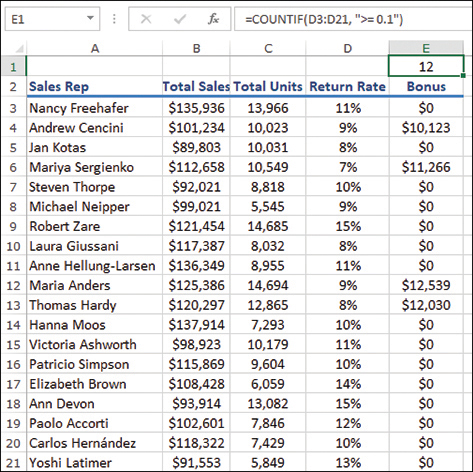
A formula that uses the COUNTIF function.
The AVERAGEIF function calculates the average of a range set for those items that meet a specified condition:
AVERAGEIF(range, criteria[, average_range])
Here, the range argument is the range of cells to use for the criteria; the criteria argument is the criteria, entered as text, that Excel applies to range to determine which cells to average; average_range is an optional argument that specifies the range from which the average values are taken. Excel averages only those cells in average_range that correspond to the cells in range and meet the criteria. If you omit average_range, Excel uses range for the average.
For example, the following formula averages only those values in the range D3:D21 that correspond to those values in the range C3:C21 that are greater than or equal to 10,000:
=AVERAGEIF(C2:C21, "> 10000", D3:21)

A formula that uses the AVERAGEIF function.
To insert a SUMIF function into a formula
➜ On the Formulas tab, in the Function Library group, click Math & Trig, click SUMIF, and then enter the arguments, as described earlier in this topic.
To insert an AVERAGEIF or COUNTIF function into a formula
➜ On the Formulas tab, in the Function Library group, click More Functions, click Statistical, click AVERAGEIF or COUNTIF, and then enter the arguments, as described earlier in this topic.
Perform logical operations with multiple ranges and criteria
The SUMIF, COUNTIF, and AVERAGEIF functions that I describe in the previous section replace simple nested functions with a single condition. However, there are many situations in which your logical formula requires multiple criteria applied to multiple ranges. To handle these situations, Excel includes five summary functions that you can use to specify multiple criteria: SUMIFS, AVERAGEIFS, COUNTIFS, MAXIFS, and MINIFS. In each case, the “IFS” part of the function name implies that multiple IF functions are built into each function, without being explicitly invoked.
The SUMIFS function sums cells in a range that correspond to those cells in one or more ranges that meet one or more criteria:
SUMIFS(sum_range, range1, criteria1[, range2, criteria2, ...])
The sum_range argument is the range from which the sum values are taken. Excel sums only those cells in sum_range that correspond to the cells that meet the criteria. The range1 argument is the first range of cells to use for the sum criteria, and the criteria1 argument is the first criterion, entered as text, that determines which cells to sum. Excel applies the criterion to range1. You can enter up to 127 range/criterion pairs.
Consider the following SUMIFS function example. In this model, SUMIFS is used to calculate the total bonuses (range E3:E21) just for those sales reps whose total units (range C3:C21) are greater than 10,000:
=SUMIFS(E3:E21, C3:C21, " > 10000")

A formula that uses SUMIFS to apply a criterion to a sum.
The AVERAGEIFS function averages cells in a range that correspond to those cells in one or more ranges that meet one or more criteria:
AVERAGEIFS(average_range, range1, criteria1[, range2, criteria2, ...])
The average_range argument is the range from which the average values are taken. Excel averages only those cells in average_range that correspond to the cells that meet the criteria. The range1 argument is the first range of cells to use for the average criteria, and the criteria1 argument is the first criterion, entered as text, that determines which cells to average. Excel applies the criterion to range1. You can enter up to 127 range/criterion pairs.
In the following example, AVERAGEIFS is used to calculate the average sales (range B3:B21) just for those sales reps whose total units (C3:C21) are greater than 10,000 and whose return rate (D3:D21) is less than 10 percent:
=AVERAGEIFS(B3:B21, C3:C21, " > 10000", D3:D21, " < 0.1")

A formula that uses AVERAGEIFS to apply multiple criteria to an average.
The COUNTIFS function counts the number of cells in one or more ranges that meet one or more criteria:
COUNTIFS(range1, criteria1[, range2, criteria2, ...])
The range1 argument is the first range of cells to use for the count, and the criteria1 argument is the first criterion, entered as text, that determines which cells to count. Excel applies the criterion to range1. You can enter up to 127 range/criterion pairs.
In the following example, COUNTIFS is used to count the number of sales reps whose dollar sales (range B3:B21) are greater than $100,000, whose unit sales (C3:C21) are greater than 10,000, and whose return rate (D3:D21) is less than 10 percent:
=COUNTIFS(B3:B21, " > 100000", C3:C21, " > 10000", D3:D21, " < 0.1")

A formula that uses COUNTIFS to apply multiple criteria to a count.
The MAXIFS function returns the maximum value from a range that corresponds to those cells in one or more ranges that meet one or more criteria:
MAXIFS(max_range, range1, criteria1[, range2, criteria2, ...])
The max_range argument is the range from which the maximum value is taken. Excel looks for the maximum only in those cells in max_range that correspond to the cells that meet the criteria. The range1 argument is the first range of cells to use for the maximum criteria, and the criteria1 argument is the first criterion, entered as text, that determines which cells to include. Excel applies the criterion to range1. You can enter up to 127 range/criterion pairs.
Consider the following MAXIFS function example. In this model, MAXIFS is used to calculate the maximum return rate (from the range D3:D21) just for those sales reps whose total sales (range B3:B21) are greater than $100,000 and whose total units (range C3:C21) are greater than 10,000:
=MAXIFS(D3:D21, B3:B21, "> 100000", C3:C21, " > 10000")

A formula that uses MAXIFS to apply a criterion to a maximum.
The MINIFS function returns the minimum value from a range that corresponds to those cells in one or more ranges that meet one or more criteria:
MINIFS(min_range, range1, criteria1[, range2, criteria2, ...])
The min_range argument is the range from which the minimum value is taken. Excel looks for the minimum only in those cells in min_range that correspond to the cells that meet the criteria. The range1 argument is the first range of cells to use for the minimum criteria, and the criteria1 argument is the first criterion, entered as text, that determines which cells to include. Excel applies the criterion to range1. You can enter up to 127 range/criterion pairs.
Consider the following MINIFS function example. In this model, MINIFS is used to calculate the minimum units (from the range C3:C21) just for those sales reps whose total sales (range B3:B21) are greater than $100,000 and whose return rate (range D3:D21) are less than 10 percent:
=MINIFS(C3:C21, B3:B21, " > 100000", D3:D21, "< 0.1")

A formula that uses MINIFS to apply a criterion to a minimum.
To insert a SUMIFS function into a formula
➜ On the Formulas tab, in the Function Library group, click Math & Trig, click SUMIFS, and then enter the arguments, as described earlier in this topic.
To insert an AVERAGEIFS, COUNTIFS, MAXIFS, or MINIFS function into a formula
➜ On the Formulas tab, in the Function Library group, click More Functions, click Statistical, click the function—AVERAGEIFS, COUNTIFS, MAXIFS, or MINIFS,—and then enter the arguments, as described earlier in this topic.
Apply multiple exact-match criteria to a value
The IFS function that I describe earlier in this objective enables you to create sophisticated criteria using comparison operators such as less than (<) and greater than or equal to (>=). However, it’s often the case that your comparisons require only exact matches using the equal operator (=). In such cases, it is often easier to use the SWITCH function rather than IFS.
The SWITCH function evaluates an expression, compares the result to a list of values that you supply, and then returns a value that corresponds to the first match that Excel finds:
SWITCH(expression, value_to_match1, value_to_return1[, value_to_match2, value_to_return2, ..., value_if_no_match])
SWITCH first evaluates expression. SWITCH then compares that result to each value_to_match argument; when SWITCH comes across the first match, it returns the corresponding value_to_return; if no match is found, SWITCH returns the value_if_no_match argument. You can enter up to 126 match/return value pairs.
For example, given a date, the MONTH function returns a number between 1 (for January) and 12 (for December). For a date in cell A2, you can use the following SWITCH formula to return the date’s month name based on the results of the MONTH(A2) expression:
==SWITCH(MONTH(A2), 1, "January", 2, "February", 3, "March", 4, "April", 5, "May", 6, "June", 7, "July", 8, "August", 9, "September", 10, "October", 11, "November", 12, "December", "No matching month!")

A formula that uses SWITCH to apply multiple exact-match criteria to an expression.
To insert a SWITCH function into a formula
➜ On the Formulas tab, in the Function Library group, click Logical, click SWITCH, and then enter the arguments, as described earlier in this topic.
Objective 3.1 practice tasks
The practice file for these tasks is located in the MOSExcelExpert2019Objective3 practice file folder. The folder also contains a result file that you can use to check your work.
➤ Open the ExcelExpert_3-1 workbook and do the following:
❑ On the Gross Margin worksheet, add formulas to the Gross Margin field (H7:H14) that calculate the gross margin by subtracting Cost from Retail and then dividing by Cost. To avoid #DIV/0! (division by 0) errors, wrap the calculation inside an IF function that returns the gross margin if Cost is not 0, or the message Cost is 0! otherwise.
❑ On the Inventory worksheet, populate the Reorder Now? column with formulas that use nested logical functions to determine whether a product should be reordered based on two conditions: The Qty Available is less than or equal to the Reorder Level, and the Qty on Order is 0. Each function should return “Yes” if a reorder is required, and nothing otherwise.
❑ On the Inventory worksheet, create a formula in cell K1 that uses the SUMIF function to sum the Value range for products with a non-zero Qty Available value.
❑ On the Inventory worksheet, create a formula in cell K2 that uses the SUMIFS function to sum the Qty On Hand range for products with a Product Name value that includes Soup and a Qty On Hold value of zero. (Hint: To match cells that include some text, surround that text with the * wildcard character.)
❑ On the Parts worksheet, create a formula in cell F16 that uses the AVERAGEIF function to calculate the average of the Gross Margin values for the parts that cost less than $10. Use structured table references in your formula (the table name is Parts).
❑ On the Customers worksheet, create a formula in cell L1 that uses the COUNTIFS function to return the number of customers with the Country value United States and the Region value OR (the abbreviation for Oregon, not the OR function).
❑ On the Orders worksheet, populate the Weekday column with formulas that use the SWITCH function to return the weekday of each date in the Date column.
➤ Save the workbook.
➤ Open the ExcelExpert_3-1_results workbook. Compare the two workbooks to check your work, and then close the open workbooks.
Objective 3.2: Look up data by using functions
The table—more properly referred to as a lookup table—is the key to performing lookup operations in Excel. The most straightforward lookup table structure is one that consists of two columns (or two rows):
Lookup column This column contains the values that you look up. For example, if you were constructing a lookup table for a dictionary, this column would contain the words.
Data column This column contains the data associated with each lookup value. In the dictionary example, this column would contain the definitions.
In most lookup operations, you supply a value that the function locates in the designated lookup column. It then retrieves the corresponding value in the data column.
The lookup table theme has many variations. The lookup table can be one of these:
A single column or row In this case, the lookup operation consists of finding the nth value in the column.
A range with multiple data columns For instance, in the dictionary example, you might have a second column for each word’s part of speech (noun or verb, for example), and perhaps a third column for its pronunciation. In this case, the lookup operation must also specify which of the data columns contains the value required.
An array In this case, the table doesn’t exist on a worksheet but is either an array of literal values or the result of a function that returns an array. The lookup operation finds a particular position within the array and returns the data value at that position.
The VLOOKUP function works by looking in the first column of a table for the value you specify. (The V in VLOOKUP stands for vertical.) It then looks across to the column that you specify and returns whatever value it finds there.
Here’s the full syntax for VLOOKUP:
VLOOKUP(lookup_value, table_array, col_index_num[, range_lookup])
The following table describes the VLOOKUP function arguments.
Argument |
Description |
lookup_value |
The value you want to find in the first column of table_array. You can enter a number, string, or reference. |
table_array |
The cell range or named table to use for the lookup. |
col_index_num |
The column number in table_array that contains the data you want the formula to return (the first column—that is, the lookup column—is 1, the second column is 2, and so on). |
range_lookup |
A Boolean value that determines how Excel searches for lookup_value in the first column. If FALSE, VLOOKUP returns the first exact match for lookup_value. If TRUE (the default), if no exact match is found, the function returns the largest value that is less than lookup_value. |
Here are some notes to keep in mind when you work with VLOOKUP:
If range_lookup is TRUE or omitted, you must sort the values in the first column in ascending order.
If the first column of the table is text, you can use the standard wildcard characters in the lookup_value argument (use ? to substitute for individual characters; use * to substitute for multiple characters).
If lookup_value is less than any value in the lookup column, VLOOKUP returns the #N/A error value.
If VLOOKUP doesn’t find a match in the lookup column, it returns #N/A.
If col_index_num is less than 1, VLOOKUP returns #VALUE!; if col_index_num is greater than the number of columns in table_array, VLOOKUP returns #REF!.
As an example, assume that a worksheet uses a VLOOKUP formula in cell B4 to take the account number entered in cell B2, locate the exact match in the first column of the range D3:E15, and return the account name from the second column in that range. The formula would look like this:
=VLOOKUP(B2, D3:E15, 2, FALSE)
The HLOOKUP function is similar to VLOOKUP except that it searches for the lookup value in the first row of a table. (The H in HLOOKUP stands for horizontal.) If successful, this function then looks down to the specified row and returns the value it finds there. Here’s the syntax for HLOOKUP:
HLOOKUP(lookup_value, table_array, row_index_num[, range_lookup])

A formula that uses VLOOKUP to look up an account name given an account number.
The following table describes the HLOOKUP function arguments.
Argument |
Description |
lookup_value |
The value you want to find in the first row of table_array. You can enter a number, string, or reference. |
table_array |
The cell range or named table to use for the lookup. |
row_index_num |
The row number in the table that contains the data you want the formula to return (the first row—that is, the lookup row—is 1, the second row is 2, and so on). |
range_lookup |
A Boolean value that determines how Excel searches for lookup_value in the first row. If FALSE, HLOOKUP returns the first exact match for lookup_value. If TRUE (the default), if no exact match is found, the function returns the largest value that is less than lookup_value. |
As an example, assume that a worksheet uses an HLOOKUP formula in cell C10 to take the month entered in cell C9, locate the exact match in the first row of the range C1:N7, and return the value from the TOTAL row (the seventh row in that range).
The formula would look like this:
=HLOOKUP(C9, C1:N7, 7, FALSE)

A formula that uses HLOOKUP to look up a monthly expenses total given a month name.
The basic lookup procedure—finding a value in a column or row and then returning an offset value—will satisfy most of your needs. However, a few operations require a more sophisticated approach that makes use of two more lookup functions: MATCH and INDEX.
The MATCH function looks through a row or column of cells for a value. If MATCH finds that value, it returns the relative position of the match in the row or column. Here’s the syntax:
MATCH(lookup_value, lookup_array[, match_type])
The following table describes the MATCH function arguments.
Argument |
Description |
lookup_value |
The value you want to find. You can use a number, string, reference, or logical value. |
lookup_array |
The row or column of cells you want to use for the lookup. |
match_type |
How you want Excel to match the lookup_value with the entries in the lookup_array. You have three choices:
|
Normally, you don’t use the MATCH function by itself; you combine it with the INDEX function. INDEX returns the value of a cell at the intersection of a row and column inside a reference. Here’s the syntax for INDEX:
INDEX(reference, row_num[, column_num][, area_num])
The following table describes the INDEX function arguments.
Argument |
Description |
reference |
A reference to one or more cell ranges. |
row_num |
The number of the row in reference from which to return a value. |
column_num |
The number of the column in reference from which to return a value. You can omit column_num if reference is a single column. |
area_num |
If you entered more than one range for reference, area_num is the range you want to use. The first range you entered is 1 (this is the default), the second is 2, and so on. |
The idea is that you use MATCH to get row_num and/or column_num (depending on how your table is laid out) and then use INDEX to return the value you need.
For example, consider a worksheet that uses a MATCH and INDEX formula in cell B2 to take the part number entered in cell B1, locate the match in the range H6:H13, and return the quantity from the range C6:C13.
The formula would look like this:
=INDEX(C6:C13, MATCH(B1, H6:H13, 0))

A formula that uses MATCH and INDEX to look up a quantity given a part number.
To insert a VLOOKUP or an HLOOKUP function into a formula
➜ On the Formulas tab, in the Function Library group, click Lookup & Reference, click VLOOKUP or HLOOKUP, and then enter the arguments, as described earlier in this topic.
To insert the MATCH and INDEX functions into a formula
On the Formulas tab, in the Function Library group, click Lookup & Reference, and then click INDEX.
In the Select Arguments dialog box, click reference,row_num,column_num,area_num, then click OK.
In the Function Arguments dialog box, enter the INDEX function arguments, including a MATCH function for the row_num and/or column_num arguments, and then click OK.
Objective 3.2 practice tasks
The practice file for these tasks is located in the MOSExcelExpert2019Objective3 practice file folder. The folder also contains a result file that you can use to check your work.
➤ Open the ExcelExpert_3-2 workbook and do the following:
❑ On the Tax Rate worksheet, add a formula to cell B18 that uses the tax table in the range C9:F15 to look up the income entered in cell B17 and return the applicable tax rate.
❑ On the Discount Schedule worksheet, create formulas in the range D3:D10 that use the discount schedule in the range B13:G14 to look up the units ordered from the range A3:A10 and return the applicable discount percentage.
❑ On the Parts worksheet, add a formula to cell B3 that uses the range A7:H14 to look up the part number entered in cell B1 and then return the corresponding value from the field entered in cell B2.
➤ Save the workbook.
➤ Open the ExcelExpert_3-2_results workbook. Compare the two workbooks to check your work, and then close the open workbooks.
Objective 3.3: Apply advanced date and time functions
You can use the date and time functions in Excel to convert dates and times to serial numbers and perform operations on those numbers. This capability is useful for such things as accounts receivable aging, project scheduling, time-management applications, and much more.
Excel uses serial numbers to represent specific dates and times. To get a date serial number, Excel uses December 31, 1899, as an arbitrary starting point and then counts the number of days that have passed since then. For example, the date serial number for January 1, 1900, is 1; for January 2, 1900, it’s 2; for June 6, 1944 its 16229, and so on.
To get a time serial number, Excel expresses time as a decimal fraction of the 24-hour day to return a number between 0 and 1. The starting point, midnight, is given the value 0, so noon—halfway through the day—has a serial number of 0.5, and 5:00 PM has a serial number of 0.70833. You can combine the two types of serial numbers. For example, 44196.5 represents noon on December 31, 2019.
The advantage of using serial numbers in this way is that it makes calculations involving dates and times very easy. A date or time is really just a number, so any mathematical operation you can perform on a number can also be performed on a date. This is invaluable for worksheets that track delivery times, monitor accounts receivable or accounts payable aging, and calculate invoice discount dates, for example.
Reference the date and time by using the NOW and TODAY functions
If you need a date for an expression operand or a function argument, you can enter it by hand if you have a specific date in mind. Much of the time, however, you need more flexibility, such as always entering the current date or time.
When you need to use the current date in a formula, a function, or an expression, use the TODAY function, which doesn’t take any arguments. This function returns the serial number of the current date, with midnight as the assumed time. For example, on November 1, 2019, the TODAY function returns the serial number 43770.0.

The TODAY function returns the current date serial number in the date format of the cell.
Note that TODAY is a dynamic function that doesn’t always return the same value. Each time you edit the formula, enter another formula, recalculate the worksheet, or reopen the workbook, TODAY updates its value to return the current system date.
When you need to use the current time in a formula, a function, or an expression, use the NOW function, which doesn’t take any arguments. This function returns the serial number of the current time, with the current date as the assumed date. For example, at 11:24 AM on November 1, 2019, the NOW function returns the serial number 43770.47549.

The NOW function returns the current date and time serial number in the date/time format of the cell.
If you want only the time component of the serial number, subtract TODAY from NOW:
=NOW - TODAY
Just like the TODAY function, NOW is a dynamic function that doesn’t keep its initial value (that is, the time at which you entered the function). Each time you edit the formula, enter another formula, recalculate the worksheet, or reopen the workbook, NOW updates its value to return the current system time.
To insert the TODAY or NOW function in a formula
➜ On the Formulas tab, in the Function Library group, click Date & Time, then click TODAY or NOW.
Serialize numbers by using date and time functions
The date functions in Excel work with or return date serial numbers. You can also work in the opposite direction by taking numbers that represent a specified year, month, and day, and serialize them into a valid Excel date. When you have a date serial number, you can use more Excel date functions to manipulate and perform calculations with those dates.
Similarly, the time functions work with or return time serial numbers, but you can also work in the opposite direction by taking numbers that represent a specified hour, minute, and second, and serialize them into a valid Excel time. When you have a time serial number, you can use other Excel time functions to manipulate and perform calculations with those times.
A date consists of three components: the year, month, and day. It often happens that a worksheet generates one or more of these components, and you need some way of building a proper date out of them. You can do that by using the DATE function:
DATE(year, month, day)
The following table describes the DATE function arguments.
Argument |
Description |
year |
The year component of the date (a number from 1900 through 9999) |
month |
The month component of the date (a number from 1 through 12) |
day |
The day component of the date (a number from 1 through 31) |
Important
Different versions of Excel and even different functions within the current version of Excel interpret two-digit years differently. For example, a year entered as 30 might be interpreted as either 1930 or 2030. To avoid problems, always use a four-digit value when entering the year component of any date.
For example, the expression DATE(2020, 12, 25) returns Christmas Day in 2020.
Note, too, that DATE adjusts for wrong month and day values. For example, the expression DATE(2020, 12, 32) returns January 1, 2021. Here, DATE adds the extra day (there are 31 days in December) to return the date of the next day.
The three components of a date—year, month, and day—can also be extracted individually from a specified date. This might not seem all that interesting at first, but many useful techniques arise out of working with a date’s component parts. You can extract a date’s components by using the YEAR, MONTH, and DAY functions:
YEAR(serial_number) MONTH(serial_number) DAY(serial_number)
In each function, serial_number is the date (or a string representation of the date) you want to work with. For example, on August 23, 2020, the expression YEAR(TODAY) returns 2020.
The MONTH function returns a number between 1 and 12 that corresponds to the month component of a specified date. The DAY function returns a number between 1 and 31 that corresponds to the day component of a specified date.

The YEAR, MONTH, and DAY functions return the year, month, and day components of a specified date.
The WEEKDAY function returns a number that corresponds to the day of the week on which a specified date falls:
WEEKDAY(serial_number[, return_type])
The following table describes the WEEKDAY function arguments.
Argument |
Description |
serial_number |
The date (or a string representation of the date) you want to work with. |
return_type |
An integer that determines how the value returned by WEEKDAY corresponds to the days of the week:
|
For example, WEEKDAY("8/23/2020") returns 1 because August 23, 2020, is a Sunday.

The WEEKDAY function returns the day of the week for a specified date.
Because Excel treats dates as serial numbers, you can calculate the difference between two dates by subtracting one date from another. However, the result includes weekends and holidays. In many business situations, you need to know the number of workdays between two dates. For example, when calculating the number of days an invoice is past due, it’s often best to exclude weekends and holidays.
To calculate the serial number of the day that is a specified number of working days from a start date, with weekends and holidays excluded, use the WORKDAY function:
WORKDAY(start_date, days[, holidays])

The WORKDAY function returns the date that is a specified number of workdays past a starting date.
To calculate the number of workdays between two dates, use the NETWORKDAYS function (read the name as “net workdays”):
NETWORKDAYS(start_date, end_date[, holidays])
The following table describes the WORKDAYS and NETWORKDAYS function arguments.
Argument |
Description |
start_date |
The starting date (or a string representation of the date). |
days |
The number of workdays after start_date. |
end_date |
The ending date (or a string representation of the date). |
holidays |
A list of dates to exclude from the calculation. This can be a range of dates or an array constant—that is, a series of date serial numbers or date strings, separated by commas and surrounded by braces ({}). |

The NETWORKDAYS function returns the number of workdays between two dates.
A time consists of three components: the hour, minute, and second. It often happens that a worksheet generates one or more of these components, and you need some way of building a proper time out of them. You can do that by using the TIME function:
TIME(hour, minute, second)
The following table describes the TIME function arguments.
Argument |
Description |
hour |
The hour component of the time (a number from 0 through 23) |
minute |
The minute component of the time (a number from 0 through 59) |
second |
The second component of the time (a number from 0 through 59) |
For example, TIME(14, 45, 30) returns the time 2:45:30 PM. Like the DATE function, TIME adjusts for wrong hour, minute, and second values. For example, TIME(14, 60, 30) returns 3:00:30 PM. Here, TIME takes the extra minute and adds 1 to the hour value.
The three components of a time—hour, minute, and second—can also be extracted individually from a specified time, by using the HOUR, MINUTE, and SECOND functions:
HOUR(serial_number)
MINUTE(serial_number)
SECOND(serial_number)
In each case, the serial_number argument is the time (or a string representation of the time) you want to work with. The HOUR function returns a number between 0 and 23 that corresponds to the hour component of a specified time. For example, HOUR(0.5) returns 12.
The MINUTE function returns a number between 0 and 59 that corresponds to the minute component of a specified time. For example, if it’s currently 3:15 PM, MINUTE(NOW) returns 15.
The SECOND function returns a number between 0 and 59 that corresponds to the second component of a specified time. For example, SECOND("2:45:30 PM") returns 30.

The HOUR, MINUTE, and SECOND functions return the individual components of a specified time.
To insert a date or time function into a formula
➜ On the Formulas tab, in the Function Library group, click Date & Time, click one of the date or time functions, and then enter the arguments, as described earlier in this chapter.
Objective 3.3 practice tasks
The practice file for these tasks is located in the MOSExcelExpert2019Objective3 practice file folder. The folder also contains a result file that you can use to check your work.
➤ Open the ExcelExpert_3-3 workbook and do the following:
❑ On the Holidays worksheet, for each event listed, use the values in the year (column B), the month (column C), and the day (column D) in a formula to calculate the date on which each event occurs.
❑ On the Dates worksheet, in cells B2:B12, create formulas that return new dates that are one year, six months, and 15 days later than the dates in A2:A12.
❑ On the Accounts Receivable Aging worksheet, populate the Due Date column (D4:D14) with formulas that return dates that are 60 workdays after the dates in the Invoice Date column (C4:C14).
❑ On the same worksheet, add formulas to the Past Due column (E4:E14) that calculate the number of workdays that have elapsed between the Due Date value and the date shown in cell B1.
➤ Save the workbook.
➤ Open the ExcelExpert_3-3_results workbook. Compare the two workbooks to check your work, then close the open workbooks.
Objective 3.4: Perform data analysis
It’s often not enough to just enter data in a worksheet, build a few formulas, and add some formatting to make everything look presentable. In the business world, you’re often called on to extract meaning from the jumble of numbers and formula results in your workbooks. In other words, you need to analyze your data to unearth conclusions, trends, and useful business knowledge. In Excel, going deeper into business data means using the program’s data analysis tools.
Consolidate data
Many businesses create worksheets for specific tasks and then distribute them to various departments. The most common example is budgeting. Accounting might create a generic “budget” template that each department or division in the company must fill out and return. Similarly, you often see worksheets distributed for inventory requirements, sales forecasting, survey data, experimental results, and more.
Creating these worksheets, distributing them, and filling them in are all straightforward operations. The tricky part comes when the sheets are returned to the originating department, and all the new data must be combined into a summary report showing companywide totals. This task is called consolidating the data, and it’s often complicated and time consuming, especially for large worksheets. Fortunately, Excel has powerful features that can take the drudgery out of consolidation.
Excel can consolidate your data by using the following methods:
Consolidating by position With this method, Excel consolidates the data from several worksheets, using the same range coordinates on each sheet. You can use this method if the worksheets you’re consolidating have an identical layout.
Consolidating by category This method tells Excel to consolidate the data by looking for identical row and column labels in each sheet. For example, if one worksheet lists monthly Gizmo sales in row 1 and another lists monthly Gizmo sales in row 5, you can consolidate this information as long as both sheets have a “Gizmo” label at the beginning of these rows.
In both cases, you specify one or more source ranges (the ranges that contain the data you want to consolidate) and a destination range (the range where the consolidated data will appear).
If the sheets you’re working with have the same layout, consolidating by position is the easiest way to go. For example, consider three workbooks—Division I Budget, Division II Budget, and Division III Budget. Each sheet uses the same row and column labels, so they’re ideal candidates for consolidation by position.
During the consolidation procedure, Excel defaults to creating links to the source data, which means it updates the consolidated data when the source data changes. To make this happen, Excel does three things:
It adds link formulas to the destination range for each cell in the source ranges you selected.
It consolidates the data by adding SUM functions (or whichever operation you select) that total the results of the link formulas.
It outlines the consolidation worksheet and hides the link formulas.

When your worksheets are laid out identically, use consolidation by position.
If you want to consolidate data from worksheets that don’t use the same layout, you need to tell Excel to consolidate the data by category. In this case, Excel examines each of your source ranges and consolidates data that uses the same row or column labels.
To consolidate data by position
Create a new worksheet that has the same layout as the sheets you’re consolidating.
In this new consolidation worksheet, click the upper-left corner of the destination range.
On the Data tab, in the Data Tools group, click Consolidate to open the Consolidate dialog box.
In the Function list, click the operation to use during the consolidation. You’ll use Sum most of the time, but Excel has 10 other operations to choose from, including Count, Average, Max, and Min.
For each source range—not including any row and/or column labels—enter the range coordinates in the Reference box, then click Add. If the source data is open in another worksheet or workbook, you can click the range box and then select the data.
If you want the consolidated data to change whenever you make changes to the source data, make sure that the Create links to source data check box is selected.
Click OK. Excel gathers the data, consolidates it, and then adds it to the destination range.
To consolidate data by category
Create or select a new worksheet and click the upper-left corner of the destination range.
Important
When consolidating by category, it isn’t necessary to enter labels for the consolidated data because Excel does it for you automatically. If you want to see the labels in a particular order, it’s okay to enter them yourself. However, if you do enter the labels yourself, make sure you spell the labels exactly as they’re spelled in the source worksheets.
On the Data tab, in the Data Tools group, click Consolidate to open the Consolidate dialog box.
In the Function list, click the operation to use during the consolidation.
For each source range—including any row and/or column labels—enter the range coordinates in the Reference box, then click Add. If the source data is open in another worksheet or workbook, you can click the range box and then select the data.
If you want Excel to use the data labels in the top row of the selected ranges, under Use labels in, select the Top row check box. If you want Excel to use the data labels in the left column of the source ranges, select the Left column check box.
If you want the consolidated data to change whenever you make changes to the source data, make sure that the Create links to source data check box is selected.
Click OK. Excel gathers the data, consolidates it, and then adds it to the destination range.
Perform what-if analysis by using Goal Seek and Scenario Manager
What-if analysis is perhaps the most basic method for interrogating your worksheet data. With what-if analysis, you first calculate a formula, D, based on the input from variables A, B, and C. You then say, “What if I change variable A? Or B or C? What happens to the result?”
Perform what-if analysis by using Goal Seek
Here’s a what-if question for you: What if you already know the result you want? For example, you might know that you want to have $50,000 saved to purchase new equipment five years from now, or that you have to achieve a 30 percent gross margin in your next budget. If you need to manipulate only a single variable to achieve these results, you can use the Goal Seek feature in Excel. You tell Goal Seek the final value you need and which variable to change, and it finds a solution for you (if one exists).
When you set up a worksheet to use Goal Seek, you usually have a formula in one cell and the formula’s variable—with an initial value—in another. (Your formula can have multiple variables, but with Goal Seek you can manipulate only one variable at a time.) Goal Seek operates by using an iterative method to find a solution. That is, Goal Seek first tries the variable’s initial value to see whether that produces the result you want. If it doesn’t, Goal Seek tries different values until it converges on a solution.
Before you run Goal Seek, you need to set up your worksheet in a particular way. This means doing three things:
Set up one cell as the changing cell. This is the value that Goal Seek will iteratively manipulate to attempt to reach the goal. Enter an initial value (such as 0) into the cell.
Set up the other input values for the formula and make them proper initial values.
Create a formula for Goal Seek to use to try to reach the goal.
For example, suppose you’re a small-business owner looking to purchase new equipment worth $50,000 five years from now. Assuming your investments earn 5 percent annual interest, how much do you need to set aside every year to reach this goal? You can set up a worksheet like this to use Goal Seek:
Make cell C5 the changing cell: the annual deposit into the fund (with an initial value of 0).
In cells C3 and C4, enter the constants for the FV function.
Make cell C7 the cell that contains the FV function that calculates the future value of the equipment fund. When Goal Seek is done, this cell’s value should be $50,000.

A worksheet set up to use Goal Seek to find out how much to set aside each year to end up with a $50,000 equipment fund in five years.
To perform what-if analysis by using Goal Seek
On the Data tab, in the Forecast group, click What-If Analysis, then click Goal Seek to open the Goal Seek dialog box.
In the Set cell box, enter a reference to the cell that contains the formula you want Goal Seek to manipulate.
In the To value box, enter the final value you want for the goal cell.
In the By changing cell box, enter a reference to the changing cell.

The Goal Seek dialog box configured to perform analysis.
Click OK. Excel begins the iteration and displays the Goal Seek Status dialog box. When Excel finishes, the dialog box tells you whether Goal Seek found a solution.
If Goal Seek found a solution, you can accept the solution by clicking OK. To ignore the solution, click Cancel.

Goal Seek lets you know whether it found a solution.
Perform what-if analysis by using Scenario Manager
By definition, what-if analysis is not an exact science. All what-if models make guesses and assumptions based on history, expected events, and other factors. A particular set of guesses and assumptions that you plug into a model is called a scenario. Because most what-if worksheets can take a wide range of input values, you usually end up with a large number of scenarios to examine. Instead of going through the tedious chore of inserting all these values into the appropriate cells, Excel has a Scenario Manager feature that can handle the process for you.
As an example, imagine a worksheet model that analyzes a mortgage. You’d use such a model to decide how much of a down payment to make, how long the term should be, and whether to include an extra principal paydown every month.

A worksheet model set up to analyze a mortgage.
Here are some possible questions to ask this model:
How much will I save over the term of the mortgage if I use a shorter term, make a larger down payment, and include a monthly paydown?
How much more will I end up paying if I extend the term, reduce the down payment, and forgo the paydown?
These are examples of scenarios that you would plug into the appropriate cells in the model. Scenario Manager helps by letting you define a scenario separately from the worksheet. You can save specific values for any or all of the model’s input cells, give the scenario a name, and then recall the name (and all the input values it contains) from a list.
Before creating a scenario, you need to decide which cells in your model will be the input cells. These will be the worksheet variables—the cells that, when you change them, change the results of the model. Excel calls these the changing cells. You can have as many as 32 changing cells in a scenario. For best results, follow these guidelines when setting up your worksheet for scenarios:
The changing cells should be constants. Formulas can be affected by other cells, and that can throw off the entire scenario.
To make it easier to set up each scenario, and to make your worksheet easier to understand, group the changing cells and label them.
For even greater clarity, assign a name to each changing cell.
To add a scenario
On the Data tab, in the Forecast group, click What-If Analysis, then click Scenario Manager to open the Scenario Manager dialog box.
Click Add to open the Add Scenario dialog box.
In the Scenario name box, enter a name for the scenario.
In the Changing cells box, enter references to your worksheet’s changing cells. You can type in the references (be sure to separate noncontiguous cells with commas) or select the cells directly on the worksheet.
In the Comment box, enter a description for the scenario. This description appears in the Comment section of the Scenario Manager dialog box.
Click OK. Excel opens the Scenario Values dialog box.
In the Scenario Values dialog box, enter values for the changing cells.
To add more scenarios, click Add to return to the Add Scenario dialog box and repeat steps 3 through 7. Otherwise, click OK to return to the Scenario Manager dialog box.
Click Close to save the scenario and return to the worksheet.
To display a scenario
On the Data tab, in the Forecast group, click What-If Analysis, then click Scenario Manager to open the Scenario Manager dialog box.
In the Scenarios list, click the scenario you want to display.
Click Show. Excel enters the scenario values in the changing cells.
Repeat steps 2 and 3 to display other scenarios.
Click Close to return to the worksheet.
Calculate data by using financial functions
Excel is loaded with financial features that give you powerful tools for building models that manage both business and personal finances. You can use these functions to calculate such things as the monthly payment on a loan, the future value of an annuity, the internal rate of return of an investment, or the yearly depreciation of an asset.
Most of the formulas you’ll work with involve three factors—the present value (the amount something is worth now); the future value (the amount something will be worth in the future); and the interest rate (or the discount rate)—plus two related factors: the periods, the number of payments or deposits over the term of the loan or investment, and the payment, the amount of money paid out or invested in each period.
Although Excel has dozens of financial functions that use many different arguments, the following table describes the arguments you’ll use most frequently.
Argument |
Description |
rate |
The fixed rate of interest over the term of the loan or investment. |
nper |
The number of payments or deposit periods over the term of the loan or investment. |
pmt |
The periodic payment or deposit. |
pv |
The present value of the loan (the principal) or the initial deposit in an investment. |
fv |
The future value of the loan or investment. |
type |
The type of payment or deposit. Use 0 (the default) for end-of-period payments or deposits, and use 1 for beginning-of-period payments or deposits. |
When building financial formulas, you need to ask yourself the following questions:
Who or what is the subject of the formula? On a mortgage analysis, for example, are you performing the analysis on behalf of yourself or the bank?
Which way is the money flowing with respect to the subject? For the present value, future value, and payment, enter money that the subject receives as a positive quantity, and enter money that the subject pays out as a negative quantity. For example, if you’re the subject of a mortgage analysis, the loan principal (the present value) is a positive number because it’s money that you receive from the bank; the payment and the remaining principal (the future value) are negative because they’re amounts that you pay to the bank.
What is the time unit? The underlying unit of both the interest rate and the period must be the same. For example, if you’re working with the annual interest rate, you must express the period in years. Similarly, if you’re working with monthly periods, you must use a monthly interest rate.
When are the payments made? Excel differentiates between payments made at the end of each period and those made at the beginning.
The following table shows the most commonly used financial functions.
Function |
Returns |
CUMIPMT(rate, nper, pv, start, end, type) |
The cumulative interest paid on a loan between start and end |
CUMPRINC(rate, nper, pv, start, end, type) |
The cumulative principal paid on a loan between start and end |
DB(cost, salvage, life, period, month) |
The depreciation of an asset over a specified period using the fixed-declining balance method |
DDB(cost, salvage, life, period, factor) |
The depreciation of an asset over a specified period using the double-declining balance method |
EFFECT(nominal_rate, npery) |
The effective annual interest rate given the nominal annual interest rate and the number of yearly compounding periods |
FV(rate, nper, pmt, pv, type) |
The future value of an investment or loan |
IPMT(rate, per, nper, pv, fv, type) |
The interest payment for a specified period of a loan |
IRR(values, guess) |
The internal rate of return for a series of cash flows |
MIRR(values, finance_rate, reinvest_rate) |
The modified internal rate of return for a series of periodic cash flows |
NOMINAL(effect_rate, npery) |
The nominal annual interest rate given the effective annual interest rate and the number of yearly compounding periods |
NPER(rate, pmt, pv, fv, type) |
The number of periods for an investment or loan based on fixed payments and interest rate |
NPV(rate, value1, value2...) |
The net present value of an investment based on a series of cash flows and a discount rate |
PMT(rate, nper, pv, fv, type) |
The periodic payment for a loan or investment |
PPMT(rate, per, nper, pv, fv, type) |
The principal payment for a specified period of a loan |
PV(rate, nper, pmt, fv, type) |
The present value of an investment |
RATE(nper, pmt, pv, fv, type, guess) |
The periodic interest rate for a loan or investment |
SLN(cost, salvage, life) |
The straight-line depreciation of an asset over one period |
SYD(cost, salvage, life, period) |
The sum-of-years’ digits depreciation of an asset over a specified period |
To insert a financial function into a formula
➜ On the Formulas tab, in the Function Library group, click Financial, click the financial function you want to use, and then enter the arguments, as described earlier in this chapter.
Calculate data by using the NPER function
In some loan scenarios, you need to borrow a certain amount at the current interest rates, but you can spend only so much on each payment. If the other loan factors are fixed, the only way to adjust the payment is to adjust the term of the loan: a longer term means smaller payments, and a shorter term means larger payments.
You could figure out the term by adjusting the nper argument of the PMT function until you get the payment you want. However, Excel offers a more direct solution in the form of the NPER function, which returns the number of periods of a loan:
NPER(rate, pmt, pv[, fv][, type])
Here, rate is the fixed rate of interest over the term of the loan; pmt is the periodic payment (a negative value, since this is money you are paying out); pv is the loan principal; fv is the optional future value of the loan (if omitted, the default is 0); and type is the optional type of payment (use 0, the default, for end-of-period payments or use 1 for beginning-of-period payments).

Using the NPER function to calculate a loan period.
You can also use NPER for investments. Given an investment goal, if you have an initial deposit and an amount that you can afford to deposit periodically, how long will it take to reach your goal at the prevailing market interest rate? You answer this question by using the NPER from the point of view of an investment:
NPER(rate, pmt, pv[, fv][, type])
Here, rate is the fixed rate of interest over the term of the investment; pmt is the amount invested each period payment; pv is the initial investment; fv is the optional future value of the investment (if omitted, the default is 0); and type is the optional type of deposit (use 0, the default, for end-of-period deposits or use 1 for beginning-of-period deposits).
To insert the NPER function into a formula
➜ On the Formulas tab, in the Function Library group, click Financial, click NPER, and then enter the arguments, as described in this section.
Calculate data by using the PMT function
When negotiating a loan to purchase equipment or a mortgage for your house, the first concern that comes up is almost always the size of the payment you’ll need to make each period. This is basic cash-flow management because the monthly (or whatever) payment must fit within your budget.
To return the periodic payment for a loan, use the PMT function:
PMT(rate, nper, pv[, fv][, type])
Here, rate is the fixed rate of interest over the term of the loan; nper is the number of payments over the term of the loan; pv is the loan principal; fv is the optional future value of the loan (if omitted, the default is 0); and type is the optional type of payment (use 0, the default, for end-of-period payments or use 1 for beginning-of-period payments).

Using the PMT function to calculate a loan payment.
You can also use PMT with investment formulas. Suppose that you want to reach a future investment value goal by a certain date and that you have an initial amount to invest. Given current interest rates, how much extra do you have to periodically deposit into the investment to achieve your goal? Use the PMT function from the point of view of an investment:
PMT(rate, nper, pv[, fv][, type])
Here, rate is the fixed rate of interest over the term of the investment; nper is the number of deposits over the term of the investment; pv is the initial investment; fv is the optional future value of the investment (if omitted, the default is 0); and type is the optional type of deposit (use 0, the default, for end-of-period deposits or use 1 for beginning-of-period deposits).
To insert the PMT function into a formula
➜ On the Formulas tab, in the Function Library group, click Financial, click PMT, and then enter the arguments, as described in this section.
Objective 3.4 practice tasks
The practice files for these tasks are located in the MOSExcelExpert2019Objective3 practice file folder. The folder also contains a result file that you can use to check your work.
➤ Open the ExcelExpert_3-4 workbook and do the following:
❑ On the Consolidate by Position worksheet, consolidate the data from the ExcelExpert_3-4a, ExcelExpert_3-4b, and ExcelExpert_3-4c workbooks.
❑ On the Consolidate by Category worksheet, consolidate the data from the ExcelExpert_3-4d, ExcelExpert_3-4e, and ExcelExpert_3-4f workbooks.
❑ On the Break Even worksheet, use Goal Seek to determine the number of units that must be sold to break even (that is, generate a profit equal to 0).
❑ On the Scenarios worksheet, create three scenarios for the model: Best Case ($20,000 down payment, 20-year term, and $100 paydown); Worst Case ($10,000 down payment, 30-year term, and $0 paydown); and Likeliest Case ($15,000 down payment, 25-year term, and $50 paydown).
❑ On the NPER worksheet, use cell B7 to build a formula that uses the NPER function to determine the number of months of deposits that are required to reach a future value of $1,000,000 given an annual interest rate of 5%, a monthly deposit of $1,000, and an initial deposit of $50,000.
❑ On the PMT worksheet, use cell B7 to build a formula that uses the PMT function to determine the monthly deposit required to reach a future value of $50,000 given an annual interest rate of 7.5%, a term of 15 years, and no initial deposit.
➤ Save the ExcelExpert_3-4 workbook.
➤ Open the ExcelExpert_3-4_results workbook. Compare the two workbooks to check your work, and then close the open workbooks.
Objective 3.5: Troubleshoot formulas
Despite your best efforts, an error might appear in your formulas from time to time. Such errors can be mathematical (for example, dividing by zero), or Excel might simply be incapable of interpreting the formula. In the latter case, problems can be caught while you’re entering the formula. For example, if you try to enter a formula that has unbalanced parentheses, Excel won’t accept the entry, and it displays an error message. Other errors are more insidious. For example, your formula might appear to be working—that is, it might return a value—but the result might be incorrect because the data is flawed or because your formula has referenced the wrong cell or range. Whatever the error and whatever the cause, formula woes need to be worked out because you or someone else in your company is likely depending on your models to produce accurate results.
Trace precedence and dependence
Some formula errors result from referencing other cells that contain errors or inappropriate values. The first step in troubleshooting these kinds of formula problems is to determine which cell (or group of cells) is causing an error. This is straightforward if the formula references only a single cell, but it gets progressively more difficult as the number of references increases. (Another complicating factor is the use of range names, because it won’t be obvious which range each name is referencing.)
To determine which cells are wreaking havoc on your formulas, you can use Excel auditing features to visualize and trace a formula’s input values and error sources. The formula-auditing features operate by creating tracers—arrows that literally point out the cells involved in a formula. You can use tracers to find two kinds of cells:
Precedents These are cells that are directly or indirectly referenced in a formula. For example, suppose that cell E4 contains the formula =E2; E2 is a direct precedent of E4. Now suppose that cell E2 contains the formula =D2/2; this makes D2 a direct precedent of E2 and also an indirect precedent of cell E4.
Dependents These are cells that are directly or indirectly referenced by a formula in another cell. In the preceding example, cell E2 is a direct dependent of D2, and E4 is an indirect dependent of D2.

Tracer arrows shown the precedents of cell E4.
To trace cell precedents
Select the cell that contains the formula whose precedents you want to trace.
On the Formulas tab, in the Formula Auditing group, click Trace Precedents. Excel adds a tracer arrow to each direct precedent.
Repeat step 2 to trace more levels of precedents.
Tip
You also can trace precedents by double-clicking the cell if you have turned off in-cell editing. You do this by clearing the Allow Editing Directly In Cells check box on the Advanced page of the Excel Options dialog box.
To trace cell dependents
Select the cell whose dependents you want to trace.
On the Formulas tab, in the Formula Auditing group, click Trace Dependents. Excel adds a tracer arrow to each direct dependent.
Repeat step 2 to trace more levels of dependents.
Monitor cells and formulas by using the Watch Window
It is very common for a formula to refer to a precedent that resides in a different worksheet. That’s a powerful technique, but it does mean that you might not be able to see the formula cell and the precedent cell at the same time. This could also happen if the precedent exists in another workbook or even elsewhere on the same sheet if you’re working with a large model.
This is a problem because there’s no easy way to determine the current value or formula of the unseen precedent. If you’re having a problem, troubleshooting requires that you track down the far-off precedent to see if it might be the culprit. That’s bad enough with a single unseen cell, but what if your formula refers to 5 or 10 such cells? And what if those cells are scattered in different worksheets and workbooks?
This level of hassle—not at all uncommon in the spreadsheet world—was no doubt the inspiration behind an elegant solution: the Watch Window. You use this window to keep track of both the value and the formula in any cell in any worksheet in any open workbook.

Use the Watch Window to keep track of the value or formula of a cell in any worksheet or workbook.
To add a watch
Go to the workbook or worksheet that contains the cell or cells you want to watch.
On the Formulas tab, in the Formula Auditing group, click Watch Window to open the Watch Window.
Click Add Watch to open the Add Watch dialog box.
Do either of the following:
In the worksheet, select the cell or cell range you want to watch.
In the Select the cells that you would like to watch the value of box, enter a reference formula for the cell or cell range (for example, =A1).
Click Add to add the cell or cells to the Watch Window.
To remove a watch
On the Formulas tab, in the Formula Auditing group, click Watch Window to open the Watch Window.
Click the watch you want to remove.
Click Delete Watch. Excel removes the watch.
Validate formulas by using error-checking rules
If you use Microsoft Word, you’re probably familiar with the blue lines that appear under words and phrases that the grammar checker has flagged as being incorrect. The grammar checker operates by using a set of rules that determine correct grammar and syntax. As you type, the grammar checker operates in the background, constantly monitoring your writing. If something you write goes against one of the grammar checker’s rules, the wavy line appears to let you know there’s a problem.
Excel has a similar feature: the formula error checker. Like the grammar checker, the formula error checker uses a set of rules to determine correctness, and it operates in the background to monitor your formulas. If it detects something amiss, it displays an error indicator—a green triangle—in the upper-left corner of the cell containing the formula. When you select the cell with the formula error, Excel displays an icon beside the cell. If you point to the icon, a ScreenTip describes the error.
Important
You see the error indicators only if Excel’s background error checking feature is turned on. On the Formulas page of the Excel Options dialog box, in the Error Checking section, make sure the Enable background error checking check box is selected. Note, too, that you can also use the Indicate errors using this color palette to select a different indicator color.

Select the cell containing the error, and then point to the icon to see a description of the error.
Clicking the icon displays the following options:
Corrective actions One or more commands (depending on the type of error) that Excel suggests for either fixing the problem or helping you troubleshoot the error.
Help on this error Click this option to get information on the error from the Excel Help system.
Ignore Error Click this option to leave the formula as is.
Edit in Formula Bar Click this option to display the formula in Edit mode in the formula bar. You can then fix the problem by editing the formula.
Error Checking Options Click this option to display the Formulas page of the Excel Options dialog box (discussed next).
To run an error check on the current worksheet
➜ On the Formulas tab in the Formula Auditing group, click the Error Checking menu, then click Error Checking.
Like the Word grammar checker, the Excel formula error checker has several rules that control which errors it flags. You can configure these rules on the Formulas page of the Excel Options dialog box. The following list describes each rule, including the errors each rule flags and some of the corrective actions that Excel makes available on the error-checking menu that appears when you click the error icon next to a flagged cell:
Cells containing formulas that result in an error Flags formulas that evaluate to an error value such as #DIV/0! or #NAME?.
Inconsistent calculated column formula in tables In calculated columns, flags any cell that contains a formula with a different structure than the other cells in the column. The error-checking menu for this error includes the Restore To Calculated Column Formula command, which you can use to update the formula so that it’s consistent with the rest of the column.
Cells containing years represented as 2 digits Flags formulas that contain date text strings in which the year contains only two digits (a possibly ambiguous situation because the string could refer to a date in either the 1900s or the 2000s). The error-checking menu includes two commands—Convert XX To 19XX and Convert XX To 20XX—that you can use to convert the two-digit year to a four-digit year.
Numbers formatted as text or preceded by an apostrophe Flags cells that contain a number that is either formatted as text or preceded by an apostrophe. The error-checking menu includes the Convert To Number command to convert the text to its numeric equivalent.
Formulas inconsistent with other formulas in the region Flags formulas that are structured differently from similar formulas in the surrounding area. The error-checking menu includes commands such as Copy Formula From Left to bring the formula into consistency with the surrounding cells.
Formulas which omit cells in a region Flags formulas that omit cells that are adjacent to a range referenced in the formula. For example, suppose that the formula is =AVERAGE(C4:C21), where C4:C21 is a range of numeric values. If cell C3 also contains a numeric value, the formula error checker flags the formula to alert you to the possibility that you missed including cell C3 in the formula.
Unlocked cells containing formulas Flags formulas that reside in unlocked cells. This isn’t an error so much as a warning that other people could tamper with the formula even after you have protected the sheet. The error-checking menu includes the command Lock Cell to lock the cell and prevent users from changing the formula after you protect the sheet.
Formulas referring to empty cells Flags formulas that reference empty cells. The error-checking menu includes the Trace Empty Cell command to help you find the empty cell. (At this point, you can either enter data in the cell or adjust the formula so that it doesn’t reference the cell.)
Data entered in a table is invalid Flags cells that violate a table’s data-validation rules. This can happen if you set up a data-validation rule with only a Warning or Information style, in which case the user can still opt to enter the invalid data. The formula error checker flags the cells that contain invalid data. The error-checking menu includes the Display Type Information command, which shows the data-validation rule that the cell data violates.
Misleading number formats Flags cells that link to another cell but that have a number format that is not only different from the linked cell’s number format but that is also potentially misleading. You see this error, for example, if cell B3 is formatted as Currency, cell E4 links to B3 with the formula =B3, and E4 is formatted as Short Date. (For comparison, note that you would not see an error if cell E4 was formatted as Percentage.)
To configure the error-checking rules
➜ On the Formulas page of the Excel Options dialog box, in the Error checking rules section, select or clear the check boxes to choose the rules you want to apply. Then click OK.
Tip
You can display the Formulas page directly by clicking a cell containing an error, clicking the error checker icon, and then clicking Error Checking Options.
Evaluate formulas
If a formula produces no warnings or error values, the result might still be in error. If the result of a formula is incorrect, one method that can help you understand and fix the problem is to calculate multipart formulas one term at a time. In the formula bar, select the expression you want to calculate, then press F9. Excel converts the expression into its value. Make sure that you press the Esc key when you’re done to avoid entering the formula with just the calculated values.
This is a useful technique, but it can be tedious in a long or complex formula, and there’s always a danger that you might accidentally confirm a partially evaluated formula and lose your work. For complex formulas, a better solution is to use the Evaluate Formula feature in Excel. It does the same thing as the F9 technique, but it’s easier and safer.
To evaluate a formula
Select the cell that contains the formula you want to evaluate.
On the Formulas tab, in the Formula Auditing group, click Evaluate Formula to open the Evaluate Formula dialog box.
The current term in the formula is underlined in the Evaluation box. At each step, select from one or more of the following buttons:
Evaluate Click this button to display the current value of the underlined term.
Step In Click this button to display the first dependent of the underlined term. If that dependent also has a dependent, click this button again to see it.
Step Out Click this button to hide a dependent and evaluate its precedent.
Repeat step 3 until you’ve completed your evaluation, then click Close.
Objective 3.5 practice tasks
The practice file for these tasks is located in the MOSExcelExpert2019Objective3 practice file folder. The folder also contains a result file that you can use to check your work.
➤ Open the ExcelExpert_3-5 workbook, display the Gross Margin worksheet, and do the following:
❑ Trace the precedents of cell E4.
❑ Trace the dependents of cell G2.
➤ Display the List Price worksheet and do the following:
❑ Set up a watch for cell F4.
❑ Use the error checker to locate and fix the formula error on the worksheet.
➤ Return to the Gross Margin worksheet and do the following:
❑ Evaluate the formula in cell G4 by stepping into each of its components.
➤ Save the workbook.
➤ Open the ExcelExpert_3-5_results workbook. Compare the two workbooks to check your work, and then close the open workbooks.
Objective 3.6: Create and modify simple macros
One of the secrets of Excel productivity is the automation of routine tasks through the use of command macros. A command macro is code that performs an action that has an effect on the Excel environment. For example, the macro might insert text into a worksheet cell or change an Excel option. In general, you can think of a command macro as being akin to a ribbon command. The key is that a single macro can consist of two, three, or even a dozen or more actions, each of which is performed, in sequence, when you run the macro. Macros save time and increase efficiency in two ways:
For short tasks that you run frequently Placing those tasks inside a macro is efficient because you can launch the macro with just one or two clicks or by pressing a keyboard shortcut.
For long tasks Having these tasks in a macro is fast because although the entire procedure might take you several minutes manually, the macro might take only a few seconds.
Although you can create macros manually by using the Microsoft Visual Basic for Applications (VBA) Editor, it is often easier to create a macro by using the Macro Recorder. With this method, you start the recorder, then you run through the tasks you want to automate (which might include selecting cells, running ribbon commands, and choosing dialog box options). The Recorder translates everything into the appropriate Visual Basic for Applications statements and copies those statements to a macro in a module. You can then use the recorded macro to replay the entire procedure any time you want. After you have recorded a macro, you can modify it by adding a description, assigning a shortcut key, or deleting the macro.
To open the Record Macro dialog box
➜ On the Developer tab, in the Code group, click Record Macro.
See Also
For information about how to display the Developer tab, see “Copy macros between workbooks” in “Objective 1.1: Manage workbooks.”
➜ Near the left end of the Excel status bar, click the Macro Recording button. (If the button isn’t on the status bar, right-click the status bar, then click Macro Recording.)

You must provide a name and storage location for the macro before you record it.
To record a simple macro
Open the Record Macro dialog box.
In the Macro name box, change the name to something memorable or descriptive. You must follow these guidelines when naming your macros:
The name must be 255 or fewer characters.
The first character must be a letter or an underscore (_).
No spaces or periods are allowed.
In the Shortcut key box, assign an optional shortcut key to the macro.
Important
Excel shortcut keys are case-sensitive, which means that you can create separate shortcuts with uppercase and lowercase letters. Also, make sure you don’t specify a shortcut key that conflicts with built-in shortcuts (such as Ctrl+B for Bold or Ctrl+C for Copy). If you use a key that clashes with an Excel shortcut, Excel overrides its own shortcut and runs your macro instead (if the workbook containing the macro is open).
In the Store macro in list, specify where the macro will reside. You can store the macro in the current workbook, a new workbook, or in the Personal Macro Workbook. If you use the Personal Macro Workbook, your macros will be available to all of your workbooks.
In the Description box, enter an optional description of the macro.
Click OK to return to the workbook and start recording.
Perform the tasks you want to include in the macro. Here are some things to bear in mind during the recording:
Excel gives you two indications that a recording is in progress: in the Developer tab’s Code group, the Record Macro button changes to Stop Recording, and in the status bar the Macro Recording button changes to a square.
Excel makes the mouse available for all actions.
Because the Macro Recorder takes note of everything you do, be careful not to perform any extraneous keyboard actions or mouse clicks during the recording.

During a recording, the Macro Recording status bar button changes to a square.
When you finish the tasks, do either of the following to stop recording the macro:
On the Developer tab, in the Code group, click Stop Recording.
On the status bar, click the Macro Recording button.
To modify a macro
On the Developer tab, in the Code group, click Macros to open the Macro dialog box.
Click the macro you want to modify, then click Options to open the Macro Options dialog box.
Do any of the following, then click Close to return to the Macro dialog box:
In the Shortcut key: Ctrl+ box, assign a shortcut key to the macro.
In the Description box, enter a description of the macro.
Click Cancel to close the Macro dialog box.
To run a macro
➜ In the Macro dialog box, click the macro you want to run, then click Run.
➜ If you assigned a shortcut key to the macro, press the shortcut key.
To delete a macro
In the Macro dialog box, click the macro you want to remove, then click Delete. Excel asks you to confirm.
Click Yes to delete the macro.
Objective 3.6 practice tasks
The practice file for these tasks is located in the MOSExcelExpert2019Objective3 practice file folder. The folder also contains a result file that you can use to check your work.
➤ Open the ExcelExpert_3-6 workbook, display the Inventory worksheet, and do the following:
❑ Select cell E2 and start recording a macro. Use the default macro name and location settings.
❑ Perform the following actions: apply bold, apply the Currency number format, and center the text within the cell.
❑ Stop the recording.
❑ Select cell F2 and run the macro you just recorded.
➤ Save the workbook.
➤ Open the ExcelExpert_3-6_results workbook. Compare the two workbooks to check your work, and then close the open workbooks.