Before performing the feature extraction, we need to load and parse the dataset. This step also includes: loading packages and related dependencies, reading the dataset as a DataFrame, making the POJO or Bean class, and adding the new label column based on requirements.

Step 1: Load required packages and dependencies

For reading csv files, we used the csv reader provided by the Databricks:

import org.apache.log4j.Level; 
import org.apache.log4j.Logger; 
import org.apache.spark.api.java.JavaRDD; 
import org.apache.spark.api.java.function.Function; 
import org.apache.spark.ml.Pipeline; 
import org.apache.spark.ml.PipelineModel; 
import org.apache.spark.ml.PipelineStage; 
import org.apache.spark.ml.classification.DecisionTreeClassificationModel; 
import org.apache.spark.ml.classification.DecisionTreeClassifier; 
import org.apache.spark.ml.evaluation.MulticlassClassificationEvaluator; 
import org.apache.spark.ml.feature.IndexToString; 
import org.apache.spark.ml.feature.LabeledPoint; 
import org.apache.spark.ml.feature.StringIndexer; 
import org.apache.spark.ml.feature.StringIndexerModel; 
import org.apache.spark.ml.feature.VectorAssembler; 
import org.apache.spark.ml.feature.VectorIndexer; 
import org.apache.spark.ml.feature.VectorIndexerModel; 
import org.apache.spark.ml.linalg.Vector; 
import org.apache.spark.rdd.RDD; 
import org.apache.spark.sql.Dataset; 
import org.apache.spark.sql.Row; 
import org.apache.spark.sql.SparkSession; 
import scala.Tuple2; 

Step 2: Create the Spark session

Here is the code to create a Spark session:

  static SparkSession spark = SparkSession 
      .builder() 
      .appName("JavaLDAExample") 
      .master("local[*]") 
      .config("spark.sql.warehouse.dir", "E:/Exp/") 
      .getOrCreate(); 

Step 3: Read and parse the csv file using Dataset

This dataset contains many columns that we will not include as a feature in this example. So we will select from the DataFrame only the features that we have mentioned previously. This DataFrame output has already been shown in Figure 2:

String csvFile = "input/On_Time_On_Time_Performance_2016_1.csv"; 
Dataset<Row> df = spark.read().format("com.databricks.spark.csv").option("header", "true").load(csvFile);  
RDD<Tuple2<String, String>> distFile = spark.sparkContext().wholeTextFiles("input/test/*.txt", 2); 
JavaRDD<Tuple2<String, String>> distFile2 = distFile.toJavaRDD(); 
JavaRDD<Row> rowRDD = df.toJavaRDD(); 
Dataset<Row> newDF = df.select(df.col("ArrDelayMinutes"), 
df.col("DayofMonth"), df.col("DayOfWeek"), 
df.col("CRSDepTime"), df.col("CRSArrTime"), df.col("Carrier"), 
df.col("CRSElapsedTime"), df.col("Origin"), df.col("Dest")); 
newDF.show(5); 

Here is a the output of top 5 rows:

Step 4: Making a POJO or Bean class

The POJO class we have developed is called Flight where the required features and label field will be defined with the corresponding setter and getter.

public class Flight implements Serializable { 
  double label; 
  double monthDay; 
  double weekDay; 
  double crsdeptime; 
  double crsarrtime; 
  String carrier; 
  double crselapsedtime; 
  String origin; 
  String dest; 
 
public Flight(double label, double monthDay, double weekDay, double crsdeptime, double crsarrtime, String carrier, 
      double crselapsedtime, String origin, String dest) { 
    super(); 
    this.label = label; 
    this.monthDay = monthDay; 
    this.weekDay = weekDay; 
    this.crsdeptime = crsdeptime; 
    this.crsarrtime = crsarrtime; 
    this.carrier = carrier; 
    this.crselapsedtime = crselapsedtime; 
    this.origin = origin; 
    this.dest = dest; 
  } 
  public double getLabel() { 
    return label; 
  } 
  public void setLabel(double label) { 
    this.label = label; 
  } 
  public double getMonthDay() { 
    return monthDay; 
  } 
  public void setMonthDay(double monthDay) { 
    this.monthDay = monthDay; 
  } 
  public double getWeekDay() { 
    return weekDay; 
  } 
  public void setWeekDay(double weekDay) { 
    this.weekDay = weekDay; 
  } 
  public double getCrsdeptime() { 
    return crsdeptime; 
  } 
  public void setCrsdeptime(double crsdeptime) { 
    this.crsdeptime = crsdeptime; 
  } 
  public double getCrsarrtime() { 
    return crsarrtime; 
  } 
  public void setCrsarrtime(double crsarrtime) { 
    this.crsarrtime = crsarrtime; 
  } 
  public String getCarrier() { 
    return carrier; 
  } 
  public void setCarrier(String carrier) { 
    this.carrier = carrier; 
  } 
  public double getCrselapsedtime() { 
    return crselapsedtime; 
  } 
  public void setCrselapsedtime(double crselapsedtime) { 
    this.crselapsedtime = crselapsedtime; 
  } 
  public String getOrigin() { 
    return origin; 
  } 
  public void setOrigin(String origin) { 
    this.origin = origin; 
  } 
  public String getDest() { 
    return dest; 
  } 
  public void setDest(String dest) { 
    this.dest = dest; 
  } 
  @Override 
  public String toString() { 
    return "Flight [label=" + label + ", monthDay=" + monthDay + ", weekDay="
       + weekDay + ", crsdeptime=" 
        + crsdeptime + ", crsarrtime=" + crsarrtime + ", carrier=" + 
      carrier + ", crselapsedtime=" 
        + crselapsedtime + ", origin=" + origin + ", dest=" +
       dest + "]"; 
  } 

We believe the preceding class is self-explanatory, which is used for setting and getting the feature values from the original dataset.

Step 5: Adding the new label column based on the delay column

If the delay is greater than 40 then the label should be 1 otherwise it should be 0. Create a new Dataset using the Flight bean class. This dataset can contain an empty string for the ArrDelayMinutes column. So before mapping we filtered the rows containing the empty string from the dataset:

JavaRDD<Flight> flightsRDD = newDF.toJavaRDD().filter(new Function<Row, Boolean>() { 
          @Override 
          public Boolean call(Row v1) throws Exception { 
            return !v1.getString(0).isEmpty(); 
          } 
        }).map(new Function<Row, Flight>() { 
          @Override 
          public Flight call(Row r) throws Exception { 
            double label; 
            double delay = Double.parseDouble(r.getString(0)); 
            if (delay > 60) 
              label = 1.0; 
else 
      label = 0.0; 
double monthday = Double.parseDouble(r.getString(1)) - 1; 
double weekday = Double.parseDouble(r.getString(2)) - 1; 
double crsdeptime = Double.parseDouble(r.getString(3)); 
double crsarrtime = Double.parseDouble(r.getString(4)); 
String carrier = r.getString(5); 
double crselapsedtime1 = Double.parseDouble(r.getString(6)); 
String origin = r.getString(7); 
String dest = r.getString(8); 
Flight flight = new Flight(label, monthday, weekday,crsdeptime, crsarrtime, carrier,crselapsedtime1, origin, dest); 
        return flight; 
    }}); 

Now create a new Dataest from the RDD we created above as follows:

Dataset<Row> flightDelayData = spark.sqlContext().createDataFrame(flightsRDD,Flight.class); 
flightDelayData.printSchema(); 

Now show the top 5 rows from the data frame flightDelayData in following Figure 3:

flightDelayData.show(5); 

[Output:]

Figure 3:The DataFrame showing the new label column

For extracting the feature, we have to make numerical values and if there are any text values, then we have to make a labeled vector for applying a machine learning algorithm.

Step 1 :Transformation towards feature extraction

Here we will transform the columns containing text into double values columns. Here we use StringIndexer for making a unique index for each unique text:

StringIndexer carrierIndexer = new StringIndexer().setInputCol("carrier").setOutputCol("carrierIndex"); 
Dataset<Row> carrierIndexed = carrierIndexer.fit(flightDelayData).transform(flightDelayData); 
StringIndexer originIndexer = new StringIndexer().setInputCol("origin").setOutputCol("originIndex"); 
Dataset<Row> originIndexed = originIndexer.fit(carrierIndexed).transform(carrierIndexed); 
StringIndexer destIndexer = new StringIndexer().setInputCol("dest").setOutputCol("destIndex"); 
Dataset<Row> destIndexed = destIndexer.fit(originIndexed).transform(originIndexed); 
destIndexed.show(5); 

[Output]:

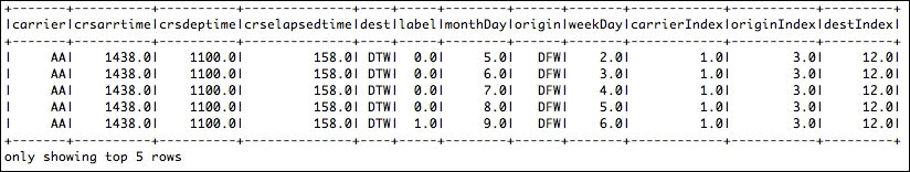
Figure 4: Uunique indices for each unique text

Step 2: Making the feature vectors using the vector assembler

Make the feature vector with the vector assembler and transform it to the labelled vector for applying the machine learning algorithm (decision tree). Note, here we used the decision tree to show just an example since it shows better classification accuracies. Based on the algorithm and model selection and tuning, you will be further able to explore and use other classifiers:

VectorAssembler assembler = new VectorAssembler().setInputCols( 
        new String[] { "monthDay", "weekDay", "crsdeptime", 
            "crsarrtime", "carrierIndex", "crselapsedtime", 
            "originIndex", "destIndex" }).setOutputCol( 
        "assembeledVector"); 

Now transform the assembler into a Dataset of row as follows:

Dataset<Row> assembledFeatures = assembler.transform(destIndexed); 

Now convert the Dataset into JavaRDD for making the feature vectors as follows:

JavaRDD<Row> rescaledRDD = assembledFeatures.select("label","assembeledVector").toJavaRDD(); 

Map the RDD for LabeledPoint as follows:

JavaRDD<LabeledPoint> mlData = rescaledRDD.map(new Function<Row, LabeledPoint>() { 
          @Override 
          public LabeledPoint call(Row row) throws Exception { 
            double label = row.getDouble(0); 
            Vector v = row.getAs(1); 
            return new LabeledPoint(label, v); 
          } 
        }); 

Now print the first five values as follows:

System.out.println(mlData.take(5));  

[Output]:

Figure 5: The corresponding assembled vectors

Here we will prepare the training dataset from the dataset of the labeled vector. Initially, we will make a training set where 15% of records will be non-delayed and 85% will be delayed records. Finally, the training and testing dataset will be prepared as 70% and 30% respectively.

Step 1: Make training and test set from the whole Dataset

First, create a new RDD by filtering the RDD based on the labels (that is, 1 and 0) we created previously as follows:

JavaRDD<LabeledPoint> splitedData0 = mlData.filter(new Function<LabeledPoint, Boolean>() { 
          @Override 
          public Boolean call(LabeledPoint r) throws Exception { 
              return r.label() == 0; 
          } 
        }).randomSplit(new double[] { 0.85, 0.15 })[1]; 
 
    JavaRDD<LabeledPoint> splitedData1 = mlData.filter(new Function<LabeledPoint, Boolean>() { 
          @Override 
          public Boolean call(LabeledPoint r) throws Exception { 
            return r.label() == 1; 
          } 
        }); 
   
    JavaRDD<LabeledPoint> splitedData2 = splitedData1.union(splitedData0); 
    System.out.println(splitedData2.take(1)); 

Now union the two RDDs using the union() method as follows:

JavaRDD<LabeledPoint> splitedData2 = splitedData1.union(splitedData0); 
System.out.println(splitedData2.take(1)); 

Now further convert the combined RDD into Dataset of Row as follows (max categories is set to be 4):

Dataset<Row> data = spark.sqlContext().createDataFrame(splitedData2, LabeledPoint.class); 
data.show(100); 

Now we need to do the vector indexer for the categorical variables as follows:

VectorIndexerModel featureIndexer = new VectorIndexer() 
          .setInputCol("features") 
          .setOutputCol("indexedFeatures") 
          .setMaxCategories(4) 
          .fit(data); 

Now that we have the feature indexer using the VectorIndexerModel estimator. Now the next task is to do the string indexing using the StringIndexerModel estimator as follows:

StringIndexerModel labelIndexer = new StringIndexer() 
          .setInputCol("label") 
          .setOutputCol("indexedLabel") 
          .fit(data); 

Finally, split the Dataset of Row into training and test (70% and 30% respectively but you should adjust the values based on your requirements) set as follows:

Dataset<Row>[] splits = data.randomSplit(new double[]{0.7, 0.3}); 
Dataset<Row> trainingData = splits[0]; 
Dataset<Row> testData = splits[1]; 

Well done! Now our dataset is ready to train the model, right? For the time being, we will naively select a classifier to say let's use the decision tree classifier to solve our purpose. You can try this with other multiclass classifiers based on examples provided in Chapter 6, Building Scalable Machine Learning Pipelines, Chapter 7, Tuning Machine Learning Models, and Chapter 8, Adapting Your Machine Learning Models.

As shown in Figure 2, training and test data will be collected from the raw data. After the feature engineering process has been done, the RDD of feature vectors with labels or ratings will be used next to be processed by the classification algorithm before building the predictive model (as shown in Figure 6) and at the end the test data will be used for testing the model performance:

Figure 6: Supervised learning using Spark

Next, we prepare the values for the parameters that will be required for the decision tree. You might have wondered why we are talking about the decision tree. The reason is simple since using the decision tree (that is, the binary decision tree)we observed better prediction accuracy compared to the Naive Bayes approaches. Refer to Table 2 which describes the categorical features and their significance as follows:

Table 2: Categorical features and their significance

Now we will describe the approach of the decision tree construction in brief. We will use the CategoricalFeaturesInfo that specifies which features are categorical and how many categorical values each of those features can take during the tree construction process. This is given as a map from the feature index to the number of categories for that feature.

However, the model is trained by making associations between the input features and the labeled output associated with those features. We train the model using the DecisionTreeClassifier method which returns a DecisionTreeModel eventually as shown in Figure 7. The detailed source code for constructing the tree will be shown later in this section:

Figure 7: The binary decision tree generated for the air-flight delay analysis (partially shown)

Step 1: Train the decision tree model

To train the decision tree classifier model, we need to have the necessary labels and features:

DecisionTreeClassifier dt = new DecisionTreeClassifier() 
      .setLabelCol("indexedLabel") 
      .setFeaturesCol("indexedFeatures"); 

Step 2: Convert the indexed labels back to original labels

To create a decision tree pipeline, we need to have the original labels apart from the indexed labels. So, let's do it as follows:

IndexToString labelConverter = new IndexToString() 
      .setInputCol("prediction") 
      .setOutputCol("predictedLabel")         
        .setLabels(labelIndexer.labels());  

Step 3: Chain the indexer and tree in a single pipeline

Create a new pipeline where the stages are as follows: labelIndexer, featureIndexer, dt, labelConverter as follows:

Pipeline pipeline = new Pipeline() 
      .setStages(new PipelineStage[]{labelIndexer,  
        featureIndexer, dt, labelConverter}); 

Now fit the pipeline using the training set we created in Step 8 as follows:

PipelineModel model = pipeline.fit(trainingData); 

Here we will test the models as shown in the following steps:

Step 1: Make the prediction on the test dataset

Make the prediction on the test set by transforming the PipelineModel and show the performance parameters as follows:

Dataset<Row> predictions = model.transform(testData); 
predictions.select("predictedLabel", "label", "features").show(5); 

Step 2: Evaluate the model

Evaluate the model by the multiclass classification evaluator and print the accuracy and test error as follows:

MulticlassClassificationEvaluator evaluator = new MulticlassClassificationEvaluator() 
      .setLabelCol("indexedLabel") 
      .setPredictionCol("prediction") 
      .setMetricName("accuracy"); 
    double accuracy = evaluator.evaluate(predictions); 
    System.out.println("accuracy: "+accuracy); 
    System.out.println("Test Error = " + (1.0 - accuracy)); 

The preceding code segment produces the classification accuracy and test error as follows:

Accuracy: 0.7540472721385786 
Test Error = 0.24595272786142142 

Please note that since we randomly split the dataset into training and testing, you might get a different result. The classification accuracy is 75.40%, which is not good, we believe.

However, now it's your turn to use a different classifier and tune before deploying the model. A more details discussion will be carried out in Chapter 7, Tuning Machine Learning Models, regarding tuning the ML models.

Step 3: Print the decision tree

Here is the code to print the decision tree:

DecisionTreeClassificationModel treeModel = 
      (DecisionTreeClassificationModel) (model.stages()[2]); 
System.out.println("Learned classification tree model:
" + treeModel.toDebugString()); 

This code segment produces a decision tree as shown in Figure 7.

Step 4: Stop the Spark session

Stop the Spark session using the stop() method of Spark as follows:

spark.stop();

This is a good practice that you initiate a Spark session and close or stop it properly to avoid the memory leak in your applications.