Answers to Selected Exercises
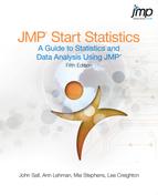
1a. (left) and 1b. (right)
1c. (left) - the Period2 linearized the data, and 1d. (right), the line of best fit
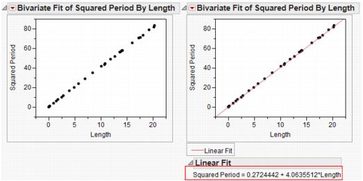
1e.  , so
, so 
1f. Enter the formula below (left) into a new column, then make another new column to find the difference between observed and theoretical period values (right).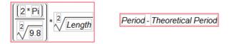
Use the Distribution platform to get the following histogram:

1g. This histogram reveals that the students measurements are higher than the theoretically predicted values.
2b. For each column, select the statistic from the Statistical Functions group in the Formula Editor.
2c. The multivariate plot shows some correlation among the mean, minimum, and maximum, and among the standard deviation, minimum, and maximum.

2e. Minimum and Maximum yield the following using Scatterplot 3D.
3a. The value converges to  , the golden ratio.
3c. It converges to the same number.
3d. Again, it converges to the same number.
3e. This time, the numbers converge to ¼.
1a. Levels and counts are shown in the Frequencies section of the report.

1b. The grosses range from $100 million to $600.8 million with an average gross of $157.5 million.

1d. To create the subset, use one of the following methods:
• To create the subset, use Rows > Row Selection > Select Where and complete the dialog to select where Type equals Drama. Then, use Tables > Subset to create the data table.
• Return to the Distribution of Type, and double-click on the bar for Drama.

2a. The following picture has the males highlighted. There are far more females for drug A than males.

2b. To produce this report, select Analyze > Distribution, assign pain to Y, Columns and drug to By. Select Uniform Scaling from the top red triangle menu for each distribution. The means do not appear to be the same.

3a. High calculus scores do seem to correlate with high physics scores.

3b. To produce the relevant report, select Calculus Score as Y, Columns and Region as By. The means for the four regions are 467.54, 445.1, 464.9, and 441.27 respectively.
3c. The mean Physics scores for each of the four regions are 424.1, 404.8, 427.9, and 417.4 respectively.
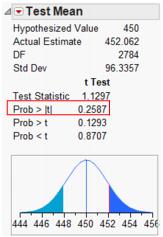
3d. After requesting a distribution of the scores, use the Test Mean command from the platform menu to test that the mean is not 450. The following report appears, showing that there is not evidence that the mean is different from 450.
3e. The confidence interval is shown in the Summary Statistics section of the calculus score report in question 3a as Lower 95% Mean and Upper 95% Mean (448.48, 455.64).
3f. After requesting a distribution of the scores, use the Test Mean command from the platform menu. The resulting report shows that the mean appears to be less than 420.

3g. The confidence interval is shown in the Moments section of the physics score report in question 3a (414.9, 419.33).
4a. The mean is 1.44 g. Three cereals, “100% Natural Bran Oats & Honey”, “Banana Nut Crunch”, and “Cracklin’ Oat Bran” appear to have unusually high amounts of fat.
4b. “All Bran with Extra Fiber” and “Fiber One”
4c. Cold cereals: (8.15g, 10.78g); Hot cereals (-2.46g, 5.13g). Note that there are only three hot cereals in the data set.
5a. Auto and Robbery seem to be skewed. The others have a more of a bell-shaped appearance.
5b. Nevada and New York
8a. A matched pairs approach is more appropriate, since these are repeated measures over time.
8b. The Matched Pairs platform yields the following report, showing a significant difference between the two months at a significance level of 0.05 (on the left, below).

c. There is no evidence for a significant difference between August and June (middle, above). Similarly, there is no evidence for a difference between August and March (right, above).
2b. There does not appear to be strong evidence between the two (p-value is 0.1218). However, sample size is small. The result is marginal and deserves further investigation.

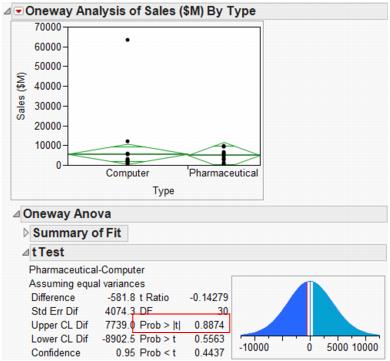
3a. The histograms are shown here. Note the outlier in the sales column and the skewed nature of the distribution.

3b. Grouped means are appropriate in this situation.
3c. Using Fit Y by X with Sales as Y and Type as X allows for the pooled or unpooled two-sample t-Test. The Means/Anova/ Pooled t command, which produces the report shown below, does not show evidence of a difference. Similarly, using the unpooled t Test command also does not show evidence of a difference.
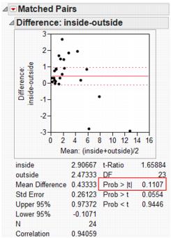
5b. The following report comes from the Matched Pairs platform. The p-value of 0.11 is a nonsignificant value.
1a. There are five levels. There are not an equal number of movies of each type (more Drama, fewer Mystery-Suspense).

1b. The null hypothesis is that the average Worldwide $ for different types of movies is the same. With a p-value of 0.0020 there is evidence for a difference between at least two movie types.
1c. Action and Drama are not different from all other movie types - they are both significantly different from Comedy.
1d. Since the lines in the Normal Quantile Plot appear to have very different slopes, a Welch anova is not a bad idea.

The output form the UnEqual Variances command shows four tests that the variances are unequal. Three support the conclusion that they are not equal. The Welch anova shows a similar conclusion to the parametric anova: there is a difference among the movie types.
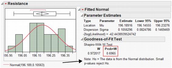
2a. After examining the histograms, Fit Distribution > Normal overlays a normal curve. Select Goodness of Fit from the Fitted Normal red triangle menu. The null hypothesis is stated in the Goodness-of-Fit Test results. The data appear to be normal.
2b. The null hypothesis is that there is no difference in the mean resistance for the different instruments. Fit Y by X is used to generate the anova shown here. There is no evidence that the instruments differ.

3a. 299,852.4 km/sec
3b. There is evidence that the trials differ.

3c. The first set of observations is higher than the others on average.

3d. Excluding the first group and re-computing the mean results in a mean of 299838.25, which is closer to the true value of 299792.5 km/sec.
4b. All three give the same (significant) result.

4c. An anova shows a non-significant result.
5a. There is a difference among the regions for Calculus scores.
5b. There is a difference among the regions for Physics scores.
5c. Groups 1 and 3 appear to be quite different from groups 2 and 4.
1a. One movie (Titanic) is definitely separated from the rest of the movies.

1b and 1c. The linear model does explain the data better than the simple mean model. (Why?)

1d. The model with excluded outliers is probably a better summary of a typical movie’s performance.
1e (left) and 1f (right). There are differences in gross dollars for the different types of movies.

1g. The regression lines for the two types of movies are different.

2a. The mean for 1996 is about 10 points higher than for the other two elections.

Perhaps 1996 (Clinton vs. Dole) was a more contested election than the others (Reagan vs. Carter, Reagan vs. Mondale).
2b. 1984 vs. 1980: 0.704. 1996 vs 1980: 0.593. Correlations are stronger for years that are closer together.

2c. Probably not. The next presidential election is far removed from 1996, 1984, and 1980.
3a. Afghanistan, Angola and Mozambique are outliers for the death rate variable.
3b.The line is a better predictor than the mean, but a line is not an appropriate model (see part d of this question).
3c. There is a u-shaped pattern to these residuals (in the first two, shown on the left below).

d. Because of the pattern of the residuals (and, actually, the pattern of the original data—clearly nonlinear), a line is not an appropriate model.
4a. 1-Octanol
4b. Right-click on the Parameter Estimates report and select Columns > Lower 95% and Columns Upper 95% to reveal the confidence interval we want.

1a. The Test Probabilities command from the Distribution report gives the following results:

Based on these numbers, there’s no reason to dispute the company’s claim.
2. We entered the data into two columns of a data table, one representing the machines and the second representing the counts. Then, we selected Analyze > Distribution with Machine as Y and the counts as Freq. In the Distribution report we used Test Probabilities to test that they were all the same.

They clearly are different.
1a. Use Analyze > Fit y by X, with Gender as X and Grades as Y. There is no significant difference.

1b. Yes

1c. Looks: Yes; Money: No
1d. Grades: No; Sports: No; Looks: No; Money: No
2. Create a data table, as shown below. Then, use Analyze > Fit Y by X with Absorbency as Y, Acid as X and Count as Freq.

There is evidence of a difference in absorbency between the two acids.
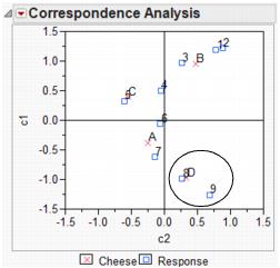
3a and 3b: The Mosaic Plot and the tests indicate that there is a difference in additives.
3c. Cheese D is associated with high tasted scores. Cheese A comes in second.
 .
.4a, 4b, and 4c. See the counts below.
4d (left) and 4e (right). Both passenger class and sex are significant. There are differences in the survival rate for different passenger classes and different sexes.
4f. Age is marginally significant, with a p-value of 0.0720.

Note: For a better model, use Fit Model with multiple Xs.
1a. 0.533
1b. Yes, it increases to 0.893.
2b. The effect with the least significance is Shoulder, which has a p-value of 0.90.
2c. After several repetitions, Fore, Waist, Height, and Thigh remain in the model.
2d. We reach an identical model.
3a. Dreaming and Non-Dreaming. Note that this model is degenerate since there is no variability in Dreaming that is not accounted for by the Non-Dreaming variable.
3b. Dreaming and Exposure.
3c. The R2 is 0.934.
3d. Forward stepwise gives a model with Dreaming, Gestation, and Danger.
3e. Mixed stepwise gives the same model as part d.
1a. The Summary of Fit and Analysis of Variance tables are the same in both platforms (below, Fit Y by X is shown left, and Fir Model is right).

1b. This plot (like the comparison circles) tell us that Caustic Soda and Pumice Stone remove more starch than Alpha Amalyze.

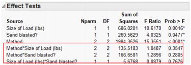
1c. All effects are significant.
1d. The Method LS means for Method is identical to the one in part (b). The Sand Blasted plot indicates that sand blasting removes more starch than not.
1e. It is (F = 28.66, p < 0.001).
1f. No interaction effects are significant.
2b. The model predicted correctly about 78% of the time - (520 + 301)/1046.
2c. All of the two-way interactions are significant.
1b. Only main effects and two-way interactions are significant.
1d. The optimal settings are below. Results are the same as the 20 run reactor experiment.
2a. 5 levels for each factor.
2b. Optimal settings are below. The goals were met for HARDNESS and ELONG. The model didn’t do as well in maximizing ABRASION.
1a. Most of the variables are positively correlated. Alaska, Mass and New York are outliers.
1c. Auto theft and robbery are close together. Murder is by itself.
1d. 2 or 3

3. JMP produces a model that misclassifies only three flowers.

4. The distance plot suggests around 4 clusters.
2a. Minimization of Time appears at Length=2.5, Freq=250, and Space = 0.721. This is from using the following model.

1a. An XBar R or S is appropriate. There were multiple readings per hour.
1b and 1c. The mean is 8.1053. The process appears stable. No special causes signal.

2a. In question 1 we saw that the process is stable, and the underlying distribution is normal.
2b and 2c. 3.33% fell outside the spec limits. 5.4% are predicted in the long term.
2d. The process is not capable. The CPK is below 1.0.
2e. The process is on target. Engineers should focus on variability reduction.

..................Content has been hidden....................
You can't read the all page of ebook, please click here login for view all page.