
Chapter 6
Finite Elements for Two‐Dimensional Solid Mechanics
6.1 INTRODUCTION
All real‐life structures are three–dimensional. It is engineers who make the approximation as a one‐dimensional (e.g., beam) or a two‐dimensional structure (e.g., plate or plane solid). In chapter 5 we explained in detail the conditions under which such approximation could be made. When the stresses on a plane normal to one of the axes are approximately zero, then we say that the solid is in the state of plane stress. Similarly, when the corresponding strains are zero, the solid is in the state of plane strain. A two‐dimensional solid is also called a plane solid. Some examples of plane solids are: (1) a thin plate subjected to in‐plane forces; or (2) a very thick solid with a constant cross‐section in the thickness direction. In this chapter, we will discuss when an engineering problem can be assumed to be two‐dimensional and how to solve such a problem using two‐dimensional finite elements. We will introduce three different types of two‐dimensional problems and corresponding two‐dimensional elements. Every element has its own characteristics. In order to use the finite element method appropriately, a thorough understanding of the capabilities and limitations of each element is required.
In general, two‐dimensional elasticity problem can be expressed by a system of coupled second‐order partial differential equations. Based on the constraints imposed in the thickness direction, a two‐dimensional problem can be a plane stress or plane strain problem. The main difference is in the stress‐strain relations. Yet another type of problem that can be classified as two‐dimensional is the axisymmetric problem where the structure has symmetry about an axis and it deforms only in the radial and axial directions.
In an elasticity problem, the main variables are the displacements in the coordinate directions. After solving for the displacements, stresses and strains can be calculated from the derivatives of displacements. The displacements are calculated using the fact that the structure is in equilibrium when the total potential energy has its minimum value. This will yield a matrix equation similar to the beam problem in chapter 3.
6.2 TYPES OF TWO‐DIMENSIONAL PROBLEMS
6.2.1 Governing Differential Equations
In two‐dimensional problems, the stresses and strains are independent of the coordinate in the thickness direction, (usually the z‐axis). By setting all the derivatives with respect to the z‐coordinate in eq. (5.69) in chapter 5 to zero, we obtain the governing differential equations for plane problems as

where bx and by are the body forces.
Let u and v be the displacement in the x‐ and y‐direction, respectively. From eqs. (5.39)–(5.45), the strain components in a plane solid are defined as

In addition, the stresses and strains are related by the following constitutive relation:

Substituting the stress‐strain relations in eq. (6.3) and strain‐displacement relations in eq. (6.2) in the equilibrium equations in eq. (6.1), we obtain a pair of second‐order partial differential equations in two variables u(x,y) and v(x,y). The explicit form of the equations is available in textbooks on elasticity, for instance, Timoshenko and Goodier1.
The differential equation must be accompanied by boundary conditions. Two types of boundary conditions can be defined. The first one is the boundary in which the values of displacements are prescribed (essential boundary condition). The other is the boundary in which the tractions are prescribed (natural boundary condition). The boundary conditions can be formally stated as

where Sg and ST, respectively, are the boundaries where the displacement and traction boundary conditions are prescribed. The objective is to determine the displacement field u(x,y) and v(x,y) that satisfies the differential equation (6.1) and the boundary conditions in eq. (6.4). Now, we will discuss the stress‐strain relations in eq. (6.3) for the two different plane problems—plane stress and plane strain. The third type of 2D problem, namely axisymmetric problems, will be discussed later in the chapter.
6.2.2 Plane Stress Problems
Plane stress conditions exist when the thickness dimension (usually the z‐direction) is much smaller than the length and width dimensions of a solid. Since stresses at the two surfaces normal to the z‐axis are zero, it is assumed that stresses in the normal direction are zero throughout the body, that is, σzz = τxz = τyz = 0. In such a case, the structure can be modeled in two dimensions. An example of the plane stress problem is a thin plate or disk with applied in‐plane forces (see figure 6.1).
- – Nonzero stress components: σxx, σyy, τxy.
- – Nonzero strain components: εxx, εyy, γxy, εzz.

Figure 6.1 Thin plate with in‐plane applied forces
Under plane stress conditions, for linear isotropic materials, the stress‐strain relation can be written as (see section 5.3)

where [Cσ] is the stress‐strain matrix or elasticity matrix for the plane stress problem. It should be noted that the normal strain εzz in the thickness direction is not zero; it can be calculated from the following relation:
6.2.3 Plane Strain Problems
A state of plane strain will exist in a solid when the thickness dimension is much larger than other two dimensions. When the deformation in the thickness direction is constrained, the solid is assumed to be in a state of plane strain even if the thickness dimension is small. A proper assumption is that strain components with z subscript are zero, that is, εzz = γxz = γyz = 0. In such a case, it is sufficient to model a slice of the solid with unit thickness. Some examples of plane strain problems are the retaining wall of a dam and long cylinder such as a gun barrel (see figure 6.2).
- – Nonzero stress components: σxx, σyy, τxy, σzz.
- – Nonzero strain components: εxx, εyy, γxy.

Figure 6.2 Dam structure with plane strain assumption
For linear isotropic materials, the stress‐strain relations under plane strain conditions can be written as (see section 5.3)

where [Cε] is the stress‐strain matrix for the plane strain problem. It should be noted that the transverse stress σzz is not equal to zero in the plane strain case, and it can be calculated from the following relation:
6.2.4 Equivalence between Plane Stress and Plane Strain Problems
Although plane stress and plane strain problems are different by definition, they are quite similar from the computational viewpoint. Thus, it is possible to use the plane strain formulation and solve the plane stress problem. In such case, two material properties, E and ν, need to be modified. Similarly, it is also possible to convert the plane stress formulation into the plane strain formulation. Table 6.1 summarizes the conversion relations.
Table 6.1 Material property conversion between plane strain and plane stress problems
| From → To | E | ν |
| Plane strain → Plane stress |  |
|
| Plane stress → Plane strain |  |
6.3 CONSTANT STRAIN TRIANGULAR (CST) ELEMENT
In finite element analysis, a plane solid can be divided into a number of contiguous elements. In chapter 4, we introduced the 3‐node triangular element for heat transfer problems. In this section, we will use the same element for plane solid problems. Figure 6.3 shows a typical mesh consisting of triangular elements. The three nodes of the element, as shown in figure 6.3, have two displacement components, u and v, respectively in the x‐ and y‐direction for two‐dimensional solid mechanics problems. The first node of an element can arbitrarily be chosen. However, the sequence of the nodes 1, 2, and 3 should be in the counterclockwise direction.

Figure 6.3 Constant strain triangular (CST) element
The nodal values of the displacement components are interpolated within the element using shape functions. In the polynomial approximation, the displacement has to be a linear function in x and y because displacement information is available only at three points (nodes), and a linear polynomial has three unknown coefficients. Since displacement is a linear function, strain and stress are constant within an element, and that is why a triangular element is called a constant strain triangular element.
6.3.1 Displacement and Strain Interpolation
The first step in deriving the finite element matrix equation is to interpolate the displacement function within the element using the nodal values of displacements. Let the x‐ and y‐directional displacements be u(x,y) and v(x,y), respectively. Since the two coordinates are perpendicular to each other (orthogonal), u(x,y) and v(x,y) are independent of each other. Hence, u(x,y) needs to be interpolated in terms of u1, u2, and u3, and v(x,y) in terms of v1, v2, and v3. It is obvious that the interpolation function must be a three‐term polynomial in x and y. Since we must have rigid body displacements (constant displacements) and constant strain terms in the interpolation function, the displacement interpolation must be of the following form:

where α’s and β’s are constants. In finite element analysis, we would like to replace the constants by the nodal displacements. Let us consider x‐directional displacements, which are u1, u2, and u3. At node 1, for example, x and y take the values of x1 and y1, respectively, and the nodal displacement is u1. If we repeat this for other two nodes, we obtain the following three simultaneous equations:

In matrix notation, the above equations can be written as

If the three points (x1, y1), (x2, y2), and (x3, y3) are not on a straight line, then the inverse of the above coefficient matrix exists. Thus, we can calculate the unknown coefficients as

where A is the area of the triangle and

The area A of the triangle can be calculated from

Note that the determinant in eq. (6.14) is zero when three nodes are collinear. In such a case, the area of the triangular element is zero, and we cannot uniquely determine the three coefficients.
A similar procedure can be applied to the y‐directional displacement v(x, y), and the unknown coefficients βi, (i = 1, 2, 3) are determined using the following equation:

After calculating αi and βi, the displacement interpolation can be written as

where the shape functions are defined by

Note that N1, N2, and N3 are linear functions of x‐ and y‐coordinates. Thus, interpolated displacement varies linearly in each coordinate direction.
In order to make the derivations simple, we will rewrite the interpolation relation in eq. (6.16) in matrix form. Let {u} = {u, v}T be the displacement vector at any point (x, y). The interpolation can be written in the matrix notation by
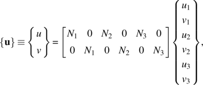
or
Equation (6.18) is the critical relationship in finite element approximation. When a point (x, y) within a triangular element is given, the shape function [N] is calculated at this point. Then, the displacement at this point can be calculated by multiplying this shape function matrix with the nodal displacement vector {q}. Thus, if we solve for the nodal displacements, we can calculate the displacement everywhere in the element. Note that the nodal displacements will be evaluated using the principle of minimum total potential energy in the following section.
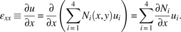
After calculating displacement within an element, it is possible to calculate the strain by differentiating the displacement with respect to x and y. From the expression in eq. (6.18), it can be noted that the nodal displacements are constant, but the shape functions are functions of x and y. Thus, the strain can be calculated by differentiating the shape function with respect to the coordinates. For example, εxx can be written as
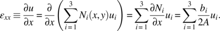
Note that u1, u2, and u3 are nodal displacements, and they are independent of coordinate x. Thus, only the shape function is differentiated with respect to x. A similar calculation can be carried out for εyy and γxy. Using the matrix notation, we have

It may be noted that the [B] matrix is constant and depends only on the coordinates of the three nodes of the triangular element. Thus, one can anticipate that if this element is used, then the computed strains will be constant over a given element and will depend only on nodal displacements. Hence, this element is called the Constant Strain Triangular Element or CST element. The interpolation of displacement in eq. (6.18) and the expression for strain in eq. (6.20) are used for approximating the strain energy and potential energy of applied loads.
6.3.2 Properties of the CST Element
Before we derive the strain energy, it may be useful to study some interesting aspects of the CST element. Since the displacement field is assumed to be a linear function in x and y, one can show that the triangular element deforms into another triangle when forces are applied. Furthermore, an imaginary straight line drawn within an element before deformation becomes another straight line after deformation.
Let us consider the displacements of points along one of the edges of the triangle. Consider the points along the edge 1–2 in figure 6.4. These points can be conveniently represented by a coordinate ξ. The coordinate ξ = 0 at node 1 and ξ = a at node 2. Along this edge, x and y are related to ξ. By substituting this relation in the displacement functions, one can express the displacements of points on the edge 1–2 as a function of ξ. It can be easily shown that the displacement functions, for both u and v, must be linear in ξ, that is,

where γ’s are constants to be determined. Since the variation of displacement is linear, it might be argued that the displacements should depend only on u1 and u2, and not on u3. Then, the displacement field along the edge 1‐2 takes the form:

where H1 and H2 are shape functions defined along the edge 1‐2, and a is the length of edge 1‐2. One can also note that a condition called inter‐element displacement compatibility is satisfied by triangular elements. This condition can be described as follows: any point should have a unique displacement including along shared edges between elements. After the loads are applied and the solid is deformed, the displacements at any point in an element can be computed from the nodal displacements of that particular element and the interpolation functions in eq. (6.18). Consider a point on a common edge of two adjacent elements. This point can be considered as belonging to either of the elements. Then the nodes of either triangle can be used in interpolating the displacements of this point. However, one must obtain a unique set of displacements independent of the choice of the element. This can be true only if the displacements of the points depend only on the nodes common to both elements. In fact, this will be satisfied because of eq. (6.21). Thus, the CST element satisfies the inter‐element displacement compatibility.

Figure 6.4 Inter‐element displacement compatibility of constant strain triangular element
Note that the displacements are linear and the strains are constant in each element. From the given nodal displacements, it is clear that the top edge has strain εxx = −0.2, while the bottom edge has εxx = 0.2. The strain varies linearly along the y‐coordinate. However, the triangular element cannot represent this change, and provides constant values of εxx = 0.2 for element 1 and εxx = −0.2 for element 2. In general, if a plane solid is under the constant strain states, the CST element will provide accurate solutions. However, if the strain varies in the solid, then the CST element cannot represent it accurately. In such a case, a dense mesh with many elements should be used to approximate it as a series of step functions. Note that the strains along the interface between two elements are discontinuous.
6.3.3 Strain Energy
Let us calculate the strain energy in a typical triangular element, say element e. In eq. (5.72), the strain energy of the plane solid was derived in terms of strains and the elasticity matrix [C]. Substituting for strains from eq. (6.20), we obtain

where [k(e)] is the element stiffness matrix of the triangular element. The column vector {q(e)} contains the displacements of the three nodes that belong to the element. The dimension of [k(e)] is 6 × 6. In the case of the triangular element, all entries in matrices [B] and [C] are constant and can be integrated easily. After integration, the element stiffness matrix takes the form

where A(e) is the area of the plane element. Using the expression for [B] in eq. (6.20) and stress–strain relation in eq. (6.5), the element stiffness matrix can be calculated.
One may note that in the case of truss and frame elements, we used a transformation matrix [T] in deriving the element stiffness matrix. However, in the present case, we have used the global coordinate system in the derivation of [k(e)], and that is the reason for not using a transformation matrix. In some cases, however, it is required to define the element in a local coordinate system. For example, if the material is not isotropic, it will have a specific directional property. In such a case, [k(e)] is first derived in a local coordinate system and transformed to the global coordinates by multiplying by appropriate transformation matrices.
The strain energy of the entire solid is simply the sum of the element strain energies. That is,

where NEL is the number of elements in the model. The superscript (e) in q(e) implies that it is the vector of displacements or DOFs of element e. The summation in the above equation leads to the assembling of the element stiffness matrices into the global stiffness matrix.
where {Qs} is the column vector of all displacements in the model and [Ks] is the structural stiffness matrix obtained by assembling the element stiffness matrices.
6.3.4 Potential Energy of Applied Loads
Concentrated forces at nodes:
The next step is to calculate the potential energy of external forces. We will consider three different types of applied forces. The first type is concentrated forces at nodes. It may be noted that the model expects two forces, one in the x‐direction and the other in the y‐direction, at each node. In general, the potential energy of concentrated nodal forces can be written as
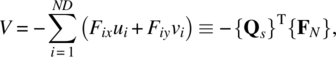
where ![]() is the vector of applied nodal forces, and ND is the number of nodes in the solid. The contribution of a particular node to the potential energy will be zero if no force is applied at the node, or the displacement of the node becomes zero. The above potential energy of concentrated forces does not include a supporting reaction because the displacement at those nodes will be zero.
is the vector of applied nodal forces, and ND is the number of nodes in the solid. The contribution of a particular node to the potential energy will be zero if no force is applied at the node, or the displacement of the node becomes zero. The above potential energy of concentrated forces does not include a supporting reaction because the displacement at those nodes will be zero.
Distributed forces along element edges:
The second type of applied force is the distributed force (traction) on the side surface of the plane solid. In the plane solid, the traction is assumed to be a constant through the thickness. Let the surface traction force {T} = {Tx, Ty}T is applied on the element edge 1‐2 as shown in figure 6.6. The unit of the surface traction is Pa (N/m2) or psi. Since the force is distributed along the edge, the potential energy of the surface traction force must be defined in the form of integral as

where ![]() is the vector of displacements along the edge 1‐2,
is the vector of displacements along the edge 1‐2, ![]() is the vector of applied tractions along the edge 1‐2,
is the vector of applied tractions along the edge 1‐2, ![]() is the vector of displacements of nodes 1 and 2, and
is the vector of displacements of nodes 1 and 2, and

is the matrix of shape functions defined in eq. (6.21). The integration can be performed in a closed form if the specified surface tractions (Tx and Ty) are simple functions of s. We will modify eq. (6.27) to include all the six DOFs of the element and rewrite as

We have used the complete shape function matrix in eq. (6.28):


Figure 6.6 Applied surface traction along edge 1‐2
If the last expression in eq. (6.28) is examined carefully, it is possible to note that the force vector {fT} is nodal force vector that is equivalent to the distributed force applied on the edge of the element. This is also called the work‐equivalent nodal force vector. For a constant surface traction Tx and Ty, we can calculate the equivalent nodal force, as

For the uniform surface traction force, the equivalent nodal forces are obtained by simply dividing the total force equally between the two nodes on the edge.
The potential energy of distributed forces of all elements whose edge belongs to the traction boundary ST must be assembled to build the global force vector of distributed forces:
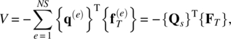
where NS is the number of elements whose edge belongs to ST.
Body forces:
The body forces are distributed over the entire element (e.g., centrifugal forces, gravitational forces, inertia forces, or magnetic forces). For simplification of the derivation, let us assume that a constant body force b = {bx, by}T is applied to the whole element. The potential energy of body force becomes

where

The resultant of body forces is hAbx in the x‐direction and hAby in the y‐direction. Equation (6.33) equally distributes these forces to the three nodes. Similar to the distributed force, {fB} is the equivalent nodal force corresponding to the constant body force.
The potential energy of body forces of all elements must be assembled to build the global force vector of body forces:

where NEL is the number of elements.
6.3.5 Global Finite Element Equations
Since the strain energy and potential energy of applied forces are now available, let us go back to the potential energy of the triangular element. The discrete version of the potential energy becomes
The principle of minimum potential energy in chapter 2 states that the structure is in equilibrium when the potential energy is minimum. Since the potential energy in eq. (6.35) is a quadratic form, the displacement vector {Qs}, we can differentiate Π to obtain

The stationary condition of the potential energy yields the global finite element matrix equations.
The assembled structural stiffness matrix [Ks] is singular due to the rigid body motion. After constructing the global matrix equation, the boundary conditions are applied by removing those DOFs that are fixed or prescribed. After imposing the boundary condition, the global stiffness matrix becomes nonsingular and it can be inverted to solve for the nodal displacements.
6.3.6 Calculation of Strains and Stresses
Once the nodal displacements are calculated, strains and stresses in individual elements can be calculated. First, the nodal displacement vector {q(e)} for the element of interest needs to be extracted from the global displacement vector. Then, the strains and stresses in the element can be obtained from
and
where [C] = [Cσ] for the plane stress problems and [C] = [Cε] for the plane strain problems.
As discussed before, stress and strain are constant within an element because matrices [B] and [C] are constant. This property can cause difficulties in interpreting the results of the finite element analysis. When two adjacent elements have different stress values, it is difficult to determine the stress value at the interface. Such discontinuity is not caused by the physics of the problem but by the inability of the triangular element in describing the continuous change of stresses across element boundary. In fact, most finite elements cannot maintain continuity of stresses across the element boundary. Most programs average the stress at the element boundaries in order to make the stress look continuous. However, as we refine the model using smaller‐size elements, this discontinuity can be reduced. The following example illustrates discontinuity of stress and strain between two adjacent CST elements.
From example 6.2, we can conclude the following:
- – Stresses are constant over the individual element.
- – The solution is not accurate because there are large discontinuities in stresses across element boundaries.
- – With only two elements, the mesh is very coarse, and we obviously cannot expect very good results.
6.4 FOUR–NODE RECTANGULAR ELEMENT
6.4.1 Lagrange Interpolation for a Rectangular Element
A rectangular element is composed of four nodes and eight DOFs (see figure 6.8). It is a part of a plane solid that is composed of many rectangular elements. Each element shares its edge and two corner nodes with an adjacent element, except for those on the boundary. The four vertices of a rectangle are the nodes of that element as shown in figure 6.8. The first node of an element can arbitrarily be chosen. However, the sequence of the nodes 1, 2, 3, and 4 should be in the counterclockwise direction. Each node has two displacements, u and v, respectively in the x‐ and y‐direction.

Figure 6.8 Four–node rectangular element
Since all edges are parallel to the coordinate directions, this element is not practical, but it is useful, as it is the basis for the quadrilateral element discussed in the following chapter. In addition, the behavior of the rectangular element is similar to that of the quadrilateral element. Shape functions can be calculated using procedures similar to that of CST element, but it is more instructive to use the Lagrange interpolation functions in the x‐ and y‐direction.
Consider the rectangular element in figure 6.8. From the geometry, it is clear that x3 = x2, y4 = y3, x4 = x1, and y2 = y1. We will use a polynomial in x and y as the interpolation function. Since there are four nodes, we can apply four boundary conditions, and hence the polynomial should have four terms as follows:

Let us calculate unknown coefficients αi using the x‐directional displacement u:

It is obvious that we need to invert the 4 × 4 matrix in order to calculate the interpolation coefficients.
Instead of matrix inversion method, we use the Lagrange interpolation method to interpolate u and v. The goal is to obtain the following expression:

where N1, …, N4 are the interpolation functions. In order to do that, let us first consider displacement along edge 1‐2 in figure 6.8. Along edge 1‐2, y = y1 (constant); therefore, shape functions must be functions of x only as shown below:

Using the one‐dimensional Lagrange interpolation formula, the shape functions can be obtained as
This is the same procedure that was used in chapter 2. Next, since y = y3 = y4 along edge 4‐3 in figure 6.8, the displacement can be interpolated as

Again from the one‐dimensional Lagrange interpolation formula, we have
Equations (6.41) and (6.43) represent interpolation of displacements at the top and bottom of the element, respectively. So far, we have interpolated displacements in the x‐direction only. Now, we can extend the interpolation in the y‐direction between uI(x,y1) and uII(x,y3) using the same Lagrange interpolation method. By considering uI(x,y1) and uII(x,y3) as nodal displacements, we have the following interpolation formula:

where
are the Lagrange interpolations in the y‐direction. By substituting eqs. (6.41) and (6.43) into eq. (6.45), we have the following formula:

Thus,

Comparing the above expression with eq. (6.40) we can define shape functions. N1, …, N4. In the rectangular element, it is enough to use the coordinates of two nodes, because x1 = x4, y1 = y2, and so forth. We will use the coordinates of nodes 1 and 3. Using the property that the area of the element is A = (x3 – x1)(y3 – y1), we obtain

Note that the shape functions for rectangular elements are the product of Lagrange interpolations in the two coordinate directions. Let us discuss the properties of the shape functions. It can be easily verified that N1(x, y) is:
- – 1 at node 1 and 0 at other nodes
- – a linear function of x along edge 1‐2 and linear function of y along edge 1‐4 (bilinear interpolation)
- – zero along edges 2‐3 and 3‐4
Other shape functions have similar behavior. Because of these characteristics, the i‐th shape function is considered associated with node i of the element.
In order to make the derivations simple, we rewrite the interpolation relation in eq. (6.40) in matrix form. Let {u} = {u, v}T be the displacement vector at any point (x, y). The interpolation can be written using the matrix notation by

or
Note that the dimension of the shape function matrix is 2 × 8.
Since the shape functions are given as a function of x‐ and y‐coordinates, we can use an approach similar to that of CST element to obtain the strain–displacement relations. Thus, the strain can be calculated by differentiating the shape function with respect to the coordinates. For example, εxx can be written as
Note that u1, u2, u3, and u4 are nodal displacements, and they are independent of coordinate x. Thus, only the shape function is differentiated with respect to x. Similar calculation can be carried out for εyy and γxy. Then, we have

Note that matrix [B] is a linear function of x and y. Thus, the strain will change linearly within the element. For example, εxx will vary linearly in the y‐direction, while it is constant with respect to x. Thus, the element will have approximation error, if the actual strains vary in the x‐direction.
6.4.2 Element Stiffness Matrix
The element stiffness matrix can be calculated from the strain energy of the element. By substituting for strains from eq. (6.52) into the expression for strain energy in eq. (6.52) we have

where [k(e)] is the element stiffness matrix. Calculation of the element stiffness matrix requires two‐dimensional integration. We will discuss numerical integration in the next chapter. When the element is square and the problem is plane stress, analytical integration of the strain energy yields the following form of element stiffness matrix:

It is interesting to note that the element stiffness matrix does not depend on the actual element dimensions, but it is a function only of material properties (E and ν) and thickness h.
The strain energy of the entire solid can be obtained using eq. (6.24), which involves the assembly process.
6.4.3 Potential Energy of Applied Loads
In the CST element, we discussed three different types of applied loads: concentrated forces at nodes, distributed forces along element edges, and body force. The first two types are independent of the element used. Thus, the same forms in eqs. (6.26) and (6.31) can be used for the potential energies of concentrated force and distributed force, respectively.
In the case of the body force, the element shape functions are used to calculate equivalent nodal forces. When a constant body force b = {bx, by}T acts on a rectangular element, the potential energy of body force becomes

where

Equation (6.56) equally divides the total magnitude of the body force to the four nodes. {fb} is the equivalent nodal force corresponding to the constant body force. The potential energy of body forces of all elements must be assembled to build the global force vector of body forces as in eq. (6.34).
Using the principle of minimum total potential energy in eq. (6.36), a similar global matrix equation for the rectangular elements can be obtained. Applying boundary conditions and solving the matrix equations are identical to those of the CST element. After solving for nodal displacements, strains and stresses in each element can be calculated using eqs. (6.37) and (6.38), respectively.
6.5 AXISYMMETRIC ELEMENT
Axisymmetric problems are also classified as two‐dimensional solid mechanics problems. For such problems, the structure has a geometry that is symmetric about an axis. For instance, cylinders and cones are axisymmetric geometries. Any structure where the geometry can be described as the volume swept by a two‐dimensional profile or section revolved about an axis is a structure with symmetry about that axis. If the applied loads and constraints on such geometry are also symmetric about the same axis, then the structure would deform in an axisymmetric manner. Even though all real structures are three‐dimensional, we can state the problem as two‐dimensional only if all the quantities of interest are constant in the direction normal to a plane and the displacement field has only two components that are parallel to this plane. In this case, the domain of the analysis is an area on this plane. For plane stress and plane strain problems, the thickness in the z‐direction is constant and we are able to easily convert volume integrals into area integrals because the field variables of interest are constant in the z‐direction.
Axisymmetric problems can also be stated as two‐dimensional problems when viewed with respect to a cylindrical coordinate system as shown in figure 6.15 where the geometry in (a) is obtained by revolving the section in (b). The section plane is on the r‐z plane and is the plane on which the displacement vector must lie. If the z‐axis is the axis of symmetry, then points on the r‐z plane must remain on this plane as the structure deforms in order for it to be considered a two‐dimensional deformation. Any twisting about the z‐axis will result in a three‐dimensional deformation.

Figure 6.15 Axisymmetric geometry; (a) revolved geometry, (b) section – plane of deformation
To summarize, the conditions under which we have axisymmetric deformation are:
- The geometry of the structure must be symmetric about an axis.
- The applied load and boundary conditions must also be symmetric about the same axis.
- The structure should not be subjected to loads that produce a torque about the axis of symmetry. In other words, the structure should not twist about the axis.
For an axisymmetric problem, the displacement field has two components (ur, uz) which are the radial and axial components in a cylindrical coordinate system. The component of displacement in the tangential or circumferential direction must be zero (![]() ). Any displacement in the circumferential direction would cause twisting about the axis, which is the reason for assuming that there is no torque applied about the axis. Even though there is no displacement in the θ ‐direction, there is a stress in this direction, often referred to as the hoop stress. To understand the reason for this stress, imagine a circle in the structure on a plane normal to the axis with its center at the axis of symmetry of the structure as shown in figure 6.16. During the deformation, if there is any displacement ur in the radial direction, this will cause the radius of the circle to increase, which implies that the circumference will increase resulting in a strain in the circumferential/tangential direction, which is the hoop strain, εθθ. This strain is an extensional strain and can be defined as the change in circumference over the original circumference of this circle as shown in the following equation.
). Any displacement in the circumferential direction would cause twisting about the axis, which is the reason for assuming that there is no torque applied about the axis. Even though there is no displacement in the θ ‐direction, there is a stress in this direction, often referred to as the hoop stress. To understand the reason for this stress, imagine a circle in the structure on a plane normal to the axis with its center at the axis of symmetry of the structure as shown in figure 6.16. During the deformation, if there is any displacement ur in the radial direction, this will cause the radius of the circle to increase, which implies that the circumference will increase resulting in a strain in the circumferential/tangential direction, which is the hoop strain, εθθ. This strain is an extensional strain and can be defined as the change in circumference over the original circumference of this circle as shown in the following equation.

Figure 6.16 Circumferential strain due to radial displacement
From the above discussion, it is clear that there are four strain components for axisymmetric problems. Similarly, there are four stress components: σrr the radial stress, σzz the axial stress, σθθ or the hoop stress, and finally τrz the shear stress. The strain components, placed in a column matrix, can be defined as:

For finite element analysis, within each element, we can compute the strains using the interpolated displacement components. For convenience we will use the notation: ![]() and
and ![]() . The nodal values of the displacement components can then be denoted as
. The nodal values of the displacement components can then be denoted as ![]() . We will assume that when modeling the two‐dimensional cross section, we will create the model on the xy‐plane such that the r‐ and z‐axis of the cylindrical coordinate system align with the x‐ and y‐axis of the Cartesian coordinates. Therefore, in the subsequent discussion, we will assume that
. We will assume that when modeling the two‐dimensional cross section, we will create the model on the xy‐plane such that the r‐ and z‐axis of the cylindrical coordinate system align with the x‐ and y‐axis of the Cartesian coordinates. Therefore, in the subsequent discussion, we will assume that ![]() and
and ![]() . The strain components can be numerically computed within each element as:
. The strain components can be numerically computed within each element as:

The preceding equation is valid for any two‐dimensional element with n nodes. The first two columns of the [B] matrix are multiplied by ![]() or the degrees of freedom of the first node, and the same pattern repeats for every node. The third row corresponds to the hoop strain, where the denominator is the distance of the point at which the strain is being computed from the axis of revolution. It appears as though the hoop strain could be undefined at the axis because the distance from the axis is zero along the axis. Indeed it would be infinite unless the numerator is also zero or in other words, points along the axis cannot have any displacement in the radial direction regardless of the applied loads. This makes sense when you consider that displacement of points at the axis in the radial direction is equivalent to a hole being created at the axis. Therefore, for axisymmetric problems, it is not necessary to add displacement boundary conditions in the radial direction on any edge of the domain that is along the axis of symmetry.
or the degrees of freedom of the first node, and the same pattern repeats for every node. The third row corresponds to the hoop strain, where the denominator is the distance of the point at which the strain is being computed from the axis of revolution. It appears as though the hoop strain could be undefined at the axis because the distance from the axis is zero along the axis. Indeed it would be infinite unless the numerator is also zero or in other words, points along the axis cannot have any displacement in the radial direction regardless of the applied loads. This makes sense when you consider that displacement of points at the axis in the radial direction is equivalent to a hole being created at the axis. Therefore, for axisymmetric problems, it is not necessary to add displacement boundary conditions in the radial direction on any edge of the domain that is along the axis of symmetry.
The stress‐strain relation for axisymmetric problems can be obtained by eliminating from the three‐dimensional stress‐strain relations the two rows and columns that correspond to the two shear strains that are zero. For linear isotropic materials, the stress‐strain relations under axisymmetric conditions can be written as:

The stiffness matrix computation for axisymmetric elements is very similar to other two‐dimensional elements with the main difference being that the integration is carried out in a cylindrical coordinate system. The real geometry of a triangular axisymmetric element is the triangle revolved around the axis of symmetry. For any element, the stiffness matrix is computed as:

The integration in the preceding equation is over the volume of an element V(e). Performing this volume integration in cylindrical coordinates, we can restate the stiffness matrix computation as:

The volume integral is converted to an area integral by first integrating in the θ direction, noting that the integrand does not vary in the θ direction and therefore can be treated as a constant while integrating with respect to θ. Here we have integrated from 0 to 2π, though we could have integrated from 0 to 1 radian instead. Either way, the resultant equations will be the same as long as all the volume integrals in the energy equation are computed in the same way because the constant 2π will then occur in all the terms and will cancel out. For axisymmetric problems, we do not need to specify a thickness as we did earlier for plane stress problems.
6.6 FINITE ELEMENT MODELING PRACTICE FOR SOLIDS
The most important step in finite element analysis is selecting the right model to use for solving a given problem. There may be more than one way to correctly model a problem. For example, a beam bending problem can be solved using beam elements, but it is also a plane stress problem. The geometry of the structure plays a big role in determining the appropriate model, but as we have seen, the applied load and boundary conditions also can change the nature of the problem and therefore the type of analysis. Very often the right model also depends on the purpose of the analysis, that is, the question you are trying to answer through the analysis. For example, to find the maximum deflection of a frame‐like structure, a model using beam/frame elements is often the most appropriate, but if one needs to calculate stress concentration at a joint of the frame, a different type of model is needed. To make the right decision, it is important to understand the underlying theory and the assumptions used for various types of analysis and elements. In this sections, we will study the nature of the solution obtained by the finite element method using some examples solved using commercial software. We have selected examples that can be modeled correctly in more than one way.
6.7 PROJECT
6.8 EXERCISES
- Answer the following descriptive questions.
- What are nonzero stress and strain components for plane stress problems?
- What are nonzero stress and strain components for plane strain problems?
- What are nonzero stress and strain components for axisymmetric problems?
- When would a 3‐node triangular element be invalid?
- If only nonzero displacements of a 3‐node triangular element are u3 and v3, what would be the displacement along the edge of nodes 1 and 2?
- How do the strains, εxx, εyy, and γyx, vary within a 3‐node triangular element?
- How do the strains, εxx, εyy, and γxy, vary within a 4‐node rectangular element?
- If a gravitational force is applied in the y‐coordinate direction for a 3‐node triangular element, what would the equivalent nodal forces be? Assume that the total gravitational force is ρhAg, where ρ is density, h is thickness, A is area, and g is gravitational acceleration.
- For a four‐node rectangular plane element, we use u(x,y) = a0 + a1x + a2y + a3xy as the form of solution. What would be the problem if we use u(x,y) = a0x2 + a1xy + a2y2 + a3x2y2 instead?
- For a rectangular element, plot the shape function N1(x,y).
- Define inter‐element displacement compatibility.
- Repeat example 6.2 with the following element connectivity:
- Element 1: 1–2–4
- Element 2: 2–3–4
- Solve example 6.2 using a commercial finite element analysis program.
- Using two CST elements, solve the simple shear problem depicted in the figure and determine whether the CST elements can represent the simple shear condition accurately or not. Material properties are given as E = 10 GPa, ν = 0.25, and thickness is h = 0.1 m. The distributed force f = 100 kN/m2 is applied at the top edge.

- Solve problem 4 using a commercial finite element analysis program.
- A structure shown in the figure is modeled using one triangular element. Plane strain assumption is used.
- Calculate the strain–displacement matrix [B].
- When nodal displacements are given by {u1, v1, u2, v2, u3, v3} = {0, 0, 2, 0, 0, 1}, calculate element strains.

- Calculate the shape function matrix [N] and strain–displacement matrix [B] of the triangular element shown in the figure

- The nodal coordinates and corresponding displacements in a plane triangular element are given in the table below. Calculate the u‐displacement at a point given by (1,1).
Node number (x,y) (mm) u (mm) v (mm) 1 (0,0) 0 0 2 (3,0) 1 1 3 (0,3) 2 0 - The nodal displacements of the triangular element are given in the table below.
Node (x, y) u v 1 (0, 0) 0 6 2 (3, 0) 3 5 3 (0, 4) 8 4 
- It is intended to use the polynomial
 to interpolate the u displacements in the triangular element. Calculate the constants a1, a2, and a3.
 - What is the strain εxx at the centroid of the triangle?
- Derive an expression for u displacements of points on the edge 2–3 as a function of ξ. That is, derive an expression for u(ξ).
Hint: Along the edge 2–3,  .
. - It is intended to use the polynomial
- The coordinate of the nodes and corresponding displacements in a triangular element are given in the table. Calculate the displacement u and v and strains εxx, εyy, and γxy at the centroid of the element given by the coordinates (1/3, 1/3)
Node x (m) y (m) u (m) v (m) 1 0 0 0 0 2 1 0 0.1 0.2 3 0 1 0 0.1 - A 2 × 2 × 1 mm3 square plate with E = 70 GPa and ν = 0.3 is subjected to a uniformly distributed load as shown in the left figure. Due to symmetry, it is sufficient to model one‐quarter of the plate with artificial boundary conditions as shown in the right figure. Use two triangular elements to find the displacements, strains, and stresses in the plate. Check the answers using simple calculations from mechanics of materials.

- A beam problem under the pure bending moment is solved using CST finite elements, as shown in the figure. Assume E = 200 GPa and ν = 0.3. The thickness of the beam is 0.01 m. In order to simulate the pure bending moment, two opposite forces F = ±100,000 N are applied at the end of the beam. Using any available finite element program, calculate the stresses in the beam along the neutral axis and top and bottom surfaces. Compare the numerical results with the elementary beam theory. Provide an element stress contour plot for σxx.

- For a rectangular element shown in the figure, displacements at four nodes are given by {u1, v1, u2, v2, u3, v3, u4, v4} = {0.0, 0.0, 1.0, 0.0, 2.0, 1.0, 0.0, 2.0}. Calculate displacement (u, v) and strain εxx at point (x, y) = (2, 1).

- The figure shows the assemblage of two square elements, elements 23 and 24. The coordinates and displacements of all six nodes are given in the table below.
- Consider point P given by the global coordinates (2, 1). Calculate the displacements u and v at this point. As this point belongs to both elements, one can calculate the displacements u and v at this point using the nodal displacements of either element 23 or element 24. Will they be same? Explain.
- Repeat the above question (a) including discussion for calculating the strain εxx at point P.
Node 1 2 3 4 5 6 x 0 2 4 0 2 4 y 0 0 0 2 2 2 u 0 0.1 0.3 0 0.2 0.4 v 0 ‐0.05 ‐0.2 0 ‐0.5 ‐0.2 
- The FE model of a plane solid consists of two square elements of dimensions 1 × 1 as shown in the figure below. The nodal coordinates and corresponding displacements are given in the table.
- Calculate the displacement u at (x,y) = (1, 0.5);
- Estimate the strain εxx at (x,y) = (1, 0.5) using element 1 and element 2.
Node (x, y) u v 1 (0,0) 0 0 2 (0,1) 0.1 −0.1 3 (1,0) 0.1 0.1 4 (1,1) −0.2 0.2 5 (2,0) 0.15 −0.15 6 (2,1) 0.2 0 
- For the 4‐node plane stress finite element shown in the figure, finite element computation yields the displacements at the nodes as follows.
u1 v1 u2 v2 u3 v3 u4 v4 0.005 0.003 0.006 0.005 0.0 0.0 0.0 0.0 - What is the displacement field u(x,y) and v(x,y) within the element?
- Compute the strain displacement matrix [B] for this element to express strain as
 ?
? - Compute the displacements (u,v) and the strain components at the origin.
- Show that you can use this element to represent a constant state of strain.

- A rectangular element with thickness 1.0 m is under gravity. Express strain εyy in terms of vertical nodal displacement –v at the top. (v1 = v2 = 0, v3 = v4 = –v). Explain if the calculated strain εyy is exact or not. (If you need, use g: gravitational acceleration, ρ: density, E: elastic modulus).

- For the 4‐node element shown in the figure, a linearly varying pressure p is applied along the edge. The finite element method converts the distributed force into an equivalent set of nodal forces {Fe} such thatwhere {T} is the traction (force per unit area) on the surface S and [N] is a 2 × 8 matrix of shape functions. The applied pressure in the above figure is normal to the surface (in the x‐direction), therefore the traction can be expressed as

 where p can be expressed as
  . Le is the length of the edge. Integrate the left‐hand side of the equation above to compute the work‐equivalent nodal forces {Fe} (8 × 1 vector).
- Six rectangular elements are used to model the cantilevered beam shown in the figure. Sketch the graph of σxx along the top surface that a finite element analysis would yield. There is no need to actually solve the problem, but use your knowledge of shape functions for rectangular elements.
- A rectangular element as shown in the figure is used to represent a pure bending problem. Due to the bending moment M, the element is deformed as shown in the figure with displacement {q} = {u1, v1, u2, v2, u3, v3, u4, v4}T = {−1, 0, 1, 0, −1, 0, 1, 0}T.
- Write the mathematical expressions of strain component εxx, εyy, and γxy, as functions of x and y.
- Does the element satisfy pure bending condition? Explain your answer.
- If two CST elements are used by connecting nodes 1–2–4 and 4–2–3, what will be εxx along line A–B?

- Five rectangular elements are used to model a plane beam under pure bending. The element in the middle has nodal displacements as shown in the figure. Using the bilinear interpolation scheme, calculate the shear strain along the edge AB and compare it with the exact shear strain.

- A uniform beam is modeled by two rectangular elements with thickness b. Qualitatively, and without performing calculations, plot σxx and τxy along the top edge from A to C, as predicted by FEA. Also, plot the exact stresses according to beam theory.

- A beam problem under the pure bending moment is solved using five rectangular finite elements, as shown in the figure. Assume E = 200 GPa and ν = 0.3 are used. The thickness of the beam is 0.01 m. In order to simulate pure bending moment, two opposite forces F = ± 100,000 N are applied at the end of the beam. Using a commercial FE program, calculate strains in the beam along the bottom surface. Draw graphs of εxx and γxy with the x–axis being the beam length. Compare the numerical results with the elementary beam theory. Provide an explanation for the differences, if any. Is the rectangular element stiff or soft compared to the CST element?
Normally, a commercial finite element program provides stress and strain at the nodes of the element by averaging the stresses computed in the adjacent elements. Thus, you may use nodal displacement data from FE code to calculate strains along the bottom surface of the element. Calculate the strains at about ten points in each element for plotting purposes. Make sure that the commercial program uses the standard Lagrange shape function.

Repeat the above procedure when an upward vertical force of 200,000 N is applied at the tip of the beam. Use boundary conditions similar to the clamped boundary conditions of a cantilevered beam.