
Chapter 3
Finite Element Analysis of Beams and Frames
In chapter 1, the finite element equations of a truss were obtained using the direct stiffness method. Similar direct methods for beams are possible but quite complicated, and such methods are impossible for plates and two‐dimensional and three‐dimensional solids. In chapter 2, we introduced the Galerkin method and the principle of minimum potential energy for different engineering problems. In this chapter, we will formally derive the finite element equations for beams using the energy method. The same finite element equation can be obtained using the principle of virtual work.1
In chapter 2, we learned that in the finite element method, the displacements in an element are interpolated using an expression of the form ![]() , in which {N(x)} is the column vector of shape functions, and {q} is the vector of nodal displacements or in general nodal degrees of freedom (DOFs). In the case of beam finite element, the nodal DOFs include the vertical (or transverse) deflection as well as the rotation (or slope). Using this interpolation scheme, the stiffness matrix and applied load vector are derived and solved for the nodal DOFs.
, in which {N(x)} is the column vector of shape functions, and {q} is the vector of nodal displacements or in general nodal degrees of freedom (DOFs). In the case of beam finite element, the nodal DOFs include the vertical (or transverse) deflection as well as the rotation (or slope). Using this interpolation scheme, the stiffness matrix and applied load vector are derived and solved for the nodal DOFs.
After a review of the elementary beam theory in section 3.1, we will first present the Rayleigh‐Ritz method in section 3.2. The formal development of the interpolation functions for the beam finite elements is presented in section 3.3. The principle of minimum potential energy for beam elements is presented in the same section. In section 3.4, we present the two‐dimensional frame finite element, which combines the action of a uniaxial bar and a beam. Section 3.5 presents the finite element formulation of beam buckling problems, which is further extended to buckling of frame finite element in section 3.6. Some modeling practices for beams are presented in section 3.7.
3.1 REVIEW OF ELEMENTARY BEAM THEORY
Unlike the uniaxial bar, a beam can carry a transverse load, and the slope of the beam can change along its span. In fact, the shape of a bar and that of a beam are similar, but their usage is different due to the type of loading. If a slender member carries a force in its axial direction, it can be modeled as a bar, while if the same slender member carries a force in the transverse direction, it should be modeled as a beam.
Let us consider a beam with its longitudinal axis parallel to the x‐axis. We will consider beam cross sections that are symmetric about the plane of loading (xy‐plane), and all applied loads will reside in this plane. The origin of the local coordinate system is assumed to be at the centroid of the cross section with the x‐axis aligned along the length and is called the neutral axis. In elementary beam theory, which is also called Euler‐Bernoulli beam theory, we assume that the transverse deflection is independent of y and is a function of x only. That is, the deflection of the beam is represented by ![]() , which is also called the deflection curve. The displacement in the x direction is represented by u(x, y) because its value will change at different locations of y as the beam bends. Euler‐Bernoulli beam theory is based on the assumption that plane sections normal to the beam axis remain plane and normal to the axis after deformation. Then, the displacement field u(x, y) can be written as
, which is also called the deflection curve. The displacement in the x direction is represented by u(x, y) because its value will change at different locations of y as the beam bends. Euler‐Bernoulli beam theory is based on the assumption that plane sections normal to the beam axis remain plane and normal to the axis after deformation. Then, the displacement field u(x, y) can be written as
where u0 is the x‐directional displacement of the beam along the neutral axis, and ![]() is the slope of the beam (see figure 3.1). The first term on the right‐hand side is due to axial deformation (bar), and the second term is due to bending (beam). As the beam rotates, u(x, y) is linearly proportional to y, and the proportionality constant is the slope of rotation.
is the slope of the beam (see figure 3.1). The first term on the right‐hand side is due to axial deformation (bar), and the second term is due to bending (beam). As the beam rotates, u(x, y) is linearly proportional to y, and the proportionality constant is the slope of rotation.

Figure 3.1 Deflection of a plane Euler‐Bernoulli beam
From eq. (3.1) the normal strain in the beam is derived as
The term du0/dx or ε0 represents the strain along the beam axis (x‐axis) at the location of ![]() , that is, at the neutral axis. One may note that the strain varies linearly in y at a given cross section of the beam. The term
, that is, at the neutral axis. One may note that the strain varies linearly in y at a given cross section of the beam. The term ![]() is an approximation for the curvature of the deflection curve. The normal strain εyy vanishes everywhere as we have assumed
is an approximation for the curvature of the deflection curve. The normal strain εyy vanishes everywhere as we have assumed ![]() is independent of y. It is interesting to note that the transverse deflection
is independent of y. It is interesting to note that the transverse deflection ![]() causes the axial strain εxx because the second‐order derivative is related to the change in the slope of the cross section.
causes the axial strain εxx because the second‐order derivative is related to the change in the slope of the cross section.
We assume a state of plane stress normal to the z‐axis as the depth of the beam is relatively small. Then, the stress‐strain relationship is the same as the uniaxial problem. The normal stress σxx in the beam cross section is given by
Note that the normal stress σxx varies linearly in y at a given cross section of the beam and is offset by the stress from the uniaxial bar. Therefore, the maximum or minimum stress always occurs at the top or bottom end of the cross section.
The axial force resultant P and the bending moment M at a cross section can be obtained by integrating the axial stress, as

where integration is performed over the cross‐sectional area, A. Substituting for σxx from eq. (3.3), the axial force and bending moment in the above equations take the following forms:
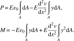
In the above equation, ε0 and the curvature terms are outside the integral because they are a function of the x‐coordinate only. Since the choice of the beam axis (x‐axis) is such that it passes through the centroid of the cross section, the first moment of the area, ![]() , vanishes, and we can recognize the second moment of inertia of the cross section,
, vanishes, and we can recognize the second moment of inertia of the cross section, ![]() , in the expression for bending moment M in the above equation. Now the expressions for P and M take the following forms
, in the expression for bending moment M in the above equation. Now the expressions for P and M take the following forms

where A and I are, respectively, the area and moment of inertia of the cross section. It should be noted that the moment of inertia I is about the z–axis passing through the centroid of the cross section, which is usually denoted by Izz or Iz. The terms EA and EI are called, respectively, the axial rigidity and flexural rigidity of the beam cross section. The first part of eq. (3.6) corresponds to the uniaxial bar in chapter 1. In this section, we will assume the beam does not have any net axial force, that is, ![]() 2. Then from eq. (3.6),
2. Then from eq. (3.6), ![]() . Thus the only equation we need is
. Thus the only equation we need is ![]() . The second part of eq. (3.6) will be called the beam constitutive relation, or the moment–curvature relation. The relationship between the bending moment and the curvature is linear with the proportionality constant of flexural rigidity.
. The second part of eq. (3.6) will be called the beam constitutive relation, or the moment–curvature relation. The relationship between the bending moment and the curvature is linear with the proportionality constant of flexural rigidity.
Since P and M are derived from the stress σxx, their sign conventions are similar to those of stresses rather than those of forces and couples. Positive P, Vy, and M are illustrated in figure 3.2. Note that Vy is the transverse shear force acting on the beam cross section. It is emphasized that these are not externally applied forces or moment; they are internally generated due to the deformation.

Figure 3.2 Positive directions for axial force, shear force, and bending moment of a plane beam
A beam can be subjected to concentrated forces and couples, Fi and Ci, and distributed transverse force p(x) as shown in figure 3.3. These are externally applied loads. Note that F and p are considered positive when they act in the positive y direction, whereas a counterclockwise couple is considered positive. The common units of the distributed force p are N/m and lb/in.

Figure 3.3 Equilibrium of infinitesimal beam section under various loadings
Another set of equations that will complement the moment‐curvature relation of eq. (3.6) are the beam equilibrium equations. Consider the free‐body diagram of the infinitesimal beam shown in figure 3.3. The shear force acting at a cross section is denoted by Vy. Force equilibrium in the y direction requires

or

Similarly, taking moments about z‐axis passing through the right face of the element yields

or

In deriving eqs. (3.7) and (3.8), the term that includes (dx)2 is ignored because it is a higher‐order term. The equations in the boxes in eqs. (3.7) and (3.8) are the equilibrium equations of the beam. Combining these two equations with the beam constitutive relation ![]() , we obtain the governing differential equation of the beam
, we obtain the governing differential equation of the beam

The above equation is a fourth‐order differential equation, and it requires four boundary conditions to determine integral constants.
The stresses in the beam in a cross section can be determined from the bending moment and shear force resultants. The expression for stress σxx in the absence of axial force P can be obtained from eq. (3.3) as
Substituting for the curvature from eq. (3.6) we obtain

Because of the Euler‐Bernoulli beam theory assumptions that ![]() is independent of y and the assumed form of u(x, y) in eq. (3.1), we obtain the shear strain γxy as
is independent of y and the assumed form of u(x, y) in eq. (3.1), we obtain the shear strain γxy as
That is, Euler‐Bernoulli beam theory predicts zero shear strain. However, we know that a beam cross section is subjected to shear stresses, which results in the transverse shear force resultant Vy as derived in eq. (3.8). According to the theory of elasticity, there are nonzero shear strains in a beam, but they are small compared to the normal strains. The average shear stress in a cross section is given by Vy/A, although the maximum shear stress depends on the cross‐sectional geometry. For example, in a rectangular cross section, the shear stress has a parabolic variation through the thickness with maximum value at the center equal to 1.5 times the average shear stress.
We will use the principle of minimum potential energy, the Rayleigh‐Ritz method to be specific, to derive the finite element equations. The potential energy is the net amount of energy that is stored in the structure during its deformation. Referring to chapter 2, the potential energy is defined as
where U is the strain energy, and V is the potential energy of external forces. In the Rayleigh‐Ritz method, the deflection of the beam is expressed in terms of unknown coefficients. The objective is then to represent the potential energy in terms of these coefficients, and then to differentiate it with respect to the coefficients in order to minimize the potential energy.
The energy method requires an expression for strain energy in the beam, which is derived as follows. The strain energy density at a point in the beam is given by

where we have substituted for strain from eq. (3.2) with ![]() . In the context of beams, we define another strain energy density term, which is called the strain energy per unit length of the beam, UL. It is derived by integrating U0 over the entire cross section at a given x:
. In the context of beams, we define another strain energy density term, which is called the strain energy per unit length of the beam, UL. It is derived by integrating U0 over the entire cross section at a given x:

Substituting for U0 from eq. (3.14) in eq. (3.15) yields an expression for strain energy per unit length of the beam

or

The units for UL are J/m or Nm/m or ![]() . By substituting the moment–curvature relation of eq. (3.6) we obtain an expression for UL in terms of M as
. By substituting the moment–curvature relation of eq. (3.6) we obtain an expression for UL in terms of M as ![]() .
.
The strain energy U in the beam can be derived as

Figure 3.3 shows positive directions of concentrated forces, couples, and distributed loads. Using these notations, the potential energy of external forces and moments can be represented by

where NF and NC are, respectively, the number of concentrated forces and couples applied to the beam, and θ(x) is the rotation or slope of the beam.
Thus, the potential energy in eq. (3.13) can be represented using the transverse deflection and slope (derivative of the deflection), as

The principle of minimum potential energy in chapter 2 says that the beam is in equilibrium when the potential energy has its minimum value. We will present the Rayleigh–Ritz method, followed by the finite element method.
3.2 RAYLEIGH‐RITZ METHOD
As discussed in chapter 2, the Rayleigh–Ritz method can be used for continuous systems. In the Rayleigh–Ritz method, a continuous system is approximated as a discrete system with finite number of DOFs. This is accomplished by approximating the displacements by a function containing a finite number of coefficients to be determined. The total potential energy is then evaluated in terms of the unknown coefficients. Then the principle of minimum potential energy is applied to determine the best set of coefficients by minimizing the total potential energy with respect to the coefficients. The solution thus obtained may not be exact. It is the best solution from among the family of solutions that can be obtained from the assumed displacement functions. In the following, we demonstrate the method to beam problems. The steps involved in solving the beam problem using the Rayleigh–Ritz method are as follows.
- Assume a deflection shape for the beam in the following form:
 , where ci are coefficients to be determined, and fi(x) are known bases. The deflection curve
  must satisfy the displacement boundary conditions, for instance, deflection
  or slope
  .
. - Determine the strain energy U in the beam using the formula in eq. (3.17) in terms of ci.
- Find the potential energy of external forces V using formulas of types given in eq. (3.18).
- The total potential energy is obtained as
 .
. - Apply the principle of minimum potential energy to determine the coefficients c1, c2, … cn.

Figure 3.4 Simply supported beam under uniformly distributed load

Figure 3.5 Comparison of finite element results with exact ones for a simply supported beam; (a) deflection, (b) bending moment, and (c) shear force

Figure 3.6 Simply supported beam under a uniformly distributed load
Figure 3.7 Comparison of finite element results with exact ones for a cantilevered beam; (a) deflection, (b) bending moment, and (c) shear force
The Rayleigh‐Ritz method is really a powerful tool to obtain an approximate solution. However, this method has two challenges in order to solve complex problems: (a) it is difficult to find functions that satisfy the displacement boundary conditions, especially when the geometry is complicated; and (b) it is difficult to find functions that can accurately represent the complicated deformation of the entire structure. In the following sections, we develop the finite element version of the Rayleigh‐Ritz method that can resolve these two challenges.
3.3 FINITE ELEMENT FORMULATION FOR BEAMS
3.3.1 Finite Element Interpolation
The finite element method differs from the Rayleigh‐Ritz method in that the approximation is performed within an element, rather than the entire structure. By using the property of interpolation functions, it is trivial to satisfy the essential boundary conditions in this approach. When many elements are used to discretize the structure, simple polynomial‐type functions may be enough to approximate the solution within the element with an acceptable accuracy. In this section, we will present the interpolation method similar to that in chapter 2, but specialized for the beam element. This interpolation will be used in approximating the potential energy in the following section.
Consider a beam shown in figure 3.3. It is subjected to a distributed force and several concentrated or point forces and couples. Our goal is to determine the deflection curve ![]() of the beam, the bending moment distribution M(x), and shear force resultant Vy(x) along the length of the beam. The first step in finite element analysis is to divide the beam into a number of elements. An element is connected to the adjacent element at nodes. Concentrated forces and couples can be applied only at nodes; that means, there should be nodes at points where concentrated forces and couples are applied. In this text, we will consider a beam element that consists of two end nodes. In general, however, it is possible to have more than two nodes in an element. The positive directions of applied forces and couples are shown in figure 3.8. The distributed load p(x) can change along the x‐axis. However, we will only consider the cases of either constant or linear distribution.
of the beam, the bending moment distribution M(x), and shear force resultant Vy(x) along the length of the beam. The first step in finite element analysis is to divide the beam into a number of elements. An element is connected to the adjacent element at nodes. Concentrated forces and couples can be applied only at nodes; that means, there should be nodes at points where concentrated forces and couples are applied. In this text, we will consider a beam element that consists of two end nodes. In general, however, it is possible to have more than two nodes in an element. The positive directions of applied forces and couples are shown in figure 3.8. The distributed load p(x) can change along the x‐axis. However, we will only consider the cases of either constant or linear distribution.

Figure 3.8 Positive directions for forces and couples in a beam element
The DOFs in beam elements are the transverse deflection ![]() and the rotation θ of the cross section that is also equal to the slope
and the rotation θ of the cross section that is also equal to the slope ![]() . The transverse deflection is positive in the positive y direction, whereas a counterclockwise rotation of the cross section is considered positive. Consider a typical element shown in figure 3.9. Our goal is to interpolate the deflection at any point on the element in terms of nodal DOFs
. The transverse deflection is positive in the positive y direction, whereas a counterclockwise rotation of the cross section is considered positive. Consider a typical element shown in figure 3.9. Our goal is to interpolate the deflection at any point on the element in terms of nodal DOFs ![]() . We first define a vector of nodal DOFs, as
. We first define a vector of nodal DOFs, as

Figure 3.9 Nodal displacements and rotations for the beam element
It is convenient to define a parameter s that varies from 0 to 1 within the element so that a unified derivation is possible for an element of any length. The parameter s can be defined as (see figure 3.9)
where x1 is the x‐coordinate of node 1 (first node of the element). Thus, the deflection curve can be written in terms of the parameter s, that is, ![]() 4. The relation in eq. (3.37) can be considered as a mapping between the physical coordinate x and parametric coordinate s. In that regard, the last relation,
4. The relation in eq. (3.37) can be considered as a mapping between the physical coordinate x and parametric coordinate s. In that regard, the last relation, ![]() , is called the Jacobian of the mapping.
, is called the Jacobian of the mapping.
Our goal is to interpolate the deflection ![]() in terms of the nodal DOFs. Since the beam element has four nodal values, it is appropriate to use a cubic function to approximate the deflection with four unknown coefficients:
in terms of the nodal DOFs. Since the beam element has four nodal values, it is appropriate to use a cubic function to approximate the deflection with four unknown coefficients:
where a0, a1, a2, and a3 are the constants to be determined in terms of the nodal DOFs. In addition to the deflection, the slope or rotation θ is also included as the nodal values. Thus, it is necessary to differentiate ![]() with respect to x. However,
with respect to x. However, ![]() in eq. (3.38) is expressed in terms of the parameter s. The expression for the slope can be obtained using the chain rule of differentiation as
in eq. (3.38) is expressed in terms of the parameter s. The expression for the slope can be obtained using the chain rule of differentiation as
Note that the relation ![]() is from eq. (3.37).
is from eq. (3.37).
The expression of the strain energy in eq. (3.16) contains the second derivative of the transverse displacement, whose expression can be obtained by differentiating the above equation as

Now, the four coefficients (a0, a1, a2, and a3) need to be expressed in terms of nodal values. By definition, the vertical displacement at the left end of the element ![]() is
is ![]() , and the slope is θ1. By evaluating eqs. (3.38) and (3.39) at
, and the slope is θ1. By evaluating eqs. (3.38) and (3.39) at ![]() , we can calculate a0 and a1, as
, we can calculate a0 and a1, as

In the same way, we can evaluate (3.38) and (3.39) at ![]() to obtain the following simultaneous system equations, as
to obtain the following simultaneous system equations, as

By solving the above two equations for a2 and a3, we have

Thus, all unknown coefficients are expressed in terms of nodal values. By substituting these coefficients into eq. (3.38), we have

Since our goal is to express ![]() in terms of nodal values, eq. (3.41) can be rearranged to obtain
in terms of nodal values, eq. (3.41) can be rearranged to obtain

An important concept in finite element approximation is the definition of the shape functions, which are the coefficients of the nodal values. The deflection ![]() in (3.42) can be written in the form
in (3.42) can be written in the form ![]() . The coefficients of the nodal DOFs in eq. (3.42) are called the shape functions of the beam element:
. The coefficients of the nodal DOFs in eq. (3.42) are called the shape functions of the beam element:

Equation (3.41) can then be written in matrix form as

or
where {N} is the column vector of shape functions of the beam element. Equation (3.44) approximates the deflection of the beam using the values of deflections and slope at the two nodes. For example, evaluation of eq. (3.44) at ![]() will provide the beam deflection at the center of the element.
will provide the beam deflection at the center of the element.
Figure 3.10 shows the plot of the shape functions. These shape functions are also called the Hermite polynomials. Note that when ![]() , all shape functions are zero except for N1, which is equal to unity. Thus, eq. (3.41) yields
, all shape functions are zero except for N1, which is equal to unity. Thus, eq. (3.41) yields ![]() , which is the desired result. When
, which is the desired result. When ![]() , the only nonzero shape function is N3. Thus, the approximation in eq. (3.41) yields
, the only nonzero shape function is N3. Thus, the approximation in eq. (3.41) yields ![]() .
.

Figure 3.10 Shape functions of the beam element
Note that the interpolation of the beam deflection in eq. (3.44) is valid within an element. If the beam consists of more than one element, the interpolation must be performed in each element. Two adjacent elements will have continuous deflection and slope, as they share the nodal values.
The second derivative of the deflection in eq. (3.40) can be derived as

or

where the column vector {B} is, in general, called the strain–displacement vector. In the context of beams, it relates the curvature of the beam to the nodal displacements. Note that the vector {B} is a linear function of the parameter s. Thus, the curvature varies in a linear fashion within an element. The reader can verify that the curvature term in (3.45) can also be written as
Equation (3.45) provides some information about the quality of interpolation. If the loads acting on a beam results in a constant or linear variation of curvature or bending moment, then the interpolation in eq. (3.45) will represent it accurately. However, when a problem requires a higher‐order variation of curvature (bending moment) with respect to x, then the interpolation is only an approximation. In such a case, several beam elements will be required to approximate the higher‐order variation of the bending moment with a reasonable accuracy.
Using eq. (3.45), the bending moment and shear force in the beam element can also be calculated in terms of nodal DOFs, as
It is interesting to note that the bending moment is a linear function of s, and thus, x, while the shear force is constant throughout the element. This is because the assumed deflection is a cubic function as in eq. (3.38). Since the stress is proportional to the bending moment as shown in eq. (3.11), the maximum stress occurs at the location of the maximum bending moment. Since the bending moment varies linearly, the maximum stress always occurs at either nodes of the beam element. However, caution is required because the bending moments between two adjacent elements are discontinuous at the node.
Equation (3.45) can be used to approximate the strain energy in the following section.

Figure 3.11 Cantilevered beam element with nodal displacements
3.3.2 Finite Element Equation for the Beam Element
As the reader may recall, one of the steps in finite element analysis is to express the strain energy of the solid in terms of nodal DOFs. In this section, we will derive the finite element equation using the principle of minimum potential energy. Let us consider a beam, shown in figure 3.12, with the total length of LT. The beam is divided into NEL number of beam elements with equal length L. The elements do not have to be of the same length, but the assumption makes the explanation simple. We further assume that the cross‐sectional area remains constant within an element. The beam is under concentrated forces and couples at the nodes and distributed load p(x).

Figure 3.12 Finite element models using four beam elements
The strain energy in a beam can be formally written in terms of strain energy per unit length as

where U(e) is the strain energy of element e. The integration is performed over each beam element and summed over NEL number of elements. Note that ![]() and
and ![]() , respectively, are the x‐coordinates of the first and second nodes of element e. Substituting for UL from eq. (3.16) we obtain
, respectively, are the x‐coordinates of the first and second nodes of element e. Substituting for UL from eq. (3.16) we obtain

In the above equation, we have used the relation ![]() ; see eq. (3.37). The expression of the strain energy in eq. (3.50) contains the second‐order derivative of deflection
; see eq. (3.37). The expression of the strain energy in eq. (3.50) contains the second‐order derivative of deflection ![]() . Using the interpolation in eqs. (3.45) and (3.46), we can write the second‐order derivative term as
. Using the interpolation in eqs. (3.45) and (3.46), we can write the second‐order derivative term as

Note that for the first curvature term, we have used {q}T{B}, and for the second, {B}T{q}. Substituting the above relation in eq. (3.50), the strain energy of element e is derived as

where [k(e)] is the element stiffness matrix of the beam finite element. After integrating, the stiffness matrix can be derived as

or

which is a symmetric 4 × 4 matrix. Note that the element stiffness matrix is proportional to the flexural rigidity EI and inversely proportional to L3. The stiffness matrices of all the elements can then be calculated from the element properties. The strain energy in the beam can then be obtained by summing strain energies of the individual elements as in eq. (3.49):

or

where {Qs} is the column matrix of all DOFs in the beam, and [Ks] is the structural stiffness matrix obtained by assembling the element stiffness matrices. The assembly procedure, which is similar to that of a uniaxial bar and truss elements, will be illustrated in the examples to follow.

Figure 3.13 Finite element models of stepped cantilevered beam
The next step is to derive an expression for the potential energy of external forces. If there are only concentrated forces and couples acting on the beam, the potential energy V can be written as

where Fi and Ci, respectively, are the transverse force and couple acting at node i, and the total number of nodes in the beam model is denoted by ND. The above expression for V can be written in a matrix form as
where {Fs} is the vector of nodal forces.
If there are distributed forces acting on the beam, then they have to be converted into equivalent nodal forces. Let us assume that the distributed load acting on the beam is given by p(x). Then the potential energy of this load is given by

where LT is the total length of the beam. The integral can be broken down to integrals over each element as

In the above equation, V(e) is the contribution to V by element e, which can be derived as

In the above equation, p(s) should be expressed as a function of s using the change of variables given by eq. (3.37). Now we will use the shape functions to express ![]() within an element in terms of nodal displacements using eq. (3.44) to obtain
within an element in terms of nodal displacements using eq. (3.44) to obtain

The terms inside the parentheses in the above equation are called work equivalent loads contributed by element e and are denoted by ![]() . These loads can be calculated from the distributed load p, the shape functions, and element length L. One can note that a transverse load p results not only in two concentrated forces at the nodes but also results in couples acting at the nodes. If a node belongs to more than one element, then the contributions from all elements at that node must be added together along with any applied concentrated forces and couples.
. These loads can be calculated from the distributed load p, the shape functions, and element length L. One can note that a transverse load p results not only in two concentrated forces at the nodes but also results in couples acting at the nodes. If a node belongs to more than one element, then the contributions from all elements at that node must be added together along with any applied concentrated forces and couples.

Figure 3.14 Work equivalent nodal forces for the distributed load
Using the strain energy in eq. (3.53) and the potential energy of the applied loads in eq. (3.55), the total potential energy of the beam can be written as
The principle of minimum potential energy can be applied to determine the unknown DOFs {Qs}. One can recognize Π above as a quadratic function in {Qs}. Using the minimization principle derived in section A.6 of the appendix for a quadratic form, the stationary condition of Π with respect to {Qs} yields
The above equations are the structural equations for the beam. In general, the structural stiffness matrix [Ks] will be singular. We can apply the boundary conditions by deleting the rows and columns corresponding to zero DOFs to obtain the global matrix equation as
This process is the same with that of the truss elements in chapter 1. The only difference is that the boundary conditions include not only the displacement but also the slope or rotation of the beam.

Figure 3.15 Finite element models of stepped cantilevered beam

Figure 3.16 Cantilevered beam under uniformly distributed load and couple

Figure 3.17 Comparison of beam deflection and rotation with exact solutions; (a) deflection, (b) slope
3.3.3 Bending Moment and Shear Force Distribution
After the nodal DOFs are determined, the bending moment M(s) and shear force Vy(s) distribution along the element can be calculated by substituting for the deflection curve into eqs. (3.6) and (3.8).
Bending moment:
Shear force:

Note that the moment is a linear function of s, while the shear force is constant in an element. This is a limitation of the current beam element. If the loads on the beam are such that the shear force has a linear distribution, then several elements must be used so that the linear variation of the shear force can be better approximated by the piecewise constant shear force distribution.
We can use eq. (3.65) to calculate the bending moment at the two nodes of the beam element. We will denote the bending moments at nodes 1 and 2 by M1 and M2, respectively. They can be calculated as


From eqs. (3.66) through (3.68), we can write the shear force and bending moments at the two nodes in a matrix form as shown below:

One can note that the square matrix in the above equation is identical to the stiffness matrix of the beam element [see eq. (3.52)].
After calculating the bending moment, the axial stress in the beam at a cross section is calculated using:
It is clear that the maximum stress appears either at the top or bottom of the beam element, which corresponds to ![]() where the beam height is h.
where the beam height is h.
The computation of the shear stress is more complicated and depends on the shape of the cross section. For a rectangular section of width b and height h, the shear stress distribution is given by

The maximum shear stress appears at the neutral axis of the beam ![]() , and it is zero at the top and bottom of the cross section. The maximum shear stress is 1.5 times the average shear stress, which is equal to Vy/bh.
, and it is zero at the top and bottom of the cross section. The maximum shear stress is 1.5 times the average shear stress, which is equal to Vy/bh.

Figure 3.18 Comparison of bending moment and shear force with exact solutions; (a) bending moment, (b) shear force

Figure 3.19 One element model with distributed force p

Figure 3.20 Transverse displacement of the beam element

Figure 3.21 Comparison of FE and analytical solutions for the beam shown in figure 3.19; (a) bending moment, (b) shear force
3.4 PLANE FRAME ELEMENTS
Even if a beam element in the previous section can be useful, it is often not enough to model many practical applications. For example, each member of the portal frame in figure 3.22 needs to support not only transverse shear and bending moment but also axial load. That is, a structural member can play the role of both uniaxial bar and beam at the same time. Therefore, it would be necessary to combine the bar and beam elements for practical engineering applications.
3.4.1 Plane Frame Element Formulation
A plane frame is a structure similar to a truss, except the members can carry a transverse shear force and bending moment in addition to an axial force. Thus, a frame member combines the action of a uniaxial bar and a beam. This is accomplished by connecting the members by a rigid joint such as a gusset plate, which transmits the shear force and bending moment. Welding the ends of the members will also be sufficient in some cases. The cross sections of members connected to a joint (node) undergo the same rotation when the frame deforms. The nodes in a plane frame, which is in the x‐y plane, have three DOFs, u, v, and θ, displacements in the x and y directions, and rotation about the z‐axis. Consequently, one can apply two forces and one couple at each node corresponding to the three DOFs. An example of common frame is depicted in figure 3.22.

Figure 3.22 Frame structure and finite elements
Consider the free‐body diagram of a typical frame element shown in figure 3.23. It has two nodes and three DOFs at each node. Each element has a local coordinate system. The local or element coordinate system ![]() is such that the
is such that the ![]() ‐axis is parallel to the element. The positive
‐axis is parallel to the element. The positive ![]() direction is from the first node to the second node of the element. The
direction is from the first node to the second node of the element. The ![]() ‐axis is such that the
‐axis is such that the ![]() ‐axis is in the same direction as the z‐axis. In the local coordinate system, the displacements in
‐axis is in the same direction as the z‐axis. In the local coordinate system, the displacements in ![]() and
and ![]() directions are, respectively, ū and
directions are, respectively, ū and ![]() , and the rotation in the
, and the rotation in the ![]() direction is
direction is ![]() . Each node has these three DOFs. The forces acting on the element, in local coordinates, are
. Each node has these three DOFs. The forces acting on the element, in local coordinates, are ![]() at node 1, and
at node 1, and ![]() at node 2. Our goal is to derive a relation between the six element forces and the six DOFs. It will be convenient to use the local coordinate system to derive the force–displacement relation as the axial effects and bending effects are uncoupled in the local coordinates.
at node 2. Our goal is to derive a relation between the six element forces and the six DOFs. It will be convenient to use the local coordinate system to derive the force–displacement relation as the axial effects and bending effects are uncoupled in the local coordinates.

Figure 3.23 Local degrees of freedom of plane frame element
The element forces and nodal displacements are vectors, and they can be transformed to the ![]() coordinate system as follows:
coordinate system as follows:

or
where the transformation matrix [T] is a function of the direction cosines of the element. Note that the size of the transformation matrix [T] in chapter 1 was 4 × 4, as a two‐dimensional truss element has four DOFs. The transformation matrix in eq. (3.76) is basically the same, but the size is increased to 6 × 6 because of additional couples. However, the couple ![]() is the same as the couple c, as the local
is the same as the couple c, as the local ![]() ‐axis is parallel to the global z‐axis. For the same reason,
‐axis is parallel to the global z‐axis. For the same reason, ![]() . Since the displacements are also vectors, a similar relation connects the DOFs in the local and global coordinates:
. Since the displacements are also vectors, a similar relation connects the DOFs in the local and global coordinates:

or
In the local coordinate system, the axial deformation (uniaxial bar) and bending deformations (beam) are assumed uncoupled. When the beam is bent significantly, the axial load can affect the bending moment. Therefore, this assumption requires that bending deformation is infinitesimally small, which is the basic assumption in linear beam theory. Under such assumption, the axial forces and axial displacements are related by the uniaxial bar stiffness matrix, as

On the other hand, the transverse force and couple are related to the transverse displacement and rotation by the bending stiffness matrix in eq. (3.52), as

In a sense, the plane frame element is a combination of two‐dimensional truss and beam elements. Combining eqs. (3.78) and (3.79), we obtain a relation between the element DOFs and forces in the local coordinate system:

where
It is clear that the equations at the first and fourth rows are the same as the uniaxial bar relation in eq. (3.78), whereas the remaining four equations are the beam relation. Equation (3.80) can be written in symbolic notation as
where ![]() is the element stiffness matrix in the local coordinate system.
is the element stiffness matrix in the local coordinate system.
As in the case of two‐dimensional truss elements, the element matrix equation (3.81) cannot be used for assembly because different elements have different local coordinate systems. Thus, the element matrix equation needs to be transformed to the global coordinate system. Substituting for ![]() from eqs. (3.76) and (3.77), we obtain
from eqs. (3.76) and (3.77), we obtain
Multiplying both sides of the above equation by ![]() , we obtain
, we obtain
It can be shown that for the transformation matrix ![]() . Hence, eq. (3.83) can be written as
. Hence, eq. (3.83) can be written as
or
where ![]() is the element stiffness matrix of a plane frame element in the global coordinate system. One can verify that [k] is symmetric and positive semi‐definite.
is the element stiffness matrix of a plane frame element in the global coordinate system. One can verify that [k] is symmetric and positive semi‐definite.
Assembly of the element stiffness matrix to form the structural stiffness matrix [Ks] follows the same steps as for earlier elements. After deleting the rows and columns corresponding to zero DOFs, we obtain the global equations in the form ![]() .
.
3.4.2 Calculation of Element Forces
After solving the global equations, the DOFs of all elements are known in the frame structure. Let us represent the DOF of a typical element by {q} which is a 6 × 1 column matrix. We will transform the DOFs into local coordinates using eq. (3.77) to obtain ![]() . Then, the axial force in the element can be obtained using
. Then, the axial force in the element can be obtained using
This relation is exactly the same as that of a uniaxial bar element. We note that the transverse shear force is constant throughout the element, and the bending moment varies linearly. Thus, it is enough to find the nodal values. From eq. (3.69), the nodal values of bending moments and shear forces can be found by


Figure 3.24 A two‐member plane frame

Figure 3.25 Deformed shape of the frame in figure 3.24. The displacements are magnified by a factor of 200
Force and moment resultants: We will use eq. (3.81), ![]() , to obtain the force and moment resultants. Consider element 1 first. We already know the element stiffness matrix
, to obtain the force and moment resultants. Consider element 1 first. We already know the element stiffness matrix ![]() and the displacements
and the displacements ![]() for this element. Performing the matrix multiplication, we obtain the forces as:
for this element. Performing the matrix multiplication, we obtain the forces as:
From the above result one can recognize the axial force P, shear force V, and moment resultants M1 and M2 in element 1 as:

The above forces are shown in the free‐body diagram of element 1 in figure 3.26. Note the orientation of the local ![]() coordinate system. Force resultants P and V are constant along the length of the element. The bending moment varies linearly from M1 at node 1 to M2 at node 1.
coordinate system. Force resultants P and V are constant along the length of the element. The bending moment varies linearly from M1 at node 1 to M2 at node 1.
The forces in element 2 were calculated using similar procedures to obtain:

Note that nodes 2 and 3 were the first and second nodes for element 2. The free‐body diagram of element 2 is shown in figure 3.26 along with that of element 1.

Figure 3.26 Free‐body diagrams of elements 1 and 2 of the frame in example 3.10
Support Reactions The reactions at node 1 are basically given by ![]() (N‐m units). Similarly reactions at node 3 are:
(N‐m units). Similarly reactions at node 3 are: ![]() . But they are in respective local coordinate systems. They have to be resolved into the global x‐y coordinates as shown in figure 3.27. Checking for global equilibrium is left to the student as an exercise in statics. Note there are roundoff errors in the reactions shown.
. But they are in respective local coordinate systems. They have to be resolved into the global x‐y coordinates as shown in figure 3.27. Checking for global equilibrium is left to the student as an exercise in statics. Note there are roundoff errors in the reactions shown.

Figure 3.27 Support reactions for the frame in example 3.10
3.5 BUCKLING OF BEAMS
In engineering structures, buckling is instability that leads to a failure mode. It happens when the structure or elements within the structure are subjected to a compressive load or stress, especially when the structure has slender members such as a beam. For example, an eccentric compressive axial load may cause a small initial bending deformation to the beam. However, the bending deformation increases the eccentricity of the load and thus further bends the beam. This can possibly lead to a complete loss of the member’s load‐carrying capacity. Buckling may occur even though the stresses that develop in the structure are well below the failure strength of the material. Therefore, buckling is an important failure mode, and engineers should be aware of it when designing structures.
3.5.1 Review of Column Buckling
Consider a cantilevered beam subjected to an end couple C and an axial force P (figure 3.28). We are interested in the tip deflection of the beam. If we use the concept of linear superposition for elastic structures (see section 1.3.3), then the axial force P should have no effect on the flexural behavior due to the couple C, and the tip deflection should be equal to CL2/2EI. However, the engineering sense tells us that it should be difficult for the couple to bend the beam because the axial force is trying to straighten the beam. That is, the deflection of the beam should be less because of the axial force P. The opposite will be true if the axial force were compressive, that is, the deflection will be larger, because a compressive axial force will tend to aid the couple in bending the beam. The effect of the axial force can be easily understood, if we look at the free‐body diagram of the beam in figure 3.29 and compute the bending moment at a cross section at a distance x.

Figure 3.28 A beam subjected to axial force and an end couple

Figure 3.29 Beam subjected to an axial tension and an end couple with a free‐body diagram to determine M(x)
The bending moment at x is given by
where v(x) is the beam deflection, and δ is the tip deflection. In elementary beam theory, we do not consider the second term on the right‐hand side of eq. (3.95) as it is assumed small compared to the applied couple C because either P is small or the deflection δ is small. This is the fundamental assumption for linear problems, and we used this assumption when we derive the equation for the frame element. From the constitutive relations of the beam [see eq. (3.6)], we know the curvature of the beam is proportional to the bending moment:
By substituting eq. (3.96) in eq. (3.95), we obtain
Equation (3.97) is an ordinary differential equation, whose solution consists of complementary functions and a particular integral given by:

where A and B are constants to be determined from the boundary conditions, and the parameter λ is given by
The boundary conditions are similar to the cantilever beam such that at x = 0, deflection v and slope ![]() are equal to zero. Substituting the boundary conditions in eq. (3.98) and solving for A and B, we obtain the final solution as
are equal to zero. Substituting the boundary conditions in eq. (3.98) and solving for A and B, we obtain the final solution as

The tip deflection δ can be found by using δ = v(L) in eq. (3.100):

It can be seen from eq. (3.101) that the effect of axial tension P is to reduce the tip deflection. As P → ∞, λ → ∞ and δ → 0. When P → 0, λ → 0, and the tip deflection approaches the beam theory deflection CL2/2EI. Evaluation of this limit is left to the reader as an exercise in calculus.
If the force P is compressive, a similar procedure can be used to find the deflection v(x). The only change will be in the sign of P in eq. (3.99). Since P is negative for a compressive load, the parameter λ becomes imaginary. This will lead to sin and cos terms in the solution instead of sinh and cosh terms. The solution after applying the boundary conditions can be derived as

Solving for delta using v(L) = δ, we obtain

Again, one can show that as P → 0 from the negative side, the tip deflection approaches the beam theory deflection CL2/2EI. One can note that the tip deflection will become unbounded when λL → π/2. This corresponds to an axial compressive force given by

where Pcr is called the critical load for buckling of the beam. One can note that Pcr does not depend on the external couple C that is applied but depends only on the flexural rigidity EI of the cross section and the beam length L. Thus, it is a structural property. When the axial load is tensile, the beam apparently becomes stiff, and this phenomenon is called stress stiffening. The effect of compressive axial load is called stress softening.
3.5.2 End Shortening Due to Compressive Load
In the previous section, we solved the differential equation of the beam to understand the effect of axial forces on the beam flexural behavior. In applying energy methods, we need to identify the additional energy terms due to coupling of P and the flexural deformation. We achieve this by accounting for the axial displacement of the beam due to bending. Let us assume that the axial rigidity of the beam, EA, is infinitely large. Then, the beam neutral surface does not undergo any stretching. From figure 3.30, one can note that as the beam undergoes a large deflection, the point of application of load P moves inwards in order to keep the beam length constant. Thus, the force P moves through a distance Δ as shown in the figure. That means there is a work performed by P. We have to add a corresponding term in the expression for the total potential energy. The end shortening Δ depends only on the beam deflection, and its derivation is given below.

Figure 3.30 End shortening of a cantilever beam under a compressive load
Consider the deformation of an infinitesimal length dx of the beam depicted in figure 3.30. The relative axial displacement of the two ends of this element can be derived as:
where θ is the rotation of the element. When the rotational angle is small, it can be approximated by ![]() . Therefore, we obtain
. Therefore, we obtain

The total axial displacement or the end shortening of the beam is obtained by integrating the differential end shortening to the entire beam, as

3.5.3 Rayleigh‐Ritz Method
Consider the example given at the beginning of this section (i.e., figure 3.28). Let us assume the axial force P is tensile. We will solve this problem using the Rayleigh‐Ritz method. First, the deflection of the beam is approximated as:
which satisfies all kinematic boundary conditions at x = 0. The strain energy U in the beam can be computed in terms of c as [see eq. (3.17)]

The next step is to express the potential energy of external forces in terms of c. If we use the small deflection theory, only the couple C would contribute to this term. However, in the present situation we need to account for the potential of the axial force P also. The energy term V can be expressed as

In the above equation, Δ has a negative sign because the beam end is moving in the negative x direction (end shortening), whereas the force P is in the positive direction. Substituting for Δ from eq. (3.106) and for v(x) from eq. (3.107), we obtain

Now the total potential energy can be written as
The equilibrium of the structure occurs when the total potential energy is stationary in the Rayleigh‐Ritz method. Since the only unknown variable is the coefficient c, the derivative of the total potential energy with respect to c has to be zero:

Therefore, the beam deflection curve can be obtained using eq. (3.107). Using the same equation, the maximum deflection at the tip is given by

From eq. (3.113) one can note that a tensile P will decrease the maximum deflection δ. The expression in eq. (3.113) can be used even if P < 0 by changing the sign of P. Then

From eq. (3.114) one can derive the approximate Pcr at which the deflection becomes unbounded by equating the denominator to zero:
We note that the value of Pcr obtained by using the Rayleigh‐Ritz method is about 20% larger than the exact buckling load for a cantilevered beam, which is given by ![]() in eq. (3.104). This is typical of approximate methods, as they tend to make the structure look stiffer.
in eq. (3.104). This is typical of approximate methods, as they tend to make the structure look stiffer.
The above results can be non‐dimensionalized by dividing by the tip deflection of a beam:

The exact solution obtained in eqs. (3.101) and (3.103) can be written in non‐dimensional forms as

The non‐dimensional tip deflections are plotted as a function of the non‐dimensional load term λL in figure 3.31. For the case of compressive axial load ![]() , one can note that the non‐dimensional tip deflection will become unbounded when
, one can note that the non‐dimensional tip deflection will become unbounded when ![]() for the exact solution in eq. (3.117) and when
for the exact solution in eq. (3.117) and when ![]() for the approximate solution given by eq. (3.116).
for the approximate solution given by eq. (3.116).

Figure 3.31 Non‐dimensional tip deflection as a function of non‐dimensional axial force λL for a given end couple in a cantilever beam
3.5.4 Finite Element Method for Buckling of Beams
The finite element formulation of buckling or stress stiffening follows a similar procedure as in the Rayleigh‐Ritz method. The beam element discussed earlier can be modified for buckling analysis. Basically we divide the beam into a number of elements. Each element has two nodes, and each node has two DOFs, the transverse deflection v and rotation or slope θ. We assume that the axial force P is constant in each element. Then the potential energy of these forces can be given as [see eq. (3.109)]

where Vinc denotes the potential energy of P, P(e) is the axial force in element e, Δ(e) is the axial shortening of node j with respect to node i of element e, and NEL is the total number of elements. The subscript “inc” in Vinc refers to incremental energy because this is an additional energy as the beam undergoes large deflections. In fact, it will be shown later that Vinc will increase the stiffness for stress stiffening or decrease for buckling. The displacement Δ(e) is the end‐shortening of element e and is derived as:

where xi and xj are respectively the x‐coordinates of the first and second nodes of the element e.
Before we proceed further, the sign conventions used herein are worth discussing. One may note the usual negative sign in the expression for potential is energy missing in eq. (3.118). In the derivation of potential energy, the axial force P is taken as tensile and hence positive. The term Δ(e) is end shortening and hence is negative, which cancels the negative sign in the expression for potential energy.
By using the change of variable ![]() as defined in eq. (3.37), we obtain
as defined in eq. (3.37), we obtain

The derivative dv/ds can be written in terms of the nodal DOFs and the shape functions Ni(s) as

In the above equation, a prime (′) denotes the first derivative dN/ds with respect to s. The shape functions are given in eq. (3.43).
Substituting from (3.121) into (3.120) yields
where {q} is the column vector of element DOFs, and the components of symmetric incremental stiffness matrix ![]() can be calculated using the following formula:
can be calculated using the following formula:

After substituting four shape functions, ![]() can be obtained as
can be obtained as

The row addresses of ![]() are shown next to the matrix in eq. (3.124).
are shown next to the matrix in eq. (3.124).
Substituting for Δ(e) from eq. (3.122) into eq. (3.118), the expression for Vinc is obtained as

In general P(e) will be different in different elements, and hence it cannot be factored when assembling the incremental stiffness matrices. We will multiply and divide by a reference load Pr as shown below:

where [PrKinc] is the global incremental stiffness matrix obtained by assembling ![]() and {Q} is the column vector of active DOFs. The total potential energy of the beam can be written as
and {Q} is the column vector of active DOFs. The total potential energy of the beam can be written as

From eq. (3.127), one can see why [Kinc] is called the incremental stiffness matrix. The effect of axial tension is to add a positive definite matrix to the stiffness matrix, thus increasing the strain energy of the system, which makes the beam stiffer. By the same token, if the axial forces are negative (compressive), the beam will appear softer or more compliant. Minimization of Π with respect to {Q} leads to the following standard finite element system of equations:
where [KT] is the total stiffness matrix. If the inverse for [KT] exists, then one can find it and determine the displacements {Q} for a given set of transverse forces and couples {F} acting on the beam. This will be the case when the beam is stable and the displacement {Q} determines the static deformation. The only difference from the previous beam analysis in section 3.3 is that the bending and axial deformation are coupled. The incremental stiffness matrix in eq. (3.124) has a constant of 1/30 L, while the beam stiffness matrix in eq. (3.52) has a constant of EI/L3. Therefore, if the condition of 1/30 L < < EI/L3 is satisfied, then it is possible to ignore the effect of incremental stiffness, which is the case in the beam formulation in section 3.3. However, this is not the main interest in this section, where we look for a case when the effect of the incremental stiffness is significant.
If the axial forces P are such that the determinant of [KT] is equal to zero, then it cannot be inverted, and the deflections {Q} are undefined. In physical terms, the deflections can become unbounded. Values of Pr that satisfy this condition are the critical loads (Pcr) for buckling of the beam, and they are solved using the polynomial equation for Pr obtained from
Usually we are concerned with the first or the lowest Pcr because the applied load increases gradually from zero. When the axial load reaches Pcr, the beam will buckle and collapse. Even if the zero‐determinant equation in eq. (3.129) looks independent of the applied loads, it actually depends on the applied load because the element force is required in the form of ![]() in the assembly of the incremental stiffness matrix. Therefore, when solving for buckling loads, the static analysis is solved first without considering buckling to calculate element forces, and then, eq. (3.129) is solved for the buckling loads. In fact, eq. (3.129) is the necessary condition for following the generalized eigenvalue problem (see eq. (A.66) in appendix):
in the assembly of the incremental stiffness matrix. Therefore, when solving for buckling loads, the static analysis is solved first without considering buckling to calculate element forces, and then, eq. (3.129) is solved for the buckling loads. In fact, eq. (3.129) is the necessary condition for following the generalized eigenvalue problem (see eq. (A.66) in appendix):
where Pr is the eigenvalue and {Q} is corresponding eigenvector. The eigenvectors for each eigenvalue define the corresponding mode shape or shape of the buckled beam. This will be illustrated in the following examples.

Figure 3.32 Deflection curve of a cantilever beam subjected to an end couple and different values of the axial force P
![Graph of v(x) [m] vs. x [m] displaying three ascending curves representing v (P = 0) (solid), v (P = +2000 N) (dashed), and v (P = –2000 N) (dash-dotted).](http://images-20200215.ebookreading.net/2/1/1/9781119078722/9781119078722__introduction-to-finite__9781119078722__images__c03f033.gif)
Figure 3.33 Buckling mode shapes of a cantilever beam obtained using one beam finite element
![Graph of v(x) vs. x [m] for buckling mode shapes of a cantilever beam obtained using one beam finite element, displaying solid and dashed curves representing mode 1 and mode 2, respectively.](http://images-20200215.ebookreading.net/2/1/1/9781119078722/9781119078722__introduction-to-finite__9781119078722__images__c03f034.gif)
Figure 3.34 Clamped‐hinged beam subjected to an axial force

Figure 3.35 Buckling mode shapes for the beam in example 3.13 with two elements
3.6 BUCKLING OF FRAMES
Buckling analysis of plane frames follows essentially the same steps as buckling of beams. The stiffness matrix of a frame element was derived in section 3.4; for example, see eq. (3.80). For plane frames, each node has three DOFs, u, v, and θ. In deriving the stiffness matrix, we combined the stiffness matrices of a beam element and a uniaxial bar element. We will follow a similar procedure for deriving the incremental stiffness matrix [kinc] also. It is noted that in the calculation of the stiffness matrix in eq. (3.80), we assumed that bending and tension are decoupled. On the other hand, in the derivation of buckling of the beam in section 3.5, it is assumed that the axial tension or compression can affect the bending deformation. However, the outcome of buckling analysis is the incremental stiffness matrix, which is solely a function of geometry. Therefore, it is still reasonable to assume that the bending and tension are decoupled in the calculation of the plane frame elements.
Consider a generic frame element shown in figure 3.36.

Figure 3.36 Degrees of freedom of plane portal frame
This is similar to the one in figure 3.23 except an axial compressive force P(e) is acting on the element. The axial force can be determined by a static analysis of the frame as described in section 3.4. The element stiffness matrix in the local ![]() coordinate system is given in eq. (3.80). The incremental stiffness matrix of the frame element in local coordinates will be similar to that of a beam element in eq. (3.124) except extra zeros are added for the axial DOFs ū1 and ū2:
coordinate system is given in eq. (3.80). The incremental stiffness matrix of the frame element in local coordinates will be similar to that of a beam element in eq. (3.124) except extra zeros are added for the axial DOFs ū1 and ū2:

The above incremental stiffness matrix is transformed to global coordinates using the transformation in the same way as the stiffness matrix is transformed by ![]() (see section 3.4):
(see section 3.4):
Then the incremental stiffness matrices of various elements are assembled to obtain the global incremental stiffness matrix [PrKinc] as shown in eq. (3.126).

Figure 3.37 A portal frame subjected to two axial forces

Figure 3.38 First mode (assymteric or swaying mode) and second mode (symmteric mode) buckling of the portal frame in example 3.14
3.7 FINITE ELEMENT MODELING PRACTICE FOR BEAMS
In this section, several analysis problems are used to discuss modeling issues as well as verifying the accuracy of the analysis results by comparing with literature. The examples are presented in such a way that any finite element analysis program can be used to solve the problems. However, the analysis results can be slightly different because of implementation differences between the finite element analysis programs.
3.7.1 Stress and Deflection Analysis of a Beam6
A standard 30 in. wide‐flange beam, with a cross‐sectional area A = 50.65 in2 and the second moment of inertia Iz = 7892 in4 is supported as shown in figure 3.39. A uniformly distributed load w = 10,000 lb/ft is applied on the two overhangs. Determine the maximum bending stress σ and the deflection δ at the middle portion of the beam. Use E = 3.0 × 10⁷ psi. L = 20 ft, a = 10 ft, h = 30 in.

Figure 3.39 Beam bending with distributed loads
In order to solve for the stress and deflection, it is necessary to calculate the bending moment in the beam. Due to symmetry in geometry and loading, the portion between two supports will have a constant bending moment. From the moment equilibrium, the bending moment in the middle portion can be calculated as
Since the above bending moment is constant, stress will also be constant in the middle portion. At the top of the beam cross‐section, the maximum stress can be calculated as

In order to calculate the deflection in the middle portion, the relation between bending moment and curvature ![]() can be used. For this purpose, let us assume that the origin is located at the left support. Since M is constant,
can be used. For this purpose, let us assume that the origin is located at the left support. Since M is constant, ![]() is also a constant; that is, the deflection curve is a quadratic function:
is also a constant; that is, the deflection curve is a quadratic function: ![]() . Using the boundary conditions,
. Using the boundary conditions, ![]() , the following form of deflection curve can be obtained:
, the following form of deflection curve can be obtained:
The unknown coefficient can be calculated from the relation ![]() ,
,
The maximum deflection occurs at the center of the middle portion at x = 10 ft,
For finite element modeling, it is enough to use a single element in the middle portion because the bending moment is constant. However, since the stress and deflection at the center of the middle portion is of interest, two beam elements can be used. Including the two overhangs, a total of four equal‐length beam elements are used to model the problem, as shown in figure 3.39.
The distributed load in the overhangs is constant in the negative y‐coordinate direction. Different finite element analysis programs use different ways of applying distributed loads on a beam. The uniformly distributed load is the simplest one, and many programs allow to input a functional form of distributed load. Note that the distributed load is a force per unit length, not force per unit area.
In the case of a bar or truss, only the cross‐sectional area is required to calculate stress. However, in the case of beam, the cross‐sectional geometry is important as it affects the moment of inertia as well as stress calculation. Therefore, it is required to input cross‐sectional geometry. Many finite element programs support a functionality of defining various cross‐sectional geometries, such as circular, rectangular, hollow‐cylinder, I‐section, and so forth. As shown in figure 3.39, an I‐section beam is used for this example.
The following table shows nodal displacements and rotations of the beam. As expected, the deformation is symmetric with respect to the center. A very small rotation θ = 0.24395E‐17 is calculated for node 3, but this is due to numerical error. Compared to other rotations, this can be considered as zero.
| Node | v | θ |
| 1 | −0.48274 | 0.40547E‐02 |
| 2 | 0.0 | 0.30411E‐02 |
| 3 | 0.18246 | 0.24395E‐17 |
| 4 | 0.0 | −0.30411E‐02 |
| 5 | −0.48274 | −0.40547E‐02 |
Using the nodal displacements and rotations in the above table, the deflection curve of the beam can be obtained using the beam shape functions in eq. (3.43). Figure 3.40 shows the deflection curve of the beam. As expected, the deflections at nodes 2 and 4 are zero, and the maximum occurs at node 3.

Figure 3.40 Deflection curve of the beam
In order to calculate stress, the bending moment should be calculated first. In element 2, the bending moment can be calculated from eq. (3.47) as
Note that the bending moment is constant in the element, and its value is identical to the analytical solution. Therefore, the stress will be the same as the analytical solution. The finite element solution happens to be accurate because the true deflection is a quadratic polynomial and the finite element shape functions are cubic polynomials.
3.7.2 Portal Frame Under Symmetric Loading7
A portal frame with I‐beam sections is subjected to a uniformly distributed load ω = 500 lb/in across the span as shown in figure 3.41. The length of the span is L = 800 in., while the height of the column is a = 400 in. The objective is to determine the maximum rotation and maximum bending moment. The moment of inertia for the span, Ispan is five times the moment of inertia for the columns, Icol; Icol = 20,300 in4 and Ispan = 101,500 in4. For material properties, Young’s modulus E = 30 × 106 psi and Poisson’s ratio ν = 0.3.
All the members of the frame are modeled using I‐beam cross sections. The cross section for the columns is chosen to be a W 36 × 300 I‐beam section, as shown in figure 3.42. The dimensions used in the horizontal span are scaled by a factor of 1.49535 to produce a moment of inertia that is five times the moment of inertia in the columns. The theoretical maximum rotation and maximum bending moment are, respectively,


Figure 3.41 Portal frame under symmetric loading
The portal frames can be modeled using the plane beam element of most finite element software. If the plane beam element is not available, the space beam element can also be used after fixing all DOFs related to the out‐of‐plane motion. Since the distributed load is applied on the span, it would be necessary to use more than one element. In this case, 16 plane beam elements are used for the span, while four beam elements are used for each column as shown in figure 3.41.
In the beam modeling, it is important to understand the direction of coordinate systems. Some software uses the axial direction as local x‐axis, and the cross section is defined in the y‐z coordinate. In such a case, it is important to pay attention to the positive direction of each coordinate. Most finite element software support the standard cross‐sections, such as I‐beam section. Therefore, users can provide dimensions of the I‐beam section. In the case of the vertical column, the cross‐sectional dimensions are shown in the figure. In the case of the span, the dimensions are multiplied by 1.49535.

Figure 3.42 Cross‐sectional dimensions for W 36 × 300 I‐beam section
The following table shows the maximum rotation and the maximum bending moment of the portal frame. The finite element results show a close agreement with the theoretical solutions.
| Theoretical solution | Finite element results | |
| Max. rotation (radian) | 0.195E‐2 | 0.213E‐2 |
| Max. bending moment (lb) | 0.281E8 | 0.287E8 |
3.7.3 Buckling of a Bar with Hinged Ends8
Determine the critical buckling load of an axially loaded long slender bar of length L = 200 in. with hinged ends, as shown in figure 3.43. The bar has a square cross section with width and height set to 0.5 inches. For material property, Young’s modulus E = 30 × 106 psi. For the axial force, use P = 1 lb. Determine the critical buckling load of an axially loaded long slender bar of length L with hinged ends. The bar has a square cross section with width and height set to 0.5 inches.
Only the upper half of the bar is modeled because of symmetry. The upper half of the column is modeled using ten 2‐node beam elements. The boundary conditions become free‐fixed for the half symmetry model. The theoretical solution for buckling load is
It should be noted that L = 100 in. should be used in the above equation. The following table compares the finite element solution for the critical load with that of theoretical solution. Since we used 10 elements, the results are almost the same.
| Theoretical solution | Finite element solution | |
| Lowest buckling load (lb) | 38.553 | 38.553 |

Figure 3.43 Buckling of a bar with hinged ends
3.8 PROJECT
- This project is concerned with design of a bicycle frame using aluminum tubes. The schematic dimensions of the bicycle are shown in figure 3.44. The following two load cases should be considered.
- Vertical loads: When an adult rides the bike, the nominal load is estimated as a downward load of 900 N at the seat position and a load of 300 N at the pedal crank location. When a dynamic environment is simulated using the static analysis, the static loads are often multiplied by a dynamic load factor G. In this design project, use G = 2. Use ball‐joint boundary conditions for the front dropout (location 1) and sliding boundary conditions for the rear dropouts (locations 5 and 6).
- Horizontal impact: The frame should be able to withstand a horizontal load of 1,000 N applied to the front dropout with rear dropouts constrained from any translational motion. For this load case, assume the front dropout can only move in the horizontal direction. Use G = 2.
Choose aluminum tubes of various diameters for the various members of the frame shown in figure 3.44 such that the bicycle is as light as possible. The minimum outside diameter is 12 mm and the wall thickness is 2 mm. Approximate the frame as a plane frame by giving the same (x, y) coordinates for nodes 5 and 6. Thus, all the nodes will be on the x‐y plane. In addition to the dynamic load factor, use a safety factor of 1.5. Use the von Mises failure stress criterion for yielding. For compression members, include buckling as additional criterion. The buckling load of a member is approximated as ![]() , where L is the member length. Use a safety factor of 1.5 for buckling also.
, where L is the member length. Use a safety factor of 1.5 for buckling also.
Properties of Aluminum
| Material Property | Value |
| Young’s Modulus (E) | 70 GPa |
| Poisson’s Ratio (ν) | 0.33 |
| Density (ρ) | 2,580 kg/m3 |
| Yield Strength (σY) | 210 MPa |

Figure 3.44 Bicycle frame structure
The report is supposed to be readable and complete by itself, for example, including introduction, approach, assumptions, results, conclusion, discussion, and references. In your report, you must include the following for each load case:
- For each element the maximum normal stress, shear stress, and maximum von Mises stress and safety factor at each node.
- For each element under compression (P < 0), buckling load, actual axial force P, and safety factor in buckling.
- Nodal deflections at each node should be given. Calculate the weight of your frame.
3.9 EXERCISES
- Answer the following descriptive questions.
- Write the assumptions of the Euler‐Bernoulli beam theory.
- In an Euler‐Bernoulli beam, what is the relationship between the vertical deflection and rotational angle?
- For a fixed amount of cross‐sectional area and a given bending moment, what is the best way to reduce the maximum stress for an Euler‐Bernoulli beam?
- What is the only nonzero stress component in an Euler‐Bernoulli beam?
- In an Euler‐Bernoulli beam, how does the stress vary over the cross section?
- How many Hermite beam elements do you need to get the exact solution (or analytical solution) for a cantilever beam that is subject only to a concentrated load at the tip? Explain.
- For a simply supported beam element subjected to a uniformly distributed load, will you get the exact solution when it is modeled using a single beam element? Explain why or why not.
- What is the difference between a truss‐like structure and a frame‐like structure?
- List any three assumptions used in deriving the Euler‐Bernoulli (Hermite) beam element.
- If a beam element is clamped in both ends, when a uniformly distributed load is applied, what would be the deflection curve? Explain your answer.
- When a uniformly distributed load is applied to a cantilevered beam element, what would be the shear force diagram?
- What is the fundamental assumption of combining a beam element and a bar element to describe the behavior of a frame element?
- What is the best way of increasing the buckling load of a beam without increasing the structural weight?
- Repeat example 3.1 with the approximate deflection in the following form:
 .
.
- Show that the above‐assumed deflection satisfies the displacement boundary conditions of the beam.
- Use the Rayleigh‐Ritz method to determine the parameter C.
- Compare the deflection curve with the exact solution.
- Repeat example 3.2 with the approximate deflection in the following form:
 . Compare the deflection curve with the exact solution.
 - The deflection of the simply supported beam shown in the figure is assumed as
 , where c is a constant. A force is applied at the center of the beam. Use the following properties: EI = 2,000 N‐m2 and L = 1 m. First, (a) show that the above approximate solution satisfies displacement boundary conditions, and (b) use the Rayleigh‐Ritz method to determine c.
- Use the Rayleigh‐Ritz method to determine the deflection v(x), bending moment M(x), and shear force Vy(x) for the beam shown in the figure. The bending moment and shear force are calculated from the deflection as:
 and
and  . Assume the displacement as
  , and EI = 2,000 N‐m2, L = 1 m, and p0 = 200 N/m, and C = 100 N‐m. Make sure the displacement boundary conditions are satisfied a priori.
 Hint: The potential energy of a couple is calculated as  , where the rotation is calculated at the point of application of the couple.
- Repeat problem 5 with the linearly decreasing load as shown in the figure.

- The right end of a cantilevered beam is resting on an elastic foundation that can be represented by as spring with spring constant k = 2,000 N/m. A force of 1,000 N acts at the center of the beam as shown. Use the Rayleigh‐Ritz method to determine the deflection
 and the force in the spring. Assume EI = 2,000 N‐m2 and
  .
.
- A cantilevered beam is modeled using one finite element. The nodal values of the beam element are given asPlot the deflection curve, bending moment, and shear force.

- A simply supported beam with length L is under a concentrated vertical force –F at the center. When two equal‐length beam elements are used, the finite element analysis yields the following nodal DOFs:Find the deflection curve

 and compare it with the exact solution in a graph. Note: the exact deflection curve of the beam is, for
  ,
,  and symmetric for
  .
. - A simply supported beam with length L is under a uniformly distributed load –p. When two equal‐length beam elements are used, the finite element analysis yields the following nodal DOFs:Find the deflection curve

 and compare graphically with the exact solution. Note: the exact deflection curve of the beam is given as:
  .
. - Consider a cantilevered beam with a Young’s modulus E, moment of inertia I, height 2 h, and length L. A couple C is applied at the tip of the beam. One beam finite element is used to approximate the structure.

- Calculate the tip displacement v and tip slope θ using the finite element equation.
- Calculate the bending moment and shear force at the wall using the finite element equation.
- Calculate the stress σxx at points A and B.
- The cantilever beam shown is modeled using one finite element. If the deflection at the nodes of a beam element are v1 = θ1 = 0, and v2 = 0.02 m and slope θ2 = 0, write the equation of the deformed beam v(s). In addition, compute the forces F2 and C2 acting on the beam to produce the above deformation in terms of E, I, and L. Hint: Use the equations [k]{q} = {f} for the beam element.

- For the finite element model of a cantilever beam shown in problem 12, the beam has a concentrated force F2 and couple C2 acting at its end.
- List three assumptions made in a beam element. Is one element sufficient to obtain an exact answer for this problem? Explain.
- If the deflection at the end of the beam w2 = 0.01 m and slope θ2 = 0, compute the applied loads (F2 and C2) and the reactions at the wall using one beam element. Assume EI = 0.15 N‐m2 and length of the beam L = 1 m.
- Let a uniform cantilevered beam of length L be supported at the loaded end so that this end cannot rotate, as shown in the figure. For the given moment of inertia I, Young’s modulus E, and applied tip load P, calculate the deflection curve v(x) using one beam element.

- A cantilevered beam structure shown in the figure is under the distributed load. When q = 1,000 N/m, LT = 2 m, E = 207 GPa, and the radius of the circular cross section r = 0.1 m, solve the displacement of the neutral axis and stress of the top surface. Use three equal‐length beam finite elements in a commercial finite element analysis program. Compare the finite element solution with the exact solution. Provide the bending moment and shear force diagram from the finite element method and compare them with the exact solution. Explain why the finite element solutions are different from the exact solutions.

- Solve the beam deflection problem shown in the figure using a two‐node beam element. Note that node 1 is hinged.

- Using a beam stiffness matrix, set up the equation for this beam (
 ).
). - Compute the angle of rotation at node 1, and write the equation of deformed shape of the beam using the shape functions.
- Explain why the answer obtained above is not likely to be very accurate. If you want to obtain a better answer for this problem using the finite element method, what would you do?
- Using a beam stiffness matrix, set up the equation for this beam (
- The clamped‐clamped beam shown below is subjected to uniformly distributed loads p0 as well as a central concentrated force F. The beam is modeled using two beam elements. Use EI = 1,000 N‐m2, L = 1 m, p0 = 120 N/m, and F = 200 N.
- Calculate the consistent load vector for both elements.
- Write down the 4 × 4 element stiffness matrices for both elements clearly showing the row addresses.
- Write the assembled structural matrix equations in the form of
 .
. - Obtain the global matrix equation
 after applying boundary conditions.
 - Solve the global matrix equation to calculate v2 and θ2.

- In this chapter, we derived the beam finite element equation using the principle of minimum potential energy. However, the same finite element equation can be derived from the Galerkin method, as in section 2.3. The governing differential equation of the beam iswhere f(x) is the distributed load. In the case of a clamped beam, the boundary conditions are given by


Using the Galerkin method and the interpolation scheme in eq. (3.44), derive the finite element matrix equation when a constant distributed load f(x) = q is applied along the beam.
- Repeat problem 18 for the case of a cantilevered beam whose boundary condition is given by

- Solve the simply supported beam problem in example 3.9 using a commercial finite element analysis program. You can use either distributed load capability in the program or an equivalent nodal load. Plot the vertical displacement and rotation along the span of the beam. Compare them to the analytical solutions. Also, plot the bending moment and shear force along the span of the beam. Compare them to the analytical solutions.
- Consider a cantilevered beam with spring support at the end, as shown in the figure. Assume E = 200 ksi, I = 1.0 in.4, L = 10 in., k = 300 lb./in., beam height h = 10 in., and no gravity. The beam is subjected to a concentrated force F = 200 lb. at the tip.
- Using one beam element and one spring element, construct the structural matrix equation before applying boundary conditions. Clearly identify elements and nodes. Identify positive directions of all DOFs.
- Construct the global matrix equation after applying all the boundary conditions.
- Solve the matrix equation and calculate the tip deflection.
- Calculate the bending moment and shear force at the wall.

- The right end of a cantilevered beam rests on a spring. A couple of magnitude 100 N‐m acts at node 2. Calculate the deflection and rotation at node 2 of the beam. Assume Young’s modulus of the beam material E = 100 GPa, and the moment of inertia of beam cross section I = 10−9 m4. The spring stiffness = 1000 N/m. The stiffness matrix for the beam element is also given below.

- A beam is clamped at the left end and on a spring at the right end. The right support is such that the beam cannot rotate at that end. Thus, the only active DOF is v2. A force F = 5,000 N acts downward at the right end as shown. The structure is modeled using two elements: one beam element and one spring element. The spring stiffness k = 3,000 N/m. The beam properties are L = 1 m, EI = 2,000 Nm2.
- Write the element stiffness matrices of both elements. Clearly show the DOFs.
- Assemble the two element matrix equations and apply boundary conditions to obtain the global matrix equation.
- Solve for unknown displacement v2.
- Calculate the deflection v and bending moment M at x = 0.8 m.
- A beam of length L = 0.1 m is simply supported as shown in the figure. The beam is subjected to a rotation of θ = 1.75 × 10⁻² radians at node 1. Assume that the flexural rigidity of the cross section is 2.5 N‐m2.
- Write the system equations [K]{Q} = {F} for the beam (use one element). Apply the boundary conditions and solve for the unknown DOFs.
- Derive the equation for the deformed shape of the beam element (deflection curve).
- What is the couple applied at node 1 to produce the given rotation?
- What are the bending moment and shear force at the midpoint of the element?

- A straight shaft is modeled as a beam clamped at both ends. Due to the misalignment by an extraneous shim, the right bearing is located 1 mm above the straight position (see figure). The reactions at the right support are going to be calculated using two beam elements. Assume the flexural rigidity of the shaft EI = 2,000 N‐m2.
- Build a global matrix equation before applying boundary conditions. Use the following nodal DOFs: {q} = {v1, θ1, v2, θ2, v3, θ3}T.
- Reduce the global matrix equation by applying boundary conditions.
- Solve the global matrix equation for unknown nodal DOFs.
- Calculate the reactions at the right support.

- A linearly varying distributed load is applied to the beam finite element of length L. The maximum value of the load at the right side is q0. Calculate “work equivalent” nodal forces and moment.

- In general, a concentrated force can only be applied to the node. However, if we use the concept of “work‐equivalent” load, we can convert the concentrated load within an element to corresponding nodal forces. A concentrated force P is applied at the center of one beam element of length L. Calculate “work equivalent” nodal forces and moments {F1, M1, F2, M2} in terms of P and L.
Hint: the work done by a concentrated force can be obtained by multiplying the force by displacement at that point. 
- Use two equal‐length beam elements to determine the deflection of the beam shown below. Estimate the deflection at point B, which is at 0.5 m from the left support. EI = 1000 N‐m2.

- An external couple C2 is applied at node 2 in the beam shown below. When EI = 105 N.m2, the rotations in radians at the three nodes are determined to be θ1 = –0.025, θ2 = +0.05, θ3 = –0.025.
- Draw the shear force and bending moment diagrams for the entire beam.
- What is the magnitude of the couple C2 applied at node 2?
- What is the support reaction Fy1 at node 1?

- Two beam elements are used to model the structure shown in the figure. The beam is clamped to the wall at the left end (node 1), supports a load P = 100 N at the center (node 2), and is simply supported at the right end (node 3). Elements 1 and 2 are two‐node beam element each of length 0.05 m, and the flexural rigidity EI = 0.15 N‐m2.

- Using the beam stiffness matrix, assemble the equations for the above model, apply boundary conditions, and solve for the deflection/slope at nodes 2 and 3.
- Write the equations and plot the deformed shape of each beam element showing defection and angles at all the nodes.
- What is the deflection v and slope θ at the midpoints of element 1 and element 2?
- What is the bending moments at the point of application of the load P?
- What are the reactions (bending moment and shear force) at the wall?
- Consider the clamped‐clamped beam shown below. Assume there are no axial forces acting on the beam. Use two elements to solve the problem. (a) Determine the deflection and slope at x = 0.5, 1, and 1.5 m; (b) Draw the bending moment and shear force diagrams for the entire beam; (c) What are the support reactions? (d) Use the beam element shape functions to plot the deflected shape of the beam. Use EI = 2,000 N.m, L = 1 m, and F = 2,000 N.
- The structure shown in the figure consists of two cantilevered beams connected at the center by a riveted joint. Calculate the vertical deflection at the joint using two beam elements. Assume there is no friction at the riveted joints such that the beams can freely rotate relative to each other. Assume Young’s modulus of the beam material E = 100 GPa and the moment of inertia of the beam cross section I = 10−9 m4.

- The frame shown in the figure is clamped at the left end and supported on a hinged roller at the right end. The radius of the circular cross section r = 0.04 m. An axial force P and a couple C act at the right end. Assume the following numerical values: L = 1 m, E = 80 GPa, P = 10,000 N, C = 1,000 Nm.
- Use one element to determine the rotation θ at the right support.
- What is the deflection of the beam at x = L/2?
- What is the maximum tensile stress? Where does it occur?

- A frame structure is clamped on the left side, and there is an inclined roller supported on the right side, as shown in the figure. A uniformly distributed force q is applied, and the roller contact surface is assumed to be non‐frictional. When one frame finite element is used to approximate the structure, the nodal displacement vector can be defined as {Q} = {u1, v1, θ1, u2, v2, θ2}T, where u and v are x‐ and y‐directional displacements, respectively, and θ is the rotation with respect to z‐direction.
- Construct the 6×6 structural matrix equation before applying boundary conditions.
- Reduce the structural matrix equation to a 2×2 global matrix equation by applying boundary conditions. You may need to use an appropriate transformation.
- Solve the global matrix equation and calculate the nodal displacement vector {Q}.
- Write the expression of vertical displacement v(x), 0 < x < L, and sketch the vertical displacement v(x) of the frame.

- A circular ring of square cross section is subjected to a pair of forces F = 10,000 N, as shown in the figure. Use a finite element analysis program to determine the compression of the ring, that is, relative displacements of the points where forces are applied. Assume E = 70 GPa. Determine the maximum values of the axial force P, bending moment M, and shear force Vr, and their respective locations.
Hints: Divide the ring into 40 elements. Use x = R cosθ and y = R sinθ to determine the coordinates. Fix all DOFs at the bottom‐most point to constrain rigid body translation and rotation. Otherwise, the global stiffness matrix will be singular. 
- The ring in problem 35 can be solved using a smaller model considering the symmetry. Use the ¼ model to determine the deflection and maximum force resultants. What are the appropriate boundary conditions for this model? Show that both models yield the same results.

- When nodal DOFs of a plane frame element with a rectangular cross section are given in the global coordinates as {q} = {0, 0, 0, u2, v2, θ2}T, calculate stress at points A and B using finite element method in terms of E, L, w, b, u2, v2, θ2.

- The frame shown in the figure is subjected to some forces at nodes 2 and 3. The resulting displacements are given in the table below. Sketch the axial force, shear force, and bending moment diagrams for element 3. What are the support reactions at Node 4? Assume EI = 1000 N‐m2 and EA = 107 m2. Length of all elements = 1 m.
Node u (mm) v (mm) θ (radian) 2 10 1 −0.1 3 11 −1 +0.1 
- Solve the following frame structure using a commercial finite element analysis program. The frame structure is under a uniformly distributed load of q = 1000 N/m and has a circular cross section with radius r = 0.1 m. For material property, Young’s modulus E = 207 GPa. Plot the deformed geometry with an appropriate magnification factor, and draw a bending moment and shear force diagrams.

- A cantilevered frame (element 1) and a uniaxial bar (element 2) are joined at node 2 using a bolted joint as shown in the figure. Assume there is no friction at the joint. The temperature of element 2 is raised by 200 °C above the reference temperature. Both elements have the same length L = 1 m, Young’s modulus E = 1011 Pa, cross‐sectional area A = 10−4 m2. The frame has moment of inertia I = 10−9 m4, while the bar has the coefficient of thermal expansion α = 20 × 10−6/°C. Using the finite element method, (a) determine displacements and rotation at node 2; (b) determine the axial force in both elements; (c) determine the shear forces and bending moments in element 1 at nodes 1 and 2; and (d) draw the free‐body‐diagram of node 2 and show the force equilibrium is satisfied. Hint: Treat element 1 as a plane frame element.

- The figure shown below depicts a load cell made of aluminum. The ring and the stem both have square cross section: 0.1 × 0.1 m2. Assume the Young’s modulus is 72 GPa. The mean radius of the ring is 0.05 m. In a load cell, the axial load is measured from the average of strains at points P, Q, R, and S as shown in the figure. Points P and S are on the outside surface, and Q and R are on the inside surface of the ring. Model the load cell using plane frame elements. The step portions may be modeled using one element each. Use about 20 elements to model the entire ring. Compute the axial strain εxx at locations P, Q, R, and S for a load of 1,000 N. Draw the axial force, shear force and bending moment diagrams for one quarter of the ring. The strain can be computed using the beam formula:where P is the axial force, M the bending moment, A the cross‐sectional area, I the moment of inertia, and c the distance from the midplane.


- In problem 41, assume that load is applied eccentrically; that is, the distance between the line of action of the applied force and the centerline of load cell, e, is not equal to zero. Calculate the strain at P, Q, R, and S for e = 0.002 m. What is the average of these strains? Comment on the results. Note: The eccentric load can be replaced by a central load and a couple of 1000 × e N⋅m.
- A uniform bar clamped at both ends is subjected to an axial force P as shown in the figure. Calculate the critical value of P that will cause buckling. Assume EI = 1,000 N‐m2.

- The composite beam in the figure is clamped at both ends and is subjected to an axial force P as shown. The cross sections of the two portions are such that (EA)(2) = 2(EA)(1) and (EI)(2) = 2(EI)(1). Calculate the critical value of P that will cause buckling. Assume (EI)(1) = 1,000 N‐m2.

- The left end of a shaft can be assumed to be perfectly clamped, but the right support has some play to accommodate misalignment. Its compliance is represented by a torsional spring and a linear spring. Determine the critical load for buckling of the shaft and corresponding mode shape. The length of the shaft is 1 m. The stiffnesses of the linear and torsional springs, respectively, are kL = 10,000 N/m and kT = 1000 N‐m/radian. The bending rigidity of the shaft cross section EI = 1000 N‐m2.

- A pair of loads P acts on the horizontal member of the portal frame as shown in the figure. The length of all members is equal to 1 m, EI = 1,000 N‐m2 and EA = 109 N. Determine the critical value of P for buckling of the frame.
