
Chapter 4
Finite Elements for Heat Transfer Problems
4.1 INTRODUCTION
In this chapter, we will demonstrate the use of finite element analysis (FEA) in heat transfer problems, especially heat conduction in a solid. This is different from the thermal stress problem discussed in chapter 1. For simplicity, we will derive the equations for one‐dimensional heat transfer. Although, on the surface, the heat transfer problem looks different from the structural mechanics problem, there are a number of similarities between the two. The thermal conductivity is the material property that plays the role of Young’s modulus, and the temperature gradient is analogous to strain. Similarly, heat flow across the boundary of the solid is analogous to the surface traction in structural analysis, and internally generated heat is similar to the body force. In heat transfer problems, we solve for the temperature field instead of the displacement field. Table 4.1 compares the terms that are used in structural mechanics and their counterparts in heat conduction. Thus, as far as the finite element method is concerned, the two problems are similar, if these terms are interpreted appropriately.
Table 4.1 Analogy between structural and heat conduction problems
| Structural Mechanics | Heat Transfer |
| Displacement (vector) | Temperature (scalar) |
| Stress (tensor) | Heat flux (vector) |
| Displacement boundary conditions | Temperature boundary conditions |
| Traction boundary conditions | Surface heat input boundary conditions |
| Body force | Internal heat generation |
It is possible to couple the structural and heat transfer problems together. This is required in some situations because the structure deforms due to thermal strains caused by temperature changes. In addition to conduction and convection, heat is also transferred through radiation, which makes the problem nonlinear. However, in this chapter we discuss only linear problems. Nonlinear and coupled problems are dealt with only in advanced finite element courses.
The matrix equation of the heat transfer problem is very similar to that of structural mechanics problems. In fact, the same finite element scheme can be used for both problems. Starting from conservation of energy, we will obtain a matrix equation similar to the structural finite element equations as shown below:
![Equation [KT] {T} = {Q} with [KT] as conductivity matrix, {T} as nodal temperature, and {Q} as thermal load.](http://images-20200215.ebookreading.net/2/1/1/9781119078722/9781119078722__introduction-to-finite__9781119078722__images__c04uf001.gif)
After applying the boundary conditions, the solution to the matrix equation will yield the nodal temperatures from which the temperature distribution within the solid can be calculated using the interpolation functions. Heat flow is calculated using the derivative of the temperature field.
4.2 FOURIER HEAT CONDUCTION EQUATION
When there is a temperature gradient in a solid, heat flows from the high temperature region to the low temperature region. Fourier’s law of heat conduction states that the magnitude of the heat flux (heat flow per unit time) is proportional to the temperature gradient:
where k, the thermal conductivity, is a material property, A is the area of cross section normal to the x‐axis, and qx is the heat flux in the x‐direction. The unit of heat flux is watts, and that of thermal conductivity is W/m/°C. The negative sign in eq. (4.1) indicates that the direction of the heat flux is opposite to that of temperature gradient.
In eq. (4.1), we have assumed that the temperature varies only along the x‐axis and is independent of y‐ and z‐ coordinates. This can happen in various situations. For example, in the case of heat transfer in a long wire, as shown in figure 4.1(a), the temperature variation in the lateral directions can be ignored because their dimensions are small compared to that in the axial direction. In this case, there could be heat transfer in the lateral directions, but there is no temperature gradient. On the other hand, say in the case of a furnace wall shown in figure 4.1(b), the temperature varies through the wall thickness, and hence there is heat flux in the thickness direction. However, there will not be any significant temperature gradient in the y‐ or z‐directions, and hence the heat flow in those directions could be ignored. If the x‐axis is parallel to the thickness direction, then the wall can also be modeled as a one‐dimensional heat transfer problem.

Figure 4.1 Examples of one‐dimensional heat conduction problems; (a) heat conduction in a thin long rod; (b) a furnace wall with dimensions in the y‐ and z‐directions much greater than the thickness in the x direction
We will derive the governing differential equation for one‐dimensional heat conduction problems using the principle of conservation of energy. Consider an infinitesimal element (control volume) of the one‐dimensional solid, as shown in figure 4.2. The heat flux through the cross section at x is given by qx. The heat flux at the other end is then given by ![]() , where Δx is the length of the infinitesimal element. This is nothing but the first‐order Taylor series expansion. Let us assume that heat energy is generated within the element at a rate Qg per unit volume. Examples of such heat generation are chemical and nuclear reactions and electrical resistance heating. If the system absorbs energy due to an endothermic reaction, then Qg will be negative. Let us also assume heat enters the control volume through the lateral surfaces. We will consider two modes of heat transfer at the lateral surface. In the first type, a surface heat flow given by Qs per unit area enters the control volume. The second mode will be convective heat transfer given by the following equation:
, where Δx is the length of the infinitesimal element. This is nothing but the first‐order Taylor series expansion. Let us assume that heat energy is generated within the element at a rate Qg per unit volume. Examples of such heat generation are chemical and nuclear reactions and electrical resistance heating. If the system absorbs energy due to an endothermic reaction, then Qg will be negative. Let us also assume heat enters the control volume through the lateral surfaces. We will consider two modes of heat transfer at the lateral surface. In the first type, a surface heat flow given by Qs per unit area enters the control volume. The second mode will be convective heat transfer given by the following equation:
where h is the convection coefficient, ![]() is the temperature of the surrounding fluid, and T is the surface temperature of the solid. The unit of the heat transfer coefficient is W/m2/°C. Convection can also occur at the end faces of the one‐dimensional body.
is the temperature of the surrounding fluid, and T is the surface temperature of the solid. The unit of the heat transfer coefficient is W/m2/°C. Convection can also occur at the end faces of the one‐dimensional body.

Figure 4.2 Energy balance in an infinitesimal volume
Consider an infinitesimal element shown in figure 4.2. The principle of conservation of energy states that the change in the internal energy during a given time interval is equal to the sum of energy entering the element and the energy generated within the element minus the sum of the energy leaving the element. This relation can be written as
where Ein is the energy entering the system, Eout is the energy leaving the system, Egen is the energy generated within the system, and ΔU is the increase of internal energy. In this text, we will derive the finite element equations only for steady‐state problems wherein the temperature at a given cross section remains constant. That is, T is only a function of x and is independent of time. In that case the internal energy also remains constant, and, hence, ![]() . Referring to figure 4.2, eq. (4.3) can be written as
. Referring to figure 4.2, eq. (4.3) can be written as

In the above equation, A is the area of the cross section normal to the x‐axis and P is the perimeter of the one‐dimensional solid. The heat flux qx can be cancelled as it appears on both sides of the above equation. Dividing by Δx throughout and letting Δx to approach zero, we obtain the following differential equation:
The term on the left‐hand side (LHS) of the above equation represents the rate of change of heat flux along the length. The terms on the right‐hand side (RHS) represent the heat generated and heat transferred into the system through the lateral surfaces. Our interest is in determining the temperature field T(x). We use Fourier’s law of heat conduction ![]() in eq. (4.1) in the above equation to obtain
in eq. (4.1) in the above equation to obtain

Equation (4.6) is the governing differential equation for the steady‐state one‐dimensional heat transfer problem. The above differential equation can be uniquely solved when appropriate boundary conditions are provided. As has been discussed in chapter 2, there are two types of boundary conditions: the essential and the natural boundary conditions. The temperature at the boundary is prescribed in the former, while the derivative of the temperature or the heat flux is prescribed in the latter. Let x = 0 and x = L represent the boundaries where the essential and natural boundary conditions are prescribed. Then, the boundary condition can be written as

where T0 is the prescribed temperature at x = 0 and qL is the prescribed heat flux at x = L. In eq. (4.7), the first one is the essential boundary condition, while the second is the natural boundary condition. In deriving the natural boundary conditions, we have used the sign convention that heat entering the body is considered positive, and that leaving is negative. Equations (4.6) and (4.7) together constitute the boundary value problem.
4.3 FINITE ELEMENT ANALYSIS – DIRECT METHOD
We will first use an engineering approach to derive the finite element equations for the heat conduction problem. This is similar to the direct stiffness method we used for uniaxial bar elements in chapter 1. In this case, we do not use the differential equation, but the principle of conservation of energy. Although the direct method is useful for discrete systems, it has limitations when multiple heat transfer modes, such as heat generation and convection, are present. Such cases will be treated later using the Galerkin method.
The one‐dimensional problem we are interested in is depicted in figure 4.3. Consider a bar, which we refer to as a thermodynamic system or simply a system. Heat enters (or leaves) the system by various means. Heat can also be generated internally within the material volume. Examples of internal heat generation include heat generated in the core of a nuclear reactor due to nuclear fission, heat released due to a chemical reaction, electric resistance heating, and heat generated due to other forms of excitation using electromagnetic radiation. Heat can also enter through the lateral surface of the system by convection from the surrounding fluid. Another heat transfer mode is radiation of heat into the system wherein the system is heated by exposure to sun or a hot flame. In the following derivation, we will ignore the heat transfer by radiation.

Figure 4.3 One‐dimensional heat conduction of a long wire
4.3.1 Element Conduction Equation
We divide the one‐dimensional solid into a number of elements. The elements are connected at nodes. In this idealized model, we assume that the heat can enter the system only through the nodes. Thus, all of the aforementioned modes of heat input should be converted into equivalent nodal heat inputs. For that purpose, we can use a similar approach as the “work‐equivalent” nodal forces in the structural elements. Let us assume that the heat input into the system at Node j is given by Qj. The units of this heat input are Watts or Btu/s. The objective of finite element analysis is to determine the temperature distribution T(x) along the length of the bar. Consider a typical element e of length L(e), as shown in figure 4.4. It has two nodes, which we refer to as the first and second nodes, and the temperatures at these nodes are denoted by Ti and Tj, respectively. This definition is consistent to the one‐dimensional bar element in chapter 1. The only difference is that the nodal displacement ui is replaced with nodal temperature Ti. The heat going into the system is considered positive and that leaving, negative.

Figure 4.4 Finite elements for one‐dimensional heat conduction problem
The heat flow through the cross section of the bar at nodes i and j are denoted by ![]() . Using Fourier’s law of heat conduction we can relate the heat flow to the temperature as
. Using Fourier’s law of heat conduction we can relate the heat flow to the temperature as
In the above equation, the temperature gradient is approximated by ![]() , which means that the temperature varies linearly along the x‐axis.
, which means that the temperature varies linearly along the x‐axis.
Consider a typical element such as element e shown in figure 4.4. If the entire lateral surface is insulated, then from conservation of energy we have
Then, we can obtain the heat flow at node j from eqs. (4.8) and (4.9), as
Equations (4.8) and (4.10) can be combined to obtain

where the square matrix on the RHS of the above equation is called the element conductance matrix. One can note the similarity between the above equation and the uniaxial bar element equation (1.16) in chapter 1. If we interpret the thermal conductivity as Young’s modulus, nodal temperatures as nodal displacements, and heat flows as element forces, then the two equations are analogous to each other. An equation similar to eq. (4.11) can be derived for each element in the model.
4.3.2 Assembling Element Conduction Equations
Now consider the heat flow into node 2, which is connected to elements 1 and 2 (see figure 4.5). The heat input Q2 at node 2 should be equal to the sum of the heat flow into elements 1 and 2 through node 2.

Figure 4.5 Balance in heat flow at node 2
In general heat input at node i is equal to the sum of heat flows into all elements connected to node i. This can be written as

where Ni is the number of elements connected to node i. Substituting for ![]() from element conduction equation (4.11) that includes node i, we obtain the global equations in the form
from element conduction equation (4.11) that includes node i, we obtain the global equations in the form

where [KT] is the global conductance matrix obtained by assembling the element matrices, and N is the number of nodes in the model. The assembly procedure of [KT] is similar to that of uniaxial bar elements described in chapter 1. It must be mentioned that at each node either the temperature or the heat input should be known. Hence, the number of unknowns in eq. (4.13) is always equal to the number of equations N. Unlike the structural mechanics problems, often the rows and columns corresponding to prescribed temperature cannot be deleted. This is because in structural problems very often the prescribed displacement at a node is equal to zero. However, in heat conduction problems the prescribed temperature usually has a nonzero value. Thus, the action of “striking the rows” can still be used, but “striking the columns” cannot be used for heat conduction problems. Instead, the known temperature boundary condition has to be moved to the RHS of the global matrix equation. We will explain this operation in the following example.
4.4 GALERKIN’S METHOD FOR HEAT CONDUCTION PROBLEMS
The direct method described in the previous section used Fourier’s law and the balance of heat flow. It does not require the differential equation and finite element interpolation. However, the direct method is not amenable when other modes of heat transfer such as heat generation and convection are present.
In this section, we use Galerkin’s method discussed in section 2.4 in chapter 2 to derive the finite element equations for the one‐dimensional heat conduction problem. Consider a typical element of length L(e), as shown in figure 4.4. The element is composed of two nodes: the first node i and the second node j. In the two‐node element, the temperature within the element is interpolated in terms of nodal temperatures as
where the Ti and Tj are the temperatures of the first and second nodes of the element, respectively, and the tilde above the variable ![]() indicates that we are seeking an approximate solution. The interpolation functions are given by
indicates that we are seeking an approximate solution. The interpolation functions are given by
Note that ![]() . If a parameter s is introduced such that
. If a parameter s is introduced such that ![]() , then the two shape functions are
, then the two shape functions are ![]() and
and ![]() . In the vector notation, the above interpolation can be written as
. In the vector notation, the above interpolation can be written as
where ![]() is a row vector of shape functions, and {T(e)} is the column vector of nodal temperatures. The above interpolation is valid within the element, that is,
is a row vector of shape functions, and {T(e)} is the column vector of nodal temperatures. The above interpolation is valid within the element, that is, ![]() . The above interpolation provides a linearly varying temperature field. In addition, since the heat flux is proportional to the temperature gradient, it is constant within an element.
. The above interpolation provides a linearly varying temperature field. In addition, since the heat flux is proportional to the temperature gradient, it is constant within an element.

where {B}T is a constant row vector (1 × 2). Note that the vectors {N}T and {B}T are identical to those of the uniaxial bar element. That is, the uniaxial bar element uses the same interpolation scheme with the one‐dimensional heat transfer element.
In the following, we will derive the element conduction equations when a heat source, Qg, exists within the element. Other heat transfer mechanisms will be discussed later. In the presence of heat source, the governing equation of the heat conduction problem in eq. (4.6) is modified as

In the principle of virtual work in section 2.6 of chapter 2, the virtual displacement is introduced. Here we introduce a similar virtual temperature or variation in temperature δT(x), which is any small arbitrary (virtual, not real) temperature whose values are zero on the essential boundary conditions. Then, the variation in energy can be obtained by multiplying the governing equilibrium equation in eq. (4.18) with the virtual temperature and integrate over the domain, as

In eq. (4.19), we replaced the temperature field with the approximation in eq. (4.14). If the temperature satisfies the differential equation, then the differential equation would be zero at every point in the domain, and therefore eq. (4.19) will be valid regardless of the virtual temperature used. On the other hand, this equation can be valid even if the temperature has an error because by integrating over the domain, we are only requiring the result to be zero in an average sense. Therefore, the principle of virtual work in eq. (4.19) is called a “weak form” of the original boundary value problem. The virtual temperature is a weighting function that can be arbitrary, but in Galerkin’s method it is interpolated using the same shape functions as the temperature field so that it has a similar form, which ensures that we will get a symmetric element conductance matrix. Therefore, we will interpolate the weighting function as
where {δTe} is the column vector of nodal values of the virtual temperature. We use integration by parts to obtain

Note that now the second term on the left‐hand side is symmetric with respect to ![]() and δT as they are both first derivatives. The derivative of the virtual temperature can be obtained by taking the derivative of the interpolation scheme as
and δT as they are both first derivatives. The derivative of the virtual temperature can be obtained by taking the derivative of the interpolation scheme as

Substituting for ![]() and δT and their derivatives in the integrals of eq. (4.20), and rearranging the terms, we obtain
and δT and their derivatives in the integrals of eq. (4.20), and rearranging the terms, we obtain
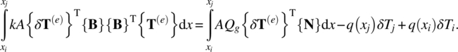
We have substituted Fourier’s law ![]() in the boundary terms in the above equation. Note that the last term on the RHS becomes
in the boundary terms in the above equation. Note that the last term on the RHS becomes ![]() because Ni(xi) = 1 and Ni(xj) = 0. On the other hand, for node j,
because Ni(xi) = 1 and Ni(xj) = 0. On the other hand, for node j, ![]() because the heat flow is positive when the heat enters the element (see figure 4.4). The nodal values are not functions of x and therefore can be taken out of the integrals to rewrite eq. (4.21) as:
because the heat flow is positive when the heat enters the element (see figure 4.4). The nodal values are not functions of x and therefore can be taken out of the integrals to rewrite eq. (4.21) as:
where


In eq. (4.23), we get an expression for the conductance matrix after performing the integration. Similarly, on the RHS, we get the load vector components or the equivalent heat input at node i due to the heat generation term Qg as:

which is the thermal load at node i corresponding to the distributed heat source, and ![]() is the heat flow across the cross section at node i into element e. In eq. (4.22), the nodal values of the virtual temperatures appeared on both sides of the equation and can be canceled out because the virtual temperature is arbitrary and this equation should be valid regardless of the nodal values of the virtual temperature. Therefore, using the principle of virtual work, we obtain the same equation as in the direct method:
is the heat flow across the cross section at node i into element e. In eq. (4.22), the nodal values of the virtual temperatures appeared on both sides of the equation and can be canceled out because the virtual temperature is arbitrary and this equation should be valid regardless of the nodal values of the virtual temperature. Therefore, using the principle of virtual work, we obtain the same equation as in the direct method:

or

where ![]() is the conductance matrix of element e, {Q(e)} is the vector of thermal loads corresponding to the heat source, and {q(e)} is the vector of nodal heat flows across the cross section.
is the conductance matrix of element e, {Q(e)} is the vector of thermal loads corresponding to the heat source, and {q(e)} is the vector of nodal heat flows across the cross section.
When a uniform heat source exists in the element, eqs. (4.24) yield

Note that AQgL(e) is the total heat generated in the element, and it is equally divided between the two nodes.
As mentioned before, the temperature is linear within an element. If the differential equation (4.18) is directly integrated with uniform heat source, the temperature will be a quadratic polynomial. Thus, the finite element solution is approximate, but the error can be reduced by using more elements.
4.5 CONVECTION BOUNDARY CONDITIONS
When a structure is surrounded by a fluid that has a different temperature from the structure, heat flow between the structure and fluid occurs and is called convection. Convection presents a special type of boundary condition called the mixed boundary condition. The closest analogy to this in structural mechanics problems is that of a beam resting on an elastic spring. The convection boundary condition contains an unknown temperature. For example, convective heat flow can be written as
where h is the convection coefficient, S is the area of the exposed surface, and ![]() is the surrounding fluid temperature, which is assumed to be constant. Note that the amount of heat flow is not prescribed. Rather, it is a function of surface temperature, which is unknown.
is the surrounding fluid temperature, which is assumed to be constant. Note that the amount of heat flow is not prescribed. Rather, it is a function of surface temperature, which is unknown.
We will consider two different types of convection heat transfer. In the first case, the convection occurs at the end faces of the one‐dimensional body. For example, the inner surface of the heat chamber in example 4.3 can be exposed to a hot fluid, rather than prescribing a known temperature. The same applies to the outer surface of the ceramic foam in the thermal protection system in example 4.4. In this case, the exposed area S is the same as the cross‐sectional area A. In the second case, the convection heat transfer occurs throughout the length of the one‐dimensional body. For example, an electric wire immersed in water can transfer heat to the surrounding water. This type of convection is not a boundary condition in a strict sense. Rather it is treated as a distributed heat flow. Thus, it should be included in the governing differential equation as in eq. (4.6). In this case, the exposed area S is the perimeter times the length or the exposed area.
4.5.1 Convection on the Boundary
For illustration purpose, consider two one‐dimensional heat transfer elements, as shown in figure 4.14. For simplicity, let us assume that both elements are identical in terms of geometry and material properties. Both ends of the system are under convective boundary conditions. An insulating wall can be an example for this type of problem.

Figure 4.14 Finite element approximation of the furnace wall
Since both elements are identical, the element conduction equations can be written as
element 1:

element 2:

The balance of heat flow in eq. (4.12) can be applied to all nodes in conjunction with convective heat flow in eq. (4.28) as
node 1:
node 2:
node 3:
At nodes 1 and 3, the amount of heat entering the element is equal to the heat transferred by convection, while at node 2 the sum of heat entering elements 1 and 2 is equal to zero.
After substituting the element conduction equation in the balance of heat flow equations, we can assemble the global heat conduction equation as
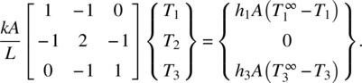
The above equation cannot be solved as it is because the RHS includes unknown nodal temperatures, T1 and T3. This is due to the convection boundary conditions at nodes 1 and 3. In order to solve the above equations, we move the terms containing unknown nodal temperatures to the LHS. Then we obtain the following global equations:

The square matrix in the LHS is nonsingular due to the addition of terms to the diagonal, which makes the matrix positive definite.
4.5.2 Convection along the Length of a Rod
When a long rod is submerged into a fluid, convection occurs across the entire surface. This is different from the previous convection boundary condition in which convection occurs only at the end faces. As shown in figure 4.17, the heat flow in convection is proportional to the perimeter of the cross section multiplied by the length of the rod. In such a case, it is convenient to think of the convection heat flow as a distributed thermal load.

Figure 4.17 Heat conduction and convection in a long rod
The governing differential equation is (see eq. (4.6))

where P is the perimeter of the cross section, that is, P = 2(b + h). The weak form is obtained by multiplying the governing differential equation (4.30) with the virtual temperature δT(x) and integrating over the element length. After replacing the temperature with the approximate temperature in eq. (4.14), we have

We use integration by parts to obtain

Substituting for ![]() , δT, and their derivatives in the integrals on the LHS of eq. (4.32), and rearranging the terms we obtain
, δT, and their derivatives in the integrals on the LHS of eq. (4.32), and rearranging the terms we obtain

One may note that we have substituted Fourier’s law ![]() in the boundary terms in the above equation. Taking the constant nodal values outside the integral and performing the integration, the above equation takes the form
in the boundary terms in the above equation. Taking the constant nodal values outside the integral and performing the integration, the above equation takes the form
where

The thermal load at node i due to the heat generation term Qg and the convection term is given by

and ![]() is the heat flow across the cross section at node i into element e. The nodal values of the virtual temperature, which is a factor on both sides of eq. (4.34), can be canceled out because that equation must be valid for any arbitrary value of {δT(e)}. This yields the following set of element equations:
is the heat flow across the cross section at node i into element e. The nodal values of the virtual temperature, which is a factor on both sides of eq. (4.34), can be canceled out because that equation must be valid for any arbitrary value of {δT(e)}. This yields the following set of element equations:

or
Note that the first matrix on the LHS is the conductance matrix in eq. (4.26), and the equivalent conductance matrix due to convective heat transfer across the periphery is given by

Using the balance of heat flow in eq. (4.12), the above equations can be assembled to obtain the global matrix equations as
Procedures for applying boundary conditions are identical to the previous section.
The thermal load vector on the RHS of eq. (4.36) includes the contribution from the heat source and the convection term. When there is a uniformly distributed heat source Qg, the thermal load in eqs. (4.35) can be integrated to obtain

Note that the total amount of the thermal load is equally divided between the two nodes.
4.6 TWO‐DIMENSIONAL HEAT TRANSFER
A heat conduction problem can be considered two‐dimensional if temperature is constant in one direction, the thickness direction, and all the heat flow occurs in a plane normal to the thickness direction. We will consider the plane where the heat flow occurs as the x‐y plane as shown in figure 4.20 and assume that the temperature is constant in the z‐direction (therefore there is no heat flow in that direction).

Figure 4.20 Two‐dimensional heat transfer analysis domain
The three types of boundary conditions we described for the one‐dimensional problem are also applicable to two‐dimensional heat transfer problems. In some parts of the boundary ST, the temperature may be known and fixed, while at other parts of the boundary, SQ, heat flux may be known or the heat flux may be due to convection, Sh. The geometry is assumed to be of constant thickness t in the z‐direction; therefore, we can consider a two‐dimensional area as shown in the figure to be the domain of analysis where we need to compute temperature as a function of (x,y) coordinates. In this section, we will develop necessary equations for energy equilibrium using the Galerkin's method. In the following section, we would like to divide this domain into elements and describe the temperature field using nodal values while interpolating within each element to approximate the solution.
4.6.1 Boundary Value Problem for Two‐Dimensional Heat Transfer
Equilibrium equation for heat balance:
Similar to the one‐dimensional heat transfer problem, the governing equations of two‐dimensional heat transfer are the equilibrium equations, which can be easily derived from the energy balance condition. Consider a two‐dimensional infinitesimal element shown in figure 4.21 that is in equilibrium. The heat flow into the element is equal to the heat flowing out of the element.

Figure 4.21 Energy balance in an infinitesimal element
In two dimensions, the heat flux density is a vector that represents the rate of heat flow per unit area, and it is denoted here as ![]() . The energy balance is stated below as the sum of heat flowing in and out of the system in the x and y direction and the heat generated Qg within the system should add up to zero:
. The energy balance is stated below as the sum of heat flowing in and out of the system in the x and y direction and the heat generated Qg within the system should add up to zero:
As the heat flux density is per unit area, we multiply each term with the area across which the heat is flowing; that is, tdy for the surface normal to x‐axis and tdx for the surface normal to y‐axis. The thickness t can be canceled out from this equation as it occurs as a factor in all the terms, or equivalently, we can assume the equation is for unit thickness. Then, the area of the faces normal to the x‐ and y‐directions are dy and dx, respectively, and the volume of the differential element is dxdy. The terms in parentheses represent the net rate of heat flux in the x‐ and y‐directions. Expanding them using the first‐order Taylor series expansion, we get

Substituting, these into the energy balance equation (4.40), we get the following partial differential equation as the equilibrium equation:

Or, after canceling the volume term, we have
In would be informative if the above equation is compared with the governing equation for the one‐dimensional problem in eq. (4.5). In the limit as the size of the differential element shrinks to zero, this equilibrium condition must apply at every point within the domain of analysis. Note that this equation does not yet involve temperature, which is the quantity we are interested in solving for. We need a relation between the heat flux and the temperature in order to rewrite this equation with temperature as the variable. This relation depends on the material through which heat transfer is occurring and is referred to as the constitutive equation. We need to develop a similar relationship given in eq. (4.1) for the case of the two‐dimensional problem.
Constitutive equation (Fourier’s law):
The constitutive equation for heat conduction is Fourier’s law, which states that heat flux is proportional to the negative of temperature gradient. In other words, heat flows in the direction of decreasing temperature at a rate that is proportional to the rate at which temperature is decreasing. The proportionality constant is a material property, which is referred to as the thermal conductivity of the material. In the most general form, such a constitutive equation can be stated as:

In the preceding equations, the heat flux densities in the x‐ and y‐directions are written as proportional to the components of the temperature gradient. This equation can be restated as a matrix equation, where the material constants are all collected into a conductivity matrix, as

where ![]() is called the gradient operator. When a function is multiplied with the gradient operator, it becomes the gradient vector of the function; for example,
is called the gradient operator. When a function is multiplied with the gradient operator, it becomes the gradient vector of the function; for example, ![]() is the column vector of temperature gradient.
is the column vector of temperature gradient.
In practice, for most materials, the heat flux in any direction depends only on the component of temperature gradient in that direction1. In other words, heat conduction in the x‐direction does not occur due to a temperature gradient in the y‐direction. Therefore, the off‐diagonal terms in the conductivity matrix are usually zero; that is, ![]() . Furthermore, if the material is isotropic, then the conductivity is the same in all directions. Therefore, for all isotropic materials
. Furthermore, if the material is isotropic, then the conductivity is the same in all directions. Therefore, for all isotropic materials ![]() , and we can simplify Fourier’s law to
, and we can simplify Fourier’s law to

Governing differential equations:
The governing equation can be obtained by substituting the constitutive equation into the equilibrium equation (4.44). For two‐dimensional heat conduction, the governing equation that must be satisfied at every point in the domain for equilibrium is

This equation can be generalized to the three‐dimensional problem by including the components in the z‐direction as well. Using the notation of vector calculus, the governing equation can be stated more succinctly as
In the case of isotropic materials, the above equations can be further simplified as
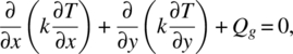
and
These governing equations cannot be solved on their own to determine the temperature field. To fully define the problem, one needs to also define the domain of analysis and the boundary conditions that apply along its boundaries.
Boundary Value Problem: The domain of analysis for two‐dimensional problems is an area as shown in figure 4.20. The boundary of this region can divided into different regions based on the type of boundary conditions that are applied. In the figure, regions subjected to temperature boundary conditions are labeled as ST. Similarly, the parts of boundary subjected to heat flux boundary conditions and convection are named SQ and Sh, respectively. It is assumed that these boundaries compose the entire boundary and do not overlap; that is, mathematically, ![]() and
and ![]() . Even though each of these regions on the boundary is shown as connected, it is not always be the case. For instance, it is possible that the heat flux is specified at two different parts of the boundary that are not adjacent to each other. In this case, SQ is not a connected region but a union of all the regions where heat flux is specified on the boundary. Similarly, ST and Sh could also be disconnected regions on the boundary. It should also be noted that if no boundary condition is specified in a particular region of the boundary, that region would be part of SQ because it is implied that there is no heat flux on the boundary or, in other words, the heat flux at that boundary is known to be zero.
. Even though each of these regions on the boundary is shown as connected, it is not always be the case. For instance, it is possible that the heat flux is specified at two different parts of the boundary that are not adjacent to each other. In this case, SQ is not a connected region but a union of all the regions where heat flux is specified on the boundary. Similarly, ST and Sh could also be disconnected regions on the boundary. It should also be noted that if no boundary condition is specified in a particular region of the boundary, that region would be part of SQ because it is implied that there is no heat flux on the boundary or, in other words, the heat flux at that boundary is known to be zero.
In two‐dimensional heat transfer problems, the goal is to solve for the temperature field T(x, y) in the given area of material, A, while satisfying all the specified boundary conditions. The boundary value problem to be solved for this purpose may be stated as follows:
Solve T(x, y) in A such that

where ![]() is the normal component of the heat flux on the boundary, and
is the normal component of the heat flux on the boundary, and ![]() is the temperature of the surrounding fluid. The negative sign in q0 is because qn is the heat flux out to the system, while by definition, q0 is the heat flux coming into the system.
is the temperature of the surrounding fluid. The negative sign in q0 is because qn is the heat flux out to the system, while by definition, q0 is the heat flux coming into the system.
To keep our notations simple, we have assumed that the material is isotropic and used the scalar k for conductivity. We will use that assumption for the rest of the chapter with understanding that it can be replaced with the conductivity matrix if the material is anisotropic.
4.6.2 Galerkin’s Method for Two‐Dimensional Heat Conduction
The boundary value problem in eq. (4.52) states that the governing equation, which is a partial differential equation, must be satisfied at every point in the domain of interest while simultaneously satisfying all the boundary conditions. As we discussed in chapter 2, the solution to the boundary value problem is called the exact solution. In finite element analysis, we are looking for an approximate solution that satisfies the essential boundary conditions but not necessarily the natural boundary conditions. In this section, we use Galerkin’s method in section 2.4 of chapter 2 to derive the governing equation that will be used for finite element analysis. In this approach, we first multiply the governing equation by a virtual temperature and integrate over the area, as

If the governing equation is satisfied at every point in the area A, then the above equation will be satisfied regardless of the nature of the virtual temperature δT, which is an arbitrary scalar field defined over the area A. Equation (4.53) is an approximation in the sense that it could be satisfied even if the governing equation is not strictly satisfied at every point and the residual is nonzero at some locations. Such error or residual is tolerated because the errors in different parts can cancel each other out, and the equation is satisfied in an average sense. This tolerance of error or nonzero residual is an important property that allows us to compute approximate solutions, and therefore we refer to this equation as a weak form. Then we use integration by parts to derive a more convenient form, as we did for one‐dimensional problems in chapter 2. The equivalent of integration by parts for a two‐dimensional problem is the Green’s theorem. For convenience, we provide Green’s theorem below:
Expanding eq. (4.53) using Green’s theorem, we get a more convenient weak form that involves only the first derivatives of the temperature and the virtual temperature. Using this theorem, on the first part of eq. (4.53) we obtain

Substituting this into eq. (4.53), we obtain the following integral equation that is the starting point for formulating the discretized finite element equations:

The boundary integral over S can be split into three parts:

Here we have used the relationship ![]() . Along ST, since the temperature is known, the virtual temperature vanishes, that is,
. Along ST, since the temperature is known, the virtual temperature vanishes, that is, ![]() . Therefore, there is no contribution to the RHS from this part of the boundary. It is also important to note that the normal component of heat flux at this boundary is unknown. Indeed, to keep the temperature constant at this boundary, some heat has to flow through this boundary but it is an unknown quantity similar to the reaction at a fixed boundary for structural problems.
. Therefore, there is no contribution to the RHS from this part of the boundary. It is also important to note that the normal component of heat flux at this boundary is unknown. Indeed, to keep the temperature constant at this boundary, some heat has to flow through this boundary but it is an unknown quantity similar to the reaction at a fixed boundary for structural problems.
Along the SQ boundary, since the heat flux is known, we can write the contribution to the RHS due to this part of the boundary as

Note that ![]() is the normal component of the heat flux flowing out of the area A because the unit normal n points to the outside of the analysis domain A. Therefore, if q0 is the known heat flux coming into the system, then
is the normal component of the heat flux flowing out of the area A because the unit normal n points to the outside of the analysis domain A. Therefore, if q0 is the known heat flux coming into the system, then ![]() .
.
For convection boundary, the normal component of the heat flux flowing out of the volume is proportional to the difference between the surface temperature and the surrounding air temperature or the ambient temperature ![]() :
:
The proportionality constant, h, is the convection coefficient. Using this relation, we can write the contribution from the convection boundary as

Substituting the contribution from surface integrals along ST, SQ, and Sh, we can rewrite the weak form in eq. (4.55) in the final form as follows:

It is apparent in the above equation that all the information from the original boundary value problem is incorporated, except for the temperature boundary condition on ST. Therefore, the approximate temperature of finite element analysis should satisfy the temperature boundary condition, while other boundary conditions will be satisfied as a part of the analysis. The terms that involve the unknown temperature have been moved to the left‐hand side while known quantities are on the right. As a result, the convection has a contribution to both sides of this equation.
Galerkin’s method yields an integral equation where the integration must be carried out over any arbitrary structural geometry. To facilitate this integration, it is convenient to break up the geometry into simpler shapes called finite elements. The most commonly used elements for two dimensions are triangles and quadrilaterals. The process of subdividing the geometry into elements is called mesh generation wherein elements are created, and nodes are placed at the vertices, edges, or midpoints of these elements. The discretized geometry consisting of nodes and elements is referred to as the mesh. These nodes are shared between adjacent elements if two or more elements meet at a node. The mesh then serves as an approximation of the structural geometry. It is also used for approximating the solution by interpolating the nodal values within each element. In Galerkin’s approach, we assume that the virtual temperature δT is interpolated within each element using the same shape functions as the temperature field. In this chapter, we will use a 3‐node triangular element to illustrate the process of deriving the interpolation scheme as well as discretizing the weak form into a set of linear simultaneous equations. Elements that use higher‐order interpolation will be introduced in chapters 6 and 7.
4.7 3‐NODE TRIANGULAR ELEMENTS FOR TWO‐DIMENSIONAL HEAT TRANSFER
The simplest way of dividing a planar region into elements is to use triangular elements. Figure 4.22 shows a planar region that is divided into triangular elements. Each element shares its edges and nodes with adjacent elements if any. The three vertices of a triangle are the nodes of that element as shown in figure 4.22. The first node of an element can be arbitrarily chosen. However, the sequence of the nodes 1, 2, and 3 should be in the counterclockwise direction.

Figure 4.22 3‐node triangular element
The temperature within the element is interpolated using the nodal values of temperature using interpolation functions, better known as shape functions. The temperature field within the element is assumed to be a polynomial function whose coefficient must be determined by using the nodal values. For this element, the temperature field has to be a linear function in x and y because values of temperature are available only at three points (nodes), and a linear polynomial has three unknown coefficients. As the temperature is a linear function, its gradient is a constant within an element, and therefore, the heat flux density is a constant vector for each element in a mesh consisting of 3‐node triangular elements. The heat flux density is of course not likely to be constant in the exact solution, and therefore, this element provides an approximate solution and should be used with caution. The elements in the mesh should be very small so that the piecewise constant heat flux density can reasonably approximate the real heat flux density field. Later we will see higher‐order elements that provide better approximation.
4.7.1 Temperature Interpolation
The first step in deriving the finite element matrix equation is to interpolate the temperature function in terms of the nodal temperatures. Clearly, the interpolated function must be a linear, three‐term polynomial in x and y of the form:
where, the α’s are constants to be determined. In finite element analysis, we would like to replace these constants by determining their value in terms of the nodal temperatures. At node 1, for example, x and y take the values of x1 and y1, respectively, and the nodal temperature is T1. If we repeat this for the other two nodes, we obtain the following three simultaneous equations:

In matrix notation, the above equations can be written as
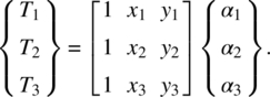
If the three points, (x1, y1), (x2, y2), and (x3, y3), are not on a straight line, then the inverse of the above coefficient matrix exists. Thus, we can calculate the unknown coefficients as

where Ae is the area of the triangle and
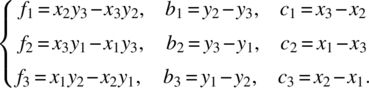
The area Ae of the triangle can be calculated from

Note that the determinant in eq. (4.67) is zero when three nodes are collinear. In such a case, the area of the triangular element is zero, and we cannot uniquely determine the three coefficients. After calculating αi the temperature interpolation can be written as

where the shape functions are defined by

or
Note that N1(x,y), N2(x,y), and N3(x,y) are linear functions of x‐ and y‐coordinates. Thus, interpolated temperature varies linearly in each coordinate direction.
After calculating the temperature field within an element, the gradient of temperature can be calculated by differentiating the temperature with respect to x and y. For example, the derivative with respect x can be written as

Note that T1, T2, and T3 are nodal temperatures, and they are independent of the x‐coordinate. Thus, only the shape function is differentiated with respect to x. Using the matrix notation, the temperature gradient can be written as

It may be noted that the [B]T matrix is constant and depends only on the coordinates of the three nodes of the triangular element. Thus, one can anticipate that if this element is used, then the temperature gradient will be constant over a given element and will depend only on nodal temperatures.
4.7.2 Conductance Matrix for 3‐Node Triangular Element
The weak form in the previous section involves area integrals over the entire domain of analysis. This integral can now be split into integrals over individual elements in the mesh. The conductance term on the left‐hand side (LHS) of eq. (4.61) can be written as the sum of the integration over all the elements in the mesh, as

where NEL is the total number of elements in the system. The temperature field and its gradient were expressed in the matrix form using the shape functions of the three‐node triangular element in the last section. These can now be used to write discretized equations for each element. In Galerkin’s approach, we assume that the virtual temperature is also interpolated using the same shape functions as the temperature. Therefore, we can write these as,

Substituting, these matrix expressions for temperature and the weighting function, we can rewrite the conductance term on the LHS of eq. (4.61) in the following matrix form:

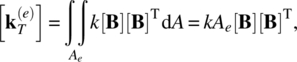
where ![]() is the element conductance matrix for heat transfer and is analogous to the stiffness matrix computed for structural mechanics problems. Note that all the matrices within the integral are constant matrices for this element. Therefore, the conductance matrix can be computed as
is the element conductance matrix for heat transfer and is analogous to the stiffness matrix computed for structural mechanics problems. Note that all the matrices within the integral are constant matrices for this element. Therefore, the conductance matrix can be computed as

4.7.3 Thermal Loads for a 3‐Node Triangular Element
Thermal load due to distributed heat source:
The right‐hand side (RHS) of eq. (4.61) contains an area integral, which corresponds to the thermal load due to the distributed heat source. An example of the distributed heat source is when there is heat being generated in the entire area of a solid due to electrical current flow. This term can also be discretized in a similar fashion to express it in a matrix form. The contribution of the distributed heat source or heat generation term for an element e can be expressed as:

where

is the thermal load due to the distributed heat source.
In later chapters, we will discuss numerical methods for integrating over triangles. For the 3‐node triangles, the integration of the shape functions over the area of the triangle is rather straightforward as it is equivalent to finding the volume under the function Ni(x, y). Figure 4.23 shows the plot of a typical linear shape function over a triangular element. At node 1, the value of the shape function ![]() . The volume under the shape function is the tetrahedron whose height is one and its base is the area of the triangle, therefore,
. The volume under the shape function is the tetrahedron whose height is one and its base is the area of the triangle, therefore,
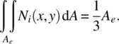
Here, we use the well‐known result that the volume of the tetrahedron is one‐third of the product of its height and the area of the base.
Figure 4.23 Plot of linear shape function for triangular element
Assuming the heat source is uniformly distributed within the element, the thermal load due to the distributed heat source can be calculated as

Load due to applied heat flux:
The integral over SQ on the right‐hand side of eq. (4.61) is the contribution due to known heat flux entering the domain. This term contributes only to the thermal load vector of the elements that are on the boundary SQ. To evaluate this term, we need to integrate along the edges of the elements that are on this boundary.


Here we have assumed that the virtual temperature δT is interpolated in the same fashion as the temperature. As δT is linearly interpolated over the element, we expect that δT is interpolated along the edge using linear shape functions. To interpolate nodal values of the edge nodes, we construct linear shape functions ![]() and use them to interpolate δT along the edge as:
and use them to interpolate δT along the edge as:
where the shape functions on the edge {N′} and nodal temperature on the edge {δT(e)′} are defined as ![]() and
and ![]() , respectively.
, respectively.
The shape function vector {N′} consists of the linear shape functions that interpolate δT along the edge of the element and {δT(e)′} containing the nodal values of δT. Figure 4.24 shows an element where a heat flux is applied to the edge between nodes 1 and 2. The local coordinate s has origin at node 1 and measures the distance from this node. The linear shape functions ![]() and
and ![]() are plotted along these edges. If we assume that the heat flux is constant along the edge, then we have
are plotted along these edges. If we assume that the heat flux is constant along the edge, then we have

The linear shape functions derived earlier for one‐dimensional elements in eq. (4.15) can be used here too after writing them in terms of the local coordinate system s shown in figure 4.24.

Figure 4.24 Linear shape functions for interpolation along edge

where Le is the length of the edge 1‐2 of the element. To evaluate the load due to heat flux, these shape functions can be integrated over s from 0 to Le. We can evaluate the integral by making use of the fact that the area under the shape functions ![]() and
and ![]() is equal to half the length of the edge of the triangle Le.
is equal to half the length of the edge of the triangle Le.

Convection boundary condition:
The contribution of the convection heat transfer is the integral over Sh, which was split into two parts in eq. (4.61). Again, we need to integrate along the edges of the elements that are on this boundary to evaluate this boundary integral, and as before we will interpolate δT linearly using the shape functions in (4.83). Consider the convection term on the LHS of eq. (4.61) first, as

where
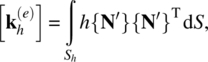


Along the edge of the element, both δT and T are interpolated linearly, and {δT(e)′} is again a 2 × 1 column vector that contains that nodal values of δT for that edge. The effective conductance matrix ![]() due to convection is a 2 × 2 matrix for elements on a convection boundary. This matrix is to be assembled into the global conductance matrix along with the conductance matrix of all the other elements.
due to convection is a 2 × 2 matrix for elements on a convection boundary. This matrix is to be assembled into the global conductance matrix along with the conductance matrix of all the other elements.
On the right‐hand side of eq. (4.61), the contribution due to convection is similar to a heat flux vector:


So far, we have looked at how the contribution from each element in the mesh is computed in the form of element stiffness matrices and thermal load vectors. These contributions must be assembled into a global system of equations. This process can be best understood by looking at a simple example that shows the entire process. The essential boundary conditions are imposed after assembling the global equations.
4.8 FINITE ELEMENT MODELING PRACTICE FOR 2‐D HEAT TRANSFER
The finite element method is most useful when applied to two‐ and three‐dimensional problems with complex geometries for which no analytical solutions are available. For such problems, a large number of nodes and elements are typically needed, which makes it necessary to use software for the analysis. In this section, we look at some practical aspects to consider when constructing finite element models. These aspects include deciding types of boundary conditions and thermal load conditions that can represent the real physical system, as well as understanding periodicity and symmetry to simplify the physical model.
4.8.1 Heat Conduction in a Slab
A series of pipes carrying hot fluids are embedded in a slab. The spacing between pipes is 40 mm and the thickness of the slab is ![]() mm. The surfaces of the block are exposed to air with ambient temperature of 30oC. The heat transfer takes place due to conduction between the pipes and the block and due to convection to the ambient air. The conductivity of the slab is
mm. The surfaces of the block are exposed to air with ambient temperature of 30oC. The heat transfer takes place due to conduction between the pipes and the block and due to convection to the ambient air. The conductivity of the slab is ![]() W/mmoC and the convection coefficient is assumed to be
W/mmoC and the convection coefficient is assumed to be ![]() W/mm2oC. We wish to determine the temperature distribution in the block.
W/mm2oC. We wish to determine the temperature distribution in the block.
Assuming that the slab extends much further in either direction and that the spacing between pipes is constant through the slab, we have a repeating pattern creating a periodic structure. We can make use of this periodicity to identify a rectangular region of the slab that contains just one single pipe as shown by the shaded region in figure 4.27(a). This is a unit cell, which repeats periodically in both directions. We need to model only one such unit cell, instead of modeling the entire slab, because we expect to find the same temperature distribution within any such cell within the slab. The unit cell is symmetric both vertically and horizontally. Therefore, making use of the symmetry, we can further simplify the model to a quadrant of the unit cell as shown in figure 4.27(b). For this two‐dimensional model, we assume the depth of the model in the z‐direction to be unity or in other words, we are modeling a unit depth of the slab. A temperature boundary condition (T = 100 °C) is applied to the circular edge, which represents the outside surface of the embedded pipe. One could argue that if the pipes contain hot fluid, then it may be more appropriate to use a convection boundary condition for the pipe surface. However, if the convection coefficient is sufficiently large, for example due to the high velocity of the fluid flow, then the temperature at the surface will be very close to the fluid temperature, and therefore a boundary condition specifying temperature at the boundary to be equal to the fluid temperature is justified. The correct boundary condition for any model depends on the real system being modeled. Therefore, it is very important to have a very good understanding of the system and the applicable material properties and parameters to arrive at the best model. Convection boundary condition is applied on the outer surface of the slab.

Figure 4.27 Finite element model for slab with pipes: (a) periodicity and symmetry, (b) model
On the remaining edges, no boundary conditions or thermal loads are applied. This is equivalent to a zero heat flux condition on these boundaries, as if these boundaries were insulated. It is important to understand why such a boundary condition is appropriate. The reason has to do with the fact that these boundaries are symmetry boundaries, and therefore two neighboring points equidistant from these boundaries on its two sides will have the same temperature. This implies that the gradient of temperature normal to the boundary will be zero, and therefore the heat flux across the boundary will also be zero.
Figure 4.28 shows the temperature distribution in the slab computed using the finite element model described above. Figure 4.28(a) shows a continuous distribution plot while (b) shows discrete or fringe plots of the temperature. These are the two most common ways in which finite element analysis software programs display the solution. Some software programs are also able to plot contours of the variable. The contours of the temperature plot are also seen in the fringe plot. The contours provide useful visual information because the gradient of temperature and the heat flux are normal to these contours. It can be seen that the contours are horizontal near the vertical edges, which indicates that the heat flux is parallel to these vertical edges, and therefore the heat flux normal to these edges are zero as expected. Similarly, the heat flux component in the vertical direction is zero at the horizontal symmetric line.

Figure 4.28 Temperature distribution in the slab
The horizontal and vertical heat flux components are plotted in figure 4.29. Again, it can be seen that the horizontal component is nearly zero near the vertical edges of symmetry while the vertical component is zero at the horizontal symmetric edge.

Figure 4.29 Heat flux components in the slab
The exact solution for the temperature distribution, its gradient, and the heat flux are all expected to be continuous functions. The heat flux shown in the figures suggests that this was true for the computed solution as well. However, we stated earlier that the triangular element computes a piecewise linear solution, and therefore, the heat flux will be constant within each element. In this case, the color within each element should be constant, and the heat flux distribution should be discontinuous. This raises the question about why the color plot of the heat flux appears continuous. This is because in most finite element analysis software, the heat flux (and also stresses and strains) are smoothed before plotting. There are many ways to perform the smoothing operation. A simple algorithm would compute the average value at the nodes by averaging the heat flux computed for each element that connects to that node. Then these averaged values are interpolated within each element to determine the heat flux values inside the triangular element.
Approximating the heat flux as constant within each element is not very desirable or accurate, and in fact, the smoothed results are closer to the real solution. The 3‐node triangular element is not a very good element due to the piecewise linear approximation that it provides. A very dense mesh, that is, a mesh with very large number of small elements is needed to get even a reasonable or acceptable answer. Better elements can be derived if we assume that the temperature distribution is quadratic or even higher‐order within each element. In later chapters, we will see other types of elements including higher‐order triangular and quadrilateral elements that can be used to solve the heat conduction and solid mechanics problems.
4.9 EXERCISES
- Answer the following descriptive questions.
- In finite elements for solid mechanics, nodal forces are defined as positive when the force is applied in the positive coordinate direction. How is the positive heat flux defined for an element?
- Two 1‐D heat transfer elements have the same thermal conductivity and cross‐sectional area but have different lengths. When the temperature differences between the two nodes of the two elements are the same, which element has a higher heat flow? A long element or a short one?
- In solid mechanics, when a node is fixed, the column corresponding to the fixed DOF is deleted (strike the column). In heat transfer analysis, how can a prescribed temperature be imposed in the global matrix equation?
- In the weak form of Galerkin’s method, when the temperature at node i, Ti, is prescribed, what is the value of the weighting function δTi at that node?
- The wall of a heat chamber is modeled with three 1‐D elements, where each element has different length. There is no heat generation within the wall. Will the heat flux for the three elements be the same or different? Explain why.
- Explain how a convection boundary condition makes the finite element matrix positive definite without striking the row or striking the column.
- Consider heat conduction in a uniaxial rod surrounded by a fluid. The left end of the rod is at T0. The free stream temperature is
 . There is convective heat transfer across the surface of the rod as well over the right end. The governing equation and boundary conditions are as follows:where k is the thermal conductivity, h is the convective heat transfer coefficient, and A and P are the area and circumference of the rod’s cross section, respectively. The numerical values (SI units) are: L = 0.5, k = 200, h = 10, T0 = 700,
 = 400, A = 10−4, P = 4 × 10⁻². Use three finite elements to solve the problem. Use elements of lengths 0.1, 0.15, and 0.25, respectively.
 - Consider the heat conduction problem shown in the figure. Inside the bar, heat is generated from a uniform heat source Qg = 10 W/m3, and the thermal conductivity of the material is k = 0.2 W/m/°C. The cross‐sectional area A = 1 m2. When the temperatures at both ends are fixed to 0 °C, calculate the temperature distribution using: (a) two equal‐length elements and (b) three equal‐length elements. Plot the temperature distribution along the bar and compare with the exact solution.

- Repeat problem 3 with Qg = 20x.
- Determine the temperature distribution (nodal temperatures) of the bar shown in the figure using two equal‐length finite elements with cross‐sectional area of 1 m2. The thermal conductivity is 15 W/m⋅°C. The left side is maintained at 300 °C. The right side is subjected to heat loss by convection with h = 1.5 W/m2⋅°C and Tf = 30 °C. All other sides are insulated.

- The nodal temperatures of a 1‐D heat conduction problem are given in the figure. Calculate the temperature at x = 0.2 using: (a) two 2‐node elements and (b) one 3‐node element.

- In order to solve a 1‐D steady‐state heat transfer problem, one element with 3‐nodes is used. The shape functions and the conductivity matrix before applying boundary conditions are given.

- When the temperature at node 1 is equal to 50 °C and a heat flux of 80 W is provided at node 3, calculate the temperature at x = ¼ m.
- When the temperature at node 1 is equal to 50 °C and the convection boundary condition is applied at node 3 with h = 4 W/m2/°C, T∞ = 120 °C, calculate the temperature at x = ¼ m.
- Instead of the previous boundary conditions, heat fluxes at nodes 1 and 3 are given as Q1 and Q3, respectively. Can this problem be solved for the nodal temperatures? Explain your answer.

- The one‐dimensional wall in the figure is modeled using one element with three nodes. There is a uniform heat source inside the wall generating Q = 200 W/m3. The thermal conductivity of the wall is k = 2 W/(m⋅°C). Assume that A = 1 m2 and l = 1 m. The left end has a fixed temperature of T = 20 °C, while the right end has zero heat flux.
- Calculate the shape function [N] = [N1, N2, N3] as a function of x.
- Solve for the nodal temperature {T} = {T1, T2, T3}T using boundary conditions. Plot the temperature distribution in an x‐T graph.
- Calculate the heat fluxes at x = 0 and x = 1 when the solution is {T} = {20, 58.25, 71}.

- Consider heat conduction in a uniaxial rod surrounded by a fluid. The right end of the rod is attached to a wall and is at temperature TR. One half of the bar is insulated as indicated. The free stream temperature is Tf. There is convective heat transfer across the un‐insulated surface of the rod as well as over the left‐end face. Use two equal‐length elements to determine the temperature distribution in the rod. Use the following numerical values: L = 0.2 m, k = 100 W/m/°C, h = 26 W/m2/°C, TR = 600 °C, Tf = 300 °C, A = 10−4 m2, and P = 0.04 m.

- A well‐mixed fluid is heated by a long iron plate of conductivity k = 10 W/m/°C and thickness t = 0.12 m. Heat is generated uniformly in the plate at the rate Qg = 5,000 W/m3. If the surface convection coefficient h = 5 W/m2/°C and fluid temperature is Tf = 45 °C, determine the temperature at the center of the plate, Tc, and the heat flow rate to the fluid, q, using three one‐dimensional elements.

- A cooling spine of square cross‐sectional area A = 0.25 × 0.25 m2, length L = 2 m, and conductivity k = 10 W/m/°C extends from a wall maintained at temperature Tw = 200 °C. The surface convection coefficient between the spine and the surrounding air is h = 0.6 W/m2/°C, and the air temperature is Ta = 20 °C. Determine the heat conducted by the spine and the temperature of the tip using five one‐dimensional finite elements.

- Find the heat transfer per unit area through the composite wall in the figure. Assume one‐dimensional heat flow and that there is no heat flow between B and C. The thermal conductivities are kA = 0.04 W/m/°C, kB = 0.2 W/m/°C kC = 0.03 W/m/°C, and kD = 0.06 W/m/°C.

- Consider a wall built up of concrete and thermal insulation. The outdoor temperature is To = −20 °C, and the temperature inside is Ti = 20 °C. The wall is subdivided into three elements. The thermal conductivity for concrete is kc = 2 W/m/°C, and that of the insulator is ki = 0.05 W/m/°C. Convection heat transfer is occurring at both surfaces with convection coefficients of h0 = 14 W/m2/°C and hi = 5.5 W/m2/°C. Calculate the temperature distribution of the wall. Also, calculate the amount of heat flow through the outdoor surface.

- The heat conduction through the thickness of a plate can be modeled as a single 1‐D quadratic (3‐node) element assuming that the plate is large with uniform temperature on the same thickness. The temperature at x1 is fixed at 100 °C while x2 is at 25 °C. Heat is being generated within the plate at the rate of Qg =1000 W/m3. The conductivity of the plate is
 W/(mm°C), and the thickness of the plate is 10 mm. When the shape functions and conductivity matrix are given,
- compute the nodal equivalent heat source corresponding to the heat generation in the plate.
Hint: ; and
; and - determine the temperature distribution T(r). Note k is conductivity, A = area, L(e) = length of the element.

- compute the nodal equivalent heat source corresponding to the heat generation in the plate.
- The shape functions of a linear 3‐node element are also called barycentric or area coordinates because they uniquely define the location of a point in the triangle. Show that the shape functions in eq. (4.69) can also be computed as:where A1 is the area of triangle P23 in the figure, A2 is the area of triangle P13, A3 is the area of triangle P12, and

 is the area of triangle 123.