
Chapter 5
Review of Solid Mechanics
5.1 INTRODUCTION
The finite element method is a powerful numerical method for solving partial differential equations. It has been applied to solve many physical problems whose governing equations are partial differential equations. The method has been implemented and is available as commercial software that can perform a variety of analysis including solids, structures, and thermal systems to mention a few. However, to use these programs effectively, one must understand the underlying physics of the problem being solved. This is important not only to be able to construct the right models for analysis but also to interpret the results and verify its accuracy. In this chapter, we review the main principles and the governing equations of solid mechanics. We explain the physical meaning behind the stress and strain tensors and the relation between them. Stress analysis is a major step, and in fact, it can be considered the most important one in the mechanical design process. There are many design considerations that influence the design of a machine element or structure. The most important design considerations are the following1: (i) the stress at every point should be below a certain limit for the material; (ii) the deflection should not exceed the maximum allowable for proper functioning of the system; (iii) the structure should be stable; and (iv) the structure or machine element should not fail due to fatigue. The failure mode corresponding to instability is also referred to as buckling. The failure due to excessive stress can take different forms such as brittle fracture, yielding of the material causing inelastic deformations, and fatigue failure. Stress analysis of structures plays a crucial role in predicting failure types (i), (ii), and (iv) above. The analysis of stability of a structure requires a slightly different approach but in general, uses most of the methods of stress analysis. Often, the results from the stress analysis can be used to predict buckling. Thus, stress is often used as a criterion for mechanical design.
In the elementary mechanics of materials or physics courses, stress is defined as force per unit area. While such a notion is useful and sufficient to analyze one‐dimensional structures under a uniaxial state of stress, a complete understanding of the state of stress in a three‐dimensional body requires a thorough understanding of the concept of stress at a point. Similarly, the strain is defined as the change in length per original length of a one‐dimensional body. However, the concept of strain at a point in a three‐dimensional body is quite interesting and is required for a complete understanding of the deformation a solid undergoes. While stresses and strains are concepts developed by engineers for a better understanding of the physics of deformation of a solid, the relation between stresses and strains is phenomenological in the sense that it is something observed and described as a simplified theory. Robert Hooke2 was the first to establish the linear relation between stresses and strains in an elastic body. Although he explained his theory for one‐dimensional objects, later his theory became the generalized Hooke’s law that relates the stresses and strains in three‐dimensional elastic bodies.
In this chapter, we will introduce three‐dimensional stresses and strains as second‐order tensor quantities and study some of their properties. We will then present three‐dimensional stress‐strain relationship for isotropic, linear elastic materials and discuss three different types of two‐dimensional solid mechanics problems. The solid mechanics boundary value problem and the principle of minimum potential energy will be presented as the basic equations to be solved to obtain the displacement field. Thereafter, we discuss various failure theories that are used while designing structures against failure.
5.2 STRESS
5.2.1 Surface Traction
Consider a solid subjected to external forces and in static equilibrium as shown in figure 5.1. We are interested in the state of stress at a point P in the interior of the solid. We cut the body into two halves by passing an imaginary plane through P. The unit vector normal to the plane is denoted by n [see figure 5.1(b)]. The portion of the body on the left side is in equilibrium because of the external forces f1, f2, and f3 and also the internal forces acting on the cut surface. “Surface traction” is defined as the internal force per unit area or the force intensity acting on the cut plane. In order to measure the intensity or traction specifically at P, we consider the force ΔF acting over a small area ΔA that contains point P. Then the surface traction T(n) acting at the point P is defined as

Figure 5.1 Surface traction acting on a plane at a point
In eq. (5.1), the right superscript (n) is used to denote the fact that this surface traction is defined on a plane whose normal is n. It should be noted that at the same point P the traction vector T would be different on a different plane passing through P. It is clear from eq. (5.1) that the dimension of the traction vector is the same as that of pressure, or force per unit area.
Since T(n) is a vector, one can resolve it into Cartesian components and write it as
and its magnitude can be computed from
5.2.2 Normal Stresses and Shear Stresses
The surface traction T(n) defined by eq. (5.1) does not act in general in the direction of n, that is, T and n are not necessarily parallel to each other. Thus, we can decompose the surface traction into two components, one parallel to n and the other perpendicular to n, which will lie on the plane. The component normal to the plane or parallel to n is called the normal stress and is denoted by σn. The other component, parallel to the plane or perpendicular to n, is called the shear stress and is denoted by τn.
The normal stress can be obtained from the scalar product of T(n) and n, as (see figure 5.3)
and the shear stress can be calculated from the relation

Figure 5.3 Normal and shear stresses at a point P
The angle between T(n) and n can be obtained from the definition of scalar product given in eq. (A.18) in the appendix.
5.2.3 Rectangular or Cartesian Stress Components
The surface traction at a point varies depending on the direction of the normal to the plane, and therefore, one can obtain an infinite number of traction vectors T(n) and corresponding normal and shear stresses for a given state of stress at a point. However, one might be interested in the maximum values of these stresses and the corresponding plane. Fortunately, the state of stress at a point can be completely characterized by defining the traction vectors on three mutually perpendicular planes passing through the point. That is, from the knowledge of T(n) acting on three orthogonal planes, one can determine T(n) on any arbitrary plane passing through the same point. For convenience, these planes are taken as the three planes that are normal to the x, y, and z axes.
Let us denote the traction vector on the yz–plane, which is normal to the x‐axis, as T(x). Instead of decomposing the traction vector into its normal and shear components, we will use its components parallel to the coordinate directions and denote them as ![]() , and
, and ![]() . That is,
. That is,
It may be noted that ![]() in eq. (5.6) is the normal stress, and
in eq. (5.6) is the normal stress, and ![]() and
and ![]() are the shear stresses in the y‐ and z‐directions, respectively. In contemporary solid mechanics, the stress components in eq. (5.6) are denoted by σxx, τxy, and τxz, where σxx is the normal stress, and τxy and τxz are components of shear stress. In this notation, the first subscript denotes the plane on which the stress component acts—in this case, the plane normal to the x‐axis or simply the x‐plane—and the second subscript denotes the direction of the stress component. We can repeat this exercise by passing two more planes, normal to the y‐ and z‐axes, respectively, through point P. Thus the surface tractions acting on the plane normal to y‐plane will be τyx, σyy, and τyz. The stresses acting on the z‐plane can be written as τzx, τzy, and σzz.
are the shear stresses in the y‐ and z‐directions, respectively. In contemporary solid mechanics, the stress components in eq. (5.6) are denoted by σxx, τxy, and τxz, where σxx is the normal stress, and τxy and τxz are components of shear stress. In this notation, the first subscript denotes the plane on which the stress component acts—in this case, the plane normal to the x‐axis or simply the x‐plane—and the second subscript denotes the direction of the stress component. We can repeat this exercise by passing two more planes, normal to the y‐ and z‐axes, respectively, through point P. Thus the surface tractions acting on the plane normal to y‐plane will be τyx, σyy, and τyz. The stresses acting on the z‐plane can be written as τzx, τzy, and σzz.
The stress components acting on the three planes can be depicted using a cube as shown in figure 5.4. It must be noted that this cube is not a physical cube and hence has no dimensions. The six faces of the cube represent the three pairs of planes normal to the coordinate axes. The top face, for example, is the + z‐plane, and then the bottom face is the –z‐plane, whose normal is in the –z‐direction. Note that the three visible faces of the cube in figure 5.4 represent the three positive planes, that is, planes whose normal vectors are the positive x‐, y‐ and z‐axes. On these faces, all tractions are shown in the positive direction. For example, τyz is the traction on the y‐plane acting in the positive z‐direction. The description of all stress components is summarized in table 5.1.

Figure 5.4 Stress components in a Cartesian coordinate system
Table 5.1 Description of stress components
| Stress Component | Description |
| σxx | Normal stress on the x face in the x direction |
| σyy | Normal stress on the y face in the y direction |
| σzz | Normal stress on the z face in the z direction |
| τxy | Shear stress on the x face in the y direction |
| τyx | Shear stress on the y face in the x direction |
| τyz | Shear stress on the y face in the z direction |
| τzy | Shear stress on the z face in the y direction |
| τxz | Shear stress on the x face in the z direction |
| τzx | Shear stress on the z face in the x direction |
Knowledge of the nine stress components is necessary in order to determine the components of the surface traction T(n) acting on an arbitrary plane with normal n.
Stresses are second‐order tensors, and their sign convention is different from that of regular force vectors. Stress components, in addition to the direction of the force, contain information of the surface on which they are defined. A stress component is positive when both the surface normal and the stress component are either in the positive or in the negative coordinate direction. If the surface normal is in the positive direction and the stress component is in the negative direction, then the stress component has a negative sign.
Normal stress is positive when it is a tensile stress and negative when it is compressive. A shear stress acting on the positive face is positive when it is acting in the positive coordinate direction. The positive directions of all the stress components are shown in figure 5.4.
5.2.4 Traction on an Arbitrary Plane through a Point
If the components of stress at a point, say P, are known, it is possible to determine the surface traction acting on any plane passing through that point. Let n be the unit normal to the plane on which we want to determine the surface traction. The normal vector can be represented as,

For convenience, we choose P as the origin of the coordinate system, as shown in figure 5.5, and consider a plane parallel to the intended plane but passing at an infinitesimally small distance h away from P. Note that the normal to the face ABC is also n. We will calculate the tractions on this plane first and then take the limit as h tends to zero. We will consider the equilibrium of the tetrahedron PABC. If A is the area of the triangle ABC, then the areas of triangles PAB, PBC, and PAC are given by Anz, Anx, and Any, respectively. Let ![]() be the surface traction acting on the face ABC.
be the surface traction acting on the face ABC.

Figure 5.5 Surface traction and stress components acting on faces of an infinitesimal tetrahedron, at a given point P
From the definition of surface traction in eq. (5.1), the force on the surface can be calculated by multiplying the stresses by the surface area. Since the tetrahedron should be in equilibrium, the sum of the forces acting on its surfaces should be equal to zero. Force balance in the x‐direction yields
In the above equation, we have assumed that the stresses acting on a surface are uniform. This will not be true if the size of the tetrahedron is not small. However, the tetrahedron is infinitesimally small, which is the case as h approaches zero. Dividing the above equation by A, we obtain the following relation:
Similarly, force balance in the y‐ and z‐directions yield

From eqs. (5.8) and (5.9) it is clear that the surface traction acting on the surface whose normal is n can be determined if the nine stress components are available. Using matrix notation, we can write these equations as
where

[σ] is called the stress matrix and it completely characterizes the state of stress at a given point.
5.2.5 Symmetry of Stress Matrix and Vector Notation
The nine components of the stress matrix can be reduced to six using the symmetry property of the stress matrix. Figure 5.6 shows an infinitesimal portion (Δl × Δl) of a solid with shear stresses acting on its surface. The dimension in the z‐direction is taken as unity. The direction of the shear stress τxy on the surface BD is in the positive y‐direction, while on the surface AC, it is in the negative y‐direction. As the body is in static equilibrium, the sum of the moments about the z‐axis must be equal to zero, which implies that the shear stresses τxy and τyx must be equal to each other as shown below.


Figure 5.6 Equilibrium of a square element subjected to shear stresses
Similarly, we can derive the following relations:
Thus, we need only six components to fully represent the stress at a point. In some occasions, stress at a point is written as a 6 × 1 pseudovector as shown below:

Other textbooks often use a single subscript for normal stresses when the stress is written in a vector form.
5.2.6 Principal Stresses
As shown in the previous section, the normal and shear stresses acting on a plane passing through a given point in a solid change as the orientation of the plane is changed. Then a natural question is: Is there a plane on which the normal stress is the maximum? Similarly, we would also like to find the plane on which the shear stress attains a maximum. These questions are not only academic but also have significance in predicting the failure of the material at that point. In the following, we will provide some answers to the above questions without furnishing the proofs. The interested reader is referred to books on continuum mechanics, for instance, L. E. Malvern3 or advanced solid mechanics,4 for a more detailed treatment of the subject.
It can be shown that at every point in a solid there are at least three mutually perpendicular planes on which the normal stress attains extremum (maximum or minimum) values. On all these planes, the shear stresses vanish. Thus the traction vector T(n) will be parallel to the normal vector n, that is, T(n) = σn n, on these planes. Of these three planes, one plane corresponds to the global maximum value of the normal stress and the other to the global minimum. The third plane will carry the intermediate normal stress. These special normal stresses are called the principal stresses at that point, the planes on which they act are the principal stress planes, and the corresponding normal vectors are the principal stress directions. The principal stresses are denoted by σ1, σ2, and σ3 such that σ1 ≥ σ2 ≥ σ3.
Based on the above observations, the principal stresses can be calculated as follows. When the normal direction to a plane is the principal direction, the surface normal and the surface traction are in the same direction (T(n) || n). Thus, the surface traction on a plane can be represented by the product of the normal stress σn and the normal vector n, as
Combining eq. (5.14) with eq. (5.10) for the surface traction, we obtain
Equation (5.15) represents the eigenvalue problem, where σn is the eigenvalue and n is the corresponding eigenvector (see section A.4 and eq. A.58). Equation (5.15) can be rearranged as
where [I] is a 3 × 3 identity matrix. In the component form, the above equation can be written as

Note that n = 0 satisfies the above equation, which is not only a trivial solution but also physically not possible as ||n|| must be equal to unity. The above set of linear simultaneous equations will have a nontrivial, physically meaningful solution if and only if the determinant of the coefficient matrix is zero, that is,

Expanding this determinant, we obtain the following cubic equation in σn:
where

In the above equation, I1, I2, and I3 are the three invariants of the stress matrix [σ], which can be shown to be independent of the coordinate system. The three roots of the cubic equation (5.19) correspond to the three principal stresses. We will denote them by σ1, σ2, and σ3 in the order of σ1 ≥ σ2 ≥ σ3. A method to solve the cubic equation is described in the appendix.
Principal Directions:
Once the principal stresses have been computed, we can substitute them one at a time into eq. (5.17) to obtain the linear system of equations that have three unknowns, nx, ny, and nz. Corresponding to each principal value, we will get a principal direction that will be denoted as n1, n2, and n3. For example, if σn is replaced by the first principal stress σ1, then we obtain

In eq. (5.21), ![]() are components of n1. The above equations are three linear simultaneous equations in three unknowns. However, since the determinant of the matrix is zero (i.e., the matrix is singular), they are not independent. Thus, an infinite number of solutions exist. We need one more equation to find a unique value for the principal directions ni. Note that n is a unit vector, and hence its components must satisfy the following relation:
are components of n1. The above equations are three linear simultaneous equations in three unknowns. However, since the determinant of the matrix is zero (i.e., the matrix is singular), they are not independent. Thus, an infinite number of solutions exist. We need one more equation to find a unique value for the principal directions ni. Note that n is a unit vector, and hence its components must satisfy the following relation:
It can be shown that the planes on which the principal stresses act are mutually perpendicular. Let us consider any two principal directions ni and nj, with i ≠ j. If σi and σj are the corresponding principal stresses, then they satisfy the following equations:

Multiplying the first equation by nj and the second equation by ni, we obtain

Considering the symmetry of [σ], that is, [σ] = [σ]T, and the rule for the transpose of matrix products (eq. (A.35) in the appendix), one can show that ![]() . Then subtracting the first equation from the second in eq. (5.24), we obtain
. Then subtracting the first equation from the second in eq. (5.24), we obtain
This implies that if the principal stresses are distinct, that is, σi ≠ σj, then
which means that ni and nj are orthogonal. The three planes on which the principal stresses act are mutually perpendicular.
There are three different possibilities for principal stresses and directions:
- σ1, σ2, and σ3 are distinct ⇒ principal stress directions are three unique mutually orthogonal unit vectors.
- σ1 = σ2 ≠ σ3 ⇒ n3 is a unique principal stress direction, and any two orthogonal directions on the plane that is perpendicular to n3 are the other principal directions.
- σ1 = σ2 = σ3 ⇒ any three orthogonal directions are principal stress directions. This state of stress is called hydrostatic or isotropic state of stress.
5.2.7 Transformation of Stress
Let the state of stress at a point be given by the stress matrix [σ]xyz, where the components are expressed with reference to the xyz coordinates as shown in figure 5.7. The question is what the components will look like in a different coordinate system, say x′y′z′, or how to determine [σ]x′y′z′. It will be shown that the stress matrix [σ]x′y′z′ can be obtained by rotating the stress matrix [σ]xyz using a transformation matrix of direction cosines.

Figure 5.7 Coordinate transformation of stress
Let us define the x′y′z′ coordinate system whose unit vectors b1, b2, and b3, respectively, are given in the xyz coordinate system as

For example, b1 = {1, 0, 0}T in the x′y′z′ coordinate system, while ![]() in the xyz coordinates. Using these vectors, let us define a transformation matrix as
in the xyz coordinates. Using these vectors, let us define a transformation matrix as

Matrix [N] transforms a vector in the x′y′z′ coordinates into a vector in the xyz coordinates, while its transpose [N]T transforms a vector in the xyz coordinates into a vector in the x′y′z′ coordinates. For example, the unit vector ![]() in x′y′z′ coordinates can be represented in the xyz coordinates as
in x′y′z′ coordinates can be represented in the xyz coordinates as

The transformation of a stress matrix is more complicated than the transformation of a vector. We will perform the transformation in two steps. First, we will determine the traction vectors on the three planes normal to the x'‐, y'‐ and z'‐axes. This can be accomplished by multiplying the stress matrix and the corresponding direction cosine vector as described in eq. (5.10). The three sets of traction vectors are written as columns of a square matrix as shown below:
Equation (5.29) represents the three surface traction vectors on planes perpendicular to b1, b2, and b3 in the xyz coordinates system. In the next step, we would like to transform the traction vectors to the x'y'z' coordinate system. This transformation can be accomplished by using eq. (5.28). It may be recognized that the traction vectors ![]() , and
, and ![]() represented in the x'y'z' coordinate system will be the transformed stress matrix. Thus, the stress matrix in the new coordinate system can be obtained by
represented in the x'y'z' coordinate system will be the transformed stress matrix. Thus, the stress matrix in the new coordinate system can be obtained by
5.2.8 Maximum Shear Stress
Maximum shear stress plays an important role in the failure of ductile materials. Let σ1, σ2, and σ3 be the three principal stresses at a point such that σ1 ≥ σ2 ≥ σ3. The stress state at this point can be described using three Mohr’s circles as shown in figure 5.9.
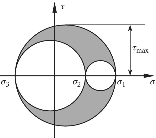
Figure 5.9 Maximum shear stress
In the diagram in figure 5.9, any point (σ, τ) located in the shaded area represents the normal and shear stresses, σn and τn, on a plane through the point. One can note that the maximum shear stress is given by the radius of the largest Mohr’s circle as
The plane on which the shear stress attains maximum bisects the first and third principal stress planes. The normal stress on this plane is given by
5.3 STRAIN
When a solid is subjected to forces, it deforms. A quantitative measure of the deformation is provided by strains. Imagine an infinitesimal line segment in an arbitrary direction at a point in a solid. After deformation, the length of the line segment changes. Strain, specifically the normal strain, in the original direction of the line segment is defined as the change in length divided by the original length. However, this strain will be different in different directions at the same point. In the following, we develop the concept of strain in a three‐dimensional body.
5.3.1 Definition of Strains
Figure 5.10 shows a body before and after deformation. Let the points P, Q, and R in the undeformed body moves to P', Q', and R', respectively, after deformation. The displacement of P can be represented by three displacement components, u, v, and w in the x‐, y‐, and z‐directions. Thus the coordinates of P' are (x + u, y + v, z + w). The functions u(x,y,z), v(x,y,z), and w(x,y,z) are components of a vector field that is referred to as the deformation field or the displacement field. The displacements of point Q will be slightly different from that of P. They can be written as


Figure 5.10 Deformation of line segments
Similarly, displacements of point R are

The coordinates of P, Q, and R before and after deformation are as follows:

Length of the line segment P'Q' can be calculated as
Substituting for the coordinates of P' and Q' from eq. (5.35) we obtain

It may be noted that we have used a two‐term binomial expansion in deriving an approximate expression for the change in length. In this book, we will consider only small deformations such that all deformation gradients are very small compared to unity, that is, ![]() ,
, ![]() . Then we can neglect the higher‐order terms in eq. (5.37) to obtain
. Then we can neglect the higher‐order terms in eq. (5.37) to obtain

Now we invoke the definition of normal strain as the ratio of change in length to original length to derive the expression for strain as
Thus, the normal strain εxx at a point can be defined as the change in length per unit length of an infinitesimally long line segment originally parallel to the x‐axis. Similarly, we can derive normal strains in the y‐ and z‐directions as
The engineering shear strain, say γxy, is defined as the change in the angle between a pair of infinitesimal line segments that were originally parallel to the x‐ and y‐axes. From figure 5.10, the angle between PQ and P'Q' can be derived as
Similarly, the angle between PR and P'R' is
Using the aforementioned definition of shear strain,
Similarly, we can derive shear strains in the yz‐ and zx‐planes as

The shear strains, γxy, γyz, and γzx, are called engineering shear strains. We define tensorial shear strains as

It may be noted that the tensorial shear strains are one half of the corresponding engineering shear strains. It can be shown that the normal strains and the tensorial shear strains transform from one coordinate system to another following tensor transformation rules.
In the general three‐dimensional case, the strain matrix is defined as

As is clear from the definition in eq. (5.45), the strain matrix is symmetric. Like the stress vector, the symmetric strain matrix can be represented as a pseudovector

where γyz, γzx, and γxy are used instead of εyz, εzx, and εxy. The six components of strain completely define the deformation at a point. The normal strain in any arbitrary direction at that point and also the shear strain in any arbitrary plane passing through the point can be calculated using the above strain components, as explained in the following section. Strain is also a tensor and therefore it has properties similar to a stress tensor. For example, the transformation of strain, principal strains, and corresponding principal strain directions can be determined using the procedures we described for stresses.
5.3.2 Transformation of Strain
Let the state of strain at a point be given by the strain matrix [ε]xyz, where the components are expressed in the xyz coordinates shown in figure 5.7. As for the case of stresses, the question again is: What are the components of strain at the same point in a different coordinate system, x′y′z′ (i.e., [ε]x′y′z′)?
Let b1, b2, and b3 be unit vectors along the axes x′, y′, and z′, respectively, represented in xyz coordinates. The strain matrix expressed with respect to the x′y′z′ coordinates system is
which is the same transformation used for stresses in eq. (5.30). It should be emphasized that tensorial shear strains must be used when using the transformation in eq. (5.48).
Let us consider the term ![]() in eq. (5.48). It can be written as
in eq. (5.48). It can be written as
We note that the normal strain in the x'‐direction depends only on the strain tensor and the direction cosines of the x'‐axis. In fact, this relation can be generalized to any arbitrary direction n and written as

Similarly, one can derive the shear strain in a plane containing two mutually perpendicular vectors m and n as

5.3.3 Principal Strains
Strains, like stresses, are second‐order tensors, and therefore one can compute eigenvalues and eigenvectors for a given strain matrix. The eigenvalues are the three principal strains, and the eigenvectors are the corresponding principal strain directions. The principal strain directions represent the directions in which the normal strain εnn in eq. (5.50) takes an extremum value. The maximum and minimum of the three principal strains are the global maximum and minimum, respectively. The three principal planes intersect along the principal strain directions. The shear strain vanishes on the principal strain planes. That is, a pair of infinitesimally small line segments parallel to any two principal directions remain perpendicular to each other after deformation, or, equivalently, the angle between them does not change after deformation. In other words, the shear strain on this plane is equal to zero.
The physical meaning of strains can be explained as follows. Consider an infinitesimal cube of size Δa × Δa × Δa whose sides are parallel to the coordinate axes before deformation. After deformation, the rectangular parallelepiped will become an oblique parallelepiped of size Δa(1+εxx) × Δa (1+εyy) × Δa(1+εzz). The angles between the edges of the parallelepiped will reduce by γxy, γyz, and γzx (see figure 5.11). If the same parallelepiped is oriented such that its edges are parallel to the principal strain directions, then after deformation the parallelepiped will remain as a rectangular parallelepiped, and its dimensions will be Δa(1+ε1) × Δa(1+ε2) × Δa(1+ε3). Since the shear strains in the principal strain planes are zero, the angle between the edges will remain as 90°.

Figure 5.11 Deformation in the principal directions
The principal strain is the extensional strain on a plane, where there is no shear strain. Principal strains and their directions are the eigenvalues and eigenvectors of the following eigenvalue problem:
where n is the eigenvector of matrix ![]() . The above eigenvalue problem has three solutions
. The above eigenvalue problem has three solutions ![]() , and ε3, which are the principal strains.
, and ε3, which are the principal strains.
If the principal strains ε1, ε2, and ε3 are known, then the maximum engineering shear strain γmax can be computed as
where ε1 and ε3 are the maximum and minimum principal strains, respectively.
5.3.4 Stress vs. Strain
Stresses and strains defined in the previous two sections are second‐order tensors and hence share some common properties as shown in table 5.2. When the material is isotropic, which means the material properties are the same in all directions or independent of the coordinates system, the principal stress directions and principal strain directions coincide. If the material is anisotropic, the principal stress and strain directions are in general different. In this textbook, we will focus on isotropic materials only.
Table 5.2 Comparison of stress and strain
| [σ] is a symmetric 3 × 3 matrix | [ε] is a symmetric 3 × 3 matrix |
| Normal stress in the direction n is |
Normal strain in the direction n is |
| Shear stress in a plane containing two mutually perpendicular unit vectors m and n is |
Shear strain in a plane containing two mutually perpendicular unit vectors m and n is |
| Transformation of stresses |
Transformation of strains |
| Three mutually perpendicular principal directions and principal stresses can be computed as eigenvectors and eigenvalues of the stress matrix: |
Three mutually perpendicular principal directions and principal strains can be computed as eigenvectors and eigenvalues of the strain matrix: |
5.4 STRESS–STRAIN RELATIONSHIP
Finding a relationship between the loads acting on a structure and its deflection has been of great interest to scientists since the seventeenth century.5 Robert Hooke, Jacob Bernoulli, and Leonard Euler are some of the pioneers who developed various theories to explain the bending of beams and stretching of bars. Forces applied to a solid create stresses within the body in order to satisfy equilibrium. These stresses also cause deformation or strains. Accumulation of strains over the volume of a body manifests as deflections or gross deformation of the body. Hence, it is clear that a fundamental knowledge of the relationship between stresses and strains is necessary in order to understand the global behavior. Navier tried to explain deformations considering the forces between neighboring particles in a body, as they tend to separate and come closer. Later this approach was abandoned in favor of Cauchy’s stresses and strains. Robert Hooke was the first one to propose the linear uniaxial stress–strain relationship, which states that the stress is proportional to strain. Later the general relationship between the six components of strains and stresses called the generalized Hooke’s law was developed. The generalized Hooke’s law states that each component of stress is a linear combination of strains. It should be mentioned that stress–strain relationships are called phenomenological models or theories as they are based on the commonly observed behavior of materials and verified by experiments. Only recently, with the advancement of computers and computational techniques, behavior of materials based on first principles or fundamental atomistic behavior is being developed. This new field of study is called computational materials and involves techniques such as molecular dynamics simulations and multiscale modeling. Stress–strain relationships are also called constitutive relationships as they describe the constitution of the material.
A cylindrical test specimen is loaded along its axis as shown figure 5.12. This type of loading ensures that the specimen is subjected to a uniaxial state of stress. If the stress–strain relation of the uniaxial tension test in figure 5.12 is plotted, then a typical ductile material may show a behavior as in figure 5.13. The explanation of terms in the figure is summarized in table 5.3.

Figure 5.12 Uniaxial tension test

Figure 5.13 Stress‐strain diagram for a typical ductile material in tension
Table 5.3 Explanations of uniaxial tension test
| Terms | Explanation |
| Proportional limit | The greatest stress for which the stress is still proportional to the strain |
| Elastic limit | The greatest stress that can be applied without resulting in any permanent strain upon unloading |
| Young’s Modulus | Slope of the linear portion of the stress‐strain curve |
| Yield stress | The stress required to produce 0.2% plastic strain |
| Strain hardening | A region where more stress is required to further plastically deform the material |
| Ultimate stress | The maximum stress the material can resist |
| Necking | Cross section of the specimen reduces during deformation |
After the material yields, the shape of the structure permanently changes. Hence, many engineering structures are designed such that the maximum stress is smaller than the yield stress of the material. Under this range of the stress, the stress–strain relation can be approximated by a linear relation.
5.4.1 Linear Elastic Relationship (Generalized Hooke’s Law)
The one‐dimensional stress–strain relationship described in the previous section can be extended to the three‐dimensional state of stress. When the stress–strain relationship is linear, it can be written as
where

Matrix [C] is called the stress–strain matrix, or elasticity matrix. It can be shown that [C] must be a symmetric matrix and hence the number of independent coefficients or elastic constants for an anisotropic material is only 21. Many composite materials, naturally occurring composites such as wood or bone, and man‐made materials such as fiber‐reinforced composites can be modeled as an orthotropic material with nine independent elastic constants. Some composites are transversely isotropic and require only five independent elastic constants. Most materials are isotropic, and for such materials, the 21 constants in the symmetric matrix [C] can be expressed in terms of two independent constants called engineering elastic constants.
For isotropic materials, the relation between stress and strain can be written as:

where E, Young’s modulus, andν, Poisson’s ratio, are the two independent elastic constants, and G is the shear modulus defined by
Note that there are only two independent constants for isotropic materials.
Alternately, stresses can be written as a function of strains by inverting the relations in eq. (5.55), as

The elasticity matrix [C] in eq. (5.54) can be written as

5.4.2 Simplified Laws for Two‐Dimensional Analysis
The general three‐dimensional stress–strain relationship in eq. (5.54) can be simplified for certain special situations that often occur in practice. The two‐dimensional stress–strain relationship can be categorized into three cases: plane stress, plane strain, and axisymmetric.
Most practical structures consist of thin plate‐like components in order to be efficient. Assume a thin plate that is parallel to the xy‐plane. If we assume that the top and bottom surfaces of the plate are not subjected to any significant forces, that is, the plate is subjected to forces in its plane only, in the x‐ and y‐directions, then the transverse stresses (stresses with a z subscript) vanish on the top and bottom surfaces, that is, ![]() on the top and bottom surfaces. If the thickness is much smaller compared to the lateral dimensions of the plate, then we can assume that the aforementioned transverse stresses are approximately zero through the entire thickness. Then the plate is said to be in a state of plane stress parallel to the xy‐plane or normal to the z‐axis.
on the top and bottom surfaces. If the thickness is much smaller compared to the lateral dimensions of the plate, then we can assume that the aforementioned transverse stresses are approximately zero through the entire thickness. Then the plate is said to be in a state of plane stress parallel to the xy‐plane or normal to the z‐axis.
In order to derive the stress–strain relations for the state of plane stress we start with eq. (5.55). We set ![]() on the right‐hand side of the equations to obtain
on the right‐hand side of the equations to obtain

Inverting the above relations, we obtain

Similar to plane stress, one can define a state of plane strain in which strains with a z subscript are all equal to zero. This situation corresponds to a structure whose deformation in the z‐direction is constrained (i.e., w = 0), so that the following relation holds:
Plane strain can also be used if the structure is infinitely long in the z‐direction. The stress–strain relations for the case of plane strain can be derived by starting with eq. (5.54) with the stress–strain matrix [C] in eq. (5.58) and setting the strains with a z subscript, εzz, γxz, and γyz, equal to zero to obtain

The inverse relation is given by

Note that the normal stress σzz is not zero in the plane strain problem but can be calculated from εxx and εyy:
Another class of problems that can be treated as two‐dimensional is the axisymmetric problems where the geometry, the applied loads, and the boundary conditions are all symmetric about an axis. Examples of axisymmetric geometry are a cylinder, a cone, or any geometry that has rotational symmetry about an axis. If the loads and boundary conditions are symmetric about the same axis, then the deformation will be in the radial and axial direction only. That is, there will not be any twisting or rotation about that axis. Therefore, such problems can be treated as two‐dimensional with the displacement vector having only two components. It is convenient to use a cylindrical coordinate system for such problems so that the displacement components, (ur, uz), are the radial and axial components. A two‐dimensional section of this geometry is the domain of analysis. Even though there is no rotation or twisting, there will be strain and stress in the circumferential direction. This component of stress and strain are called hoop stress and hoop strain. The hoop strain occurs whenever there is radial expansion on contraction because any radial displacement would cause the circumference of the object to increase or decrease. In a cylindrical coordinate system, the stress and strain relation can be written as:

This relation can be obtained by dropping the equations for the two out‐of‐plane shear components τrθ and τzθ from the 3D stress‐strain relation in eq. (5.58).
5.5 BOUNDARY VALUE PROBLEMS
5.5.1 Equilibrium Equations
As we discussed earlier, the state of stress at a point is defined by the six stress components, three normal and three shear stresses. These components, in general, vary within the solid. In static problems the stresses can be represented by six functions of the spatial coordinates x, y, and z: σxx(x,y,z), σyy(x,y,z), and so forth. These six functions cannot be arbitrary and must satisfy certain relations called stress equilibrium equations. The functions are also called the stress field in the solid.
Consider the equilibrium of a differential element represented in two dimensions by a square (see figure 5.14) whose center is (x, y) and its sides are dx and dy, respectively. The dimension in the z‐direction is taken as unity. The stresses are assumed to be independent of z, and the solid is in a state of plane stress.

Figure 5.14 Stress variations in infinitesimal components
Equilibrium in the x‐direction yields the following equation:
If the first‐order Taylor series expansion is used to represent stresses on the surfaces of the rectangle in terms of stresses at the center, the first two terms in eq. (5.66) can be approximated by

Similarly, the last two terms can be approximated by

By substituting these two equations into eq. (5.66), we obtain an equilibrium equation in the x‐direction as
Similarly, equilibrium in the y‐direction yields the following equation:
Equations (5.67) and (5.68) are the equilibrium equations for a solid subjected to a two‐dimensional state of stress. We can similarly derive the equations for a three‐dimensional state of stress, by considering the equilibrium of a three‐dimensional differential element to obtain,

Equation (5.69) is obtained by considering force equilibrium in the x‐, y‐, and z‐directions. As has been shown in eq. (5.12), moment equilibrium yields symmetry of the stress matrix.
5.5.2 Traction or Stress Boundary Conditions
While the stress field must satisfy the differential equations of equilibrium in eq. (5.69), there are other conditions the stress field must satisfy on the boundaries of a solid. These are called traction or stress boundary conditions. Consider the surface of a solid subjected to distributed forces such that the tractions in the x‐, y‐ and z‐directions are, tx, ty, and tz, respectively (see figure 5.15). Let the direction cosines of the normal to the surface be nx, ny, and nz. Then the state of stress at a point on the surface of the body must satisfy the boundary conditions shown below:


Figure 5.15 Traction boundary condition of a plane solid
The derivation of the above boundary conditions is similar to those of eq. (5.10).
5.5.3 Boundary Value Problems
Consider an arbitrary body subjected to external forces and displacement constraints as shown in figure 5.16. Our goal is to determine the displacement field u(x,y,z). Once the displacements are determined, strains can be found using the strain displacement relations, that is in eqs. (5.39), (5.40), and (5.45), and then stress field can be determined using the constitutive relations, that is in eq. (5.54). This problem, typical of solid and structural mechanics, is called the elastostatic boundary value problem. Techniques for solving the boundary value problems in two and three dimensions are considered in advanced courses in solid mechanics and theory of elasticity.6 The elasticity problems can be simplified by making certain approximations in the displacement field, for instance, Euler‐Bernoulli beam theory or Kirchhoff plate theory. The finite element method is a numerical method that can solve complex two‐ and three‐dimensional elasticity problems and will be discussed in later chapters.
![A horizontally oriented bar with one end attached to a column. The bar has equation {σ}= [C] {ε}. A downward arrow on the other end represents applied loads.](http://images-20200215.ebookreading.net/2/1/1/9781119078722/9781119078722__introduction-to-finite__9781119078722__images__c05f016.gif)
Figure 5.16 Boundary value problem
In general, solving an elasticity problem involves solving the three equilibrium equations in eq. (5.69) in conjunction with the strain–displacement relations in eqs. (5.39), (5.40), and (5.45) and constitutive relations in eq. (5.54). The boundary conditions also need to be provided in terms of given displacements or prescribed traction forces.
5.5.4 Compatibility Conditions
In the previous section, we talked about the displacement field u(x,y,z). Usually, solutions to the boundary value problems are obtained by trial and error or inverse methods. We first assume a physically suitable displacement field and adjust the terms in the solution to satisfy the equilibrium equations and boundary conditions. More often one needs to start with a physically possible displacement field. In fact, a set of any three nonsingular functions will represent a possible displacement field. Of course, the forces required to produce such a displacement field may be complex and difficult in practice, but still physically possible. However, the same thing cannot be said about the strain field or stress field. That is, one cannot choose six arbitrary functions in spatial coordinates and claim the set to be a possible strain field. The particular strain field may not be physically possible. For example, a valid strain field should not create a discontinuous deformation or overlapping of certain points. The six strain functions must satisfy three relations called compatibility equations. The derivation of the three‐dimensional compatibility equation is beyond the scope of this book. The interested reader is referred to more advanced elasticity books, such as Timoshenko.7 For two‐dimensional (plane) problems, the compatibility equation is given as

5.6 PRINCIPLE OF MINIMUM POTENTIAL ENERGY FOR PLANE SOLIDS
There are different methods to solve for the boundary value problems in the previous section. In this section, the principle of minimum potential energy that is similar to the beam‐bending problem in chapter 3 is derived for plane solids. The principle will be used to derive the finite element equations for different elements in the next chapter.
5.6.1 Strain Energy in a Plane Solid
Consider a plane elastic solid as illustrated in figure 5.18. The strain energy is a form of energy that is stored in the solid due to the elastic deformation. Formally, it can be defined as

where h is the thickness of the plane solid (h = 1 for plane strain) and [C] = [Cσ] for plane stress and [C] = [Cε] for plane strain. Since stress and strain are constant throughout the thickness, the volume integral is converted into the area integral by multiplying by the thickness in the second relation in eq. (5.72). The linear elastic relation in eq. (5.54) has been used in the last relation.

Figure 5.18 A plane solid under the distributed load {Tx, Ty} on the traction boundary ST
5.6.2 Potential Energy of Applied Loads
When a force acting on a body moves through a small distance, it loses its potential to do additional work, and hence its potential energy is given by the negative of the product of the force and corresponding displacement. For example, when concentrated forces are applied to the solid, the potential energy becomes

where Fi is the force in the i‐th DOF, qi is the displacement in the direction of the force, and ND is the total number of concentrated forces acting on the body. The negative sign indicates that the potential energy decreases as the force has expended some energy performing the work given by the product of force and corresponding displacement.
When distributed forces, such as a pressure load, act on the edge of a body, the summation sign in the above expression is replaced by integration over the edge of the body as shown below:

where Tx and Ty are the components of applied surface forces in the x‐ and y‐direction, respectively. In the finite element discretization, the vector of displacements, {u}, is approximated by shape functions and nodal DOFs {q}. Therefore, the potential energy of the applied loads is a function of nodal DOFs {q} after discretization by finite elements.
If body forces (forces distributed over the volume) are present, work done by these forces can be computed in a similar manner. The gravitational force is an example of body force. In this case, integration should be performed over the volume. We will discuss this further when we derive the finite element equations.
5.6.3 Principle of Minimum Potential Energy
As with the beam problem, the potential energy is defined as the sum of the strain energy and the potential energy of applied loads:
where U is the strain energy and V is the potential energy of applied loads. The principle of minimum total potential energy states that of all possible displacement configurations of a solid/structure, the equilibrium configuration corresponds to the minimum total potential energy. That is, at equilibrium, we have

where q1, q2, …, qN are nodal DOFs (i.e., displacements) that define the deformed configuration of the body. In finite element analysis, the deformation of the body is defined in terms of the displacements of the nodes. In the next chapter, we will use the principle of minimum total potential energy to derive finite element equations for different types of elements.
5.7 FAILURE THEORIES
In the previous section, we introduced the concept of stress, strain, and the relationship between stresses and strains. We also discussed the failure of materials under a uniaxial state of stress. Failure of engineering materials can be broadly classified into ductile and brittle failure. Most metals are ductile and fail due to yielding. Hence, the yield strength characterizes their failure. Ceramics and some polymers are brittle and rupture or fracture when the stress exceeds certain maximum value. Their stress–strain behavior is linear up to the point of failure and they fail abruptly.
The stress required to break the atomic bond and separate the atoms is called the theoretical strength of the material. It can be shown that the theoretical strength is approximately equal to E/3 where E is Young’s modulus.8 However, most materials fail at a stress about one‐hundredth or even one‐thousandth of the theoretical strength. For example, the theoretical strength of aluminum is about 22 GPa. However, the yield strength of aluminum is in the order of 100 MPa, which is 1/220 of the theoretical strength. This enormous discrepancy could be explained as follows.
In ductile materials, yielding occurs not due to separation of atoms but due to sliding of atoms (movement of dislocations) as depicted in figure 5.19. Thus, the stress or energy required for yielding is much less than that required for separating the atomic planes. Hence, in a ductile material, the maximum shear stress causes yielding of the material.

Figure 5.19 Material failure due to relative sliding of atomic planes
In brittle materials, the failure or rupture still occurs due to the separation of atomic planes. However, the high value of stress required is provided locally by stress concentration caused by small pre‐existing cracks or flaws in the material. The stress concentration factors can be in the order of 100 to 1,000. That is, the applied stress is amplified by the enormous amount due to the presence of cracks, and it is sufficient to separate the atoms. When this process becomes unstable, the material separates over a large area causing brittle failure of the material.
Although research is underway not only to explain but also quantify the strength of materials in terms of its atomic structure and properties, it is still not practical to design machines and structures based on such atomistic models. Hence, we resort to phenomenological failure theories, which are based on observations and testing over a period. The purpose of failure theories is to extend the strength values obtained from uniaxial tests to multiaxial states of stress that exist in practical structures. It is not practical to test a material under all possible combinations of stress states. In the following, we describe some well‐established phenomenological failure theories for both ductile and brittle materials.
5.7.1 Strain Energy
When a force is applied to a solid, it deforms. Then, we can say that work is done on the solid, which is proportional to the force and deformation. The work done by the applied force is stored in the solid as potential energy, which is called the strain energy. The strain energy in the solid may not be distributed uniformly throughout the solid. We introduce the concept of strain energy density, which is strain energy per unit volume, and we denote it by U0. Then the strain energy in the body can be obtained by integration as follows:
where the integration is performed over the volume V of the solid. In the case of uniaxial stress state, the strain energy density is equal to the area under the stress–strain curve (see figure 5.20). Thus, it can be written as

Figure 5.20 Stress–strain curve and the strain energy
For the general 3‐D case the strain energy density is expressed as
If the material is elastic, then the strain energy can be completely recovered by unloading the body.
The strain energy density in eq. (5.79) can be further simplified. Consider a coordinate system that is parallel to the principal stress directions. In this coordinate system, no shear components exist. Extending eq. (5.79) to this stress states yields
From section 5.3, we know that stresses and strains are related through the linear elastic relationship. For example, in case of principal stresses and strains,

Substituting from eq. (5.81) into eq. (5.80), we can write the strain energy density in terms of principal stresses as
The strain energy density can be thought of as consisting of two components: one due to dilation or change in volume and the other due to distortion or change in shape. The former is called dilatational strain energy and the latter, distortional energy. Many experiments have shown that ductile materials can be hydrostatically stressed to levels beyond their ultimate strength in compression without failure. This is because the hydrostatic state of stress reduces the volume of the specimen without changing its shape.
5.7.2 Decomposition of Strain Energy
The strain energy density at a point in a solid can be divided into two parts: dilatational strain energy density, Uh, that is due to change in volume, and distortional strain energy density, Ud, that is responsible for the change in shape. In order to compute these components, we divide the stress matrix also into similar components, dilatational stress matrix, σh, and deviatoric stress matrix, σd. For convenience, we will use the stress components with respect to the principal stress coordinates. Then the aforementioned stress components can be derived as follows:

The dilatational component σh is defined as
which is also called the volumetric stress. Note that 3σh is the first invariant I1 of the stress matrix in eq. (5.20). Thus, it is independent of the coordinate system. Note that σh is a state of hydrostatic stress and hence the subscript h is used to denote the dilatational stress component as well as dilatational energy density
The dilatational energy density can be obtained by substituting the stress components of the hydrostatic stress state in eq. (5.84) into the expression for strain energy density in eq. (5.82),

and using the relation in eq. (5.84),

The distortion part of the strain energy is now found by subtracting eq. (5.86) from eq. (5.82), as

It is customary to write Ud in terms of an equivalent stress called von Mises stress, σVM, as
The von Mises stress is defined in terms of principal stresses as

5.7.3 Distortion Energy Theory (von Mises)
According to von Mises’s theory, a ductile solid will yield when the distortion energy density reaches a critical value for that material. Since this should be true for the uniaxial stress state also, the critical value of the distortional energy can be estimated from the uniaxial test. At the instance of yielding in a uniaxial tensile test, the state of stress in terms of principal stress is given by σ1 = σY (yield stress) and σ2 = σ3 = 0. The distortion energy density associated with yielding is
Thus, the energy density given in eq. (5.90) is the critical value of the distortional energy density for the material. Then according to von Mises’s failure criterion, the material under multiaxial loading will yield when the distortional energy is equal to or greater than the critical value for the material:
Thus, the distortion energy theory states that material yields when the von Mises stress exceeds the yield stress obtained in a uniaxial tensile test.
The von Mises stress in eq. (5.87) can be rewritten in terms of stress components as

For a two‐dimensional plane stress state, σ3 = 0, the von Mises stress can be defined in terms of principal stresses as
and in terms of general stress components as
The two‐dimensional distortion energy equation in eq. (5.94) becomes an ellipse when plotted on the σ1‐σ2 plane as shown in figure 5.21. The interior of this ellipse defines the region of combined biaxial stress where the material is safe against yielding under static loading.

Figure 5.21 Failure envelope of the distortion energy theory
Consider a situation in which only a shear stress exists, such that σx = σy = 0, and τxy = τ. For this stress state, the principal stresses are σ1 = –σ3 = τ and σ2 = 0. On the σ1‐σ3 plane, this pure shear state is represented as a straight line through the origin at –45° as shown in figure 5.21. The line intersects the von Mises failure envelope at two points, A and B. The magnitude of σ1 and σ2 at these points can be found from eq. (5.93) as
Thus, in a pure shear stress state, the material yields when the shear stress reaches 0.577σY. This value will be compared to the maximum shear stress theory described below.
5.7.4 Maximum Shear Stress Theory (Tresca)
According to the maximum shear stress theory, the material yields when the maximum shear stress at a point equals the critical shear stress value for that material. Since this should be true for a uniaxial stress state, we can use the results from uniaxial tension test to determine the maximum allowable shear stress. The stress state in a tensile specimen at the point of yielding is given by σ1 = σY, σ2 = σ3 = 0. The maximum shear stress is calculated as
This value of maximum shear stress is also called the yield shear stress of the material and is denoted by τY. Note that τY = σY/2. Thus, Tresca’s yield criterion is that yielding will occur in a material when the maximum shear stress equals the yield shear strength, τY, of the material.
The hexagon in figure 5.22 represents the two‐dimensional failure envelope according to maximum shear stress theory. The ellipse corresponding to von Mises’s theory is also shown in the same figure. The hexagon is inscribed within the ellipse and contacts it at six vertices. Combinations of principal stresses σ1 and σ3 that lie within this hexagon are considered safe based on the maximum shear stress theory, and failure is considered to occur when the combined stress state reaches the hexagonal boundary. This is obviously more conservative failure theory than distortion energy theory as it is contained within the latter. In the pure shear stress state, the shear stress at points C and D correspond to 0.5σY, which is smaller than 0.577σY, the failure point according to the distortion energy theory.

Figure 5.22 Failure envelope of the maximum shear stress theory
5.7.5 Maximum Principal Stress Theory (Rankine)
According to the maximum principal stress theory, a brittle material ruptures when the maximum principal stress in the specimen reaches some limiting value for the material. Again, this critical value can be inferred as the tensile strength measured using a uniaxial tension test. In practice, this theory is simple but can only be used for brittle materials. Some practitioners have modified this theory for ductile materials as
where σ1 is the maximum principal stress, and σU is the ultimate strength described in table 5.3. Figure 5.23 shows the failure envelope based on the maximum principal stress theory. Note that the failure envelopes in the first and third quadrants are coincident with those of the maximum shear stress theory and contained within the distortion energy theory. However, the envelopes in the second and fourth quadrants are well outside of the other two theories. Hence, the maximum principal stress theory is not considered suitable for ductile materials. However, it can be used to predict failure in brittle materials.

Figure 5.23 Failure envelope of the maximum principal stress theory
5.8 SAFETY FACTOR
One can notice that the all aforementioned failure theories are of the form:
The term on the left‐hand side of a failure criterion depends on the state of stress at a point. Various stress analysis methods, including the finite element method discussed in this book, are used to evaluate the stress term. The right‐hand side of the equation is a material property usually determined from material tests. There are many uncertainties in calculating the state of stress at a point. These include uncertainties in the loads, material properties such as Young’s modulus, dimensions and geometry of the solid, and so forth. Similarly, there are uncertainties in the strength of a material depending on the tests used to measure the strength, manufacturing process, and so forth. In order to account for the uncertainties, engineers use a factor of safety in the design of a solid or structural component. Thus, the failure criteria are modified as:
where N is the safety factor. That is, we assume the stress is N times the calculated or estimated state of stress. Another interpretation is that the strength is reduced by a factor N to account for uncertainties. Thus, the space of allowable stresses is contained well within the failure envelope shown in figure 5.23. For example, the safety factor in the von Mises theory is defined as
In many engineering applications, N is in the range of 1.1–1.5.
The safety factor in the maximum shear stress theory is defined as
It can be shown that for any two‐dimensional loading, ![]() .
.

5.9 EXERCISES
- Answer the following descriptive questions.
- How can the sign of Cartesian components of stress be determined?
- When the three principal stresses are identical, that is, σ1 = σ2 = σ3 = σ, what are the principal directions?
- When the only nonzero stress components are σxx = σyy = σzz = σ, will n = {1, 2, 3}T be a principal direction?
- When γxy = 150 MPa is the only nonzero strain component, what are the three principal strains?
- For a 2D model, when is it more appropriate to use plane stress elements rather than plane strain elements? Give examples of both.
- When can a structure be modeled using axisymmetric elements? Give two examples.
- If a thin rectangular plate is rigidly held along all its edges and a transverse load is applied normal to the plate, is it appropriate to model it as 2D (plane stress or plane strain)? Explain why or why not.
- In the real world, all structures are 3D. Why is it then not appropriate to always use 3D elements for all structures? Explain this for the case of a frame‐like structure.
- A vertical force F is applied to a two‐bar truss as shown in the figure. Let the cross‐sectional areas of trusses 1 and 2 be A1 and A2, respectively. Determine the area ratio A1/A2 in order to have the same magnitude of stresses in both members.

- The stress matrix at a point P is given below. The direction cosines of the normal n to a plane that passes through P have the ratio nx:ny:nz = 3:4:12. Determine: (a) the traction vector T(n); (b) the magnitude T of T(n); (c) the normal stress σn; (d) the shear stress τn; and (e) the angle between T(n) and n. Hint: Use
 .
.
- At a point P in a body, Cartesian stress components are given by σxx = 80 MPa, σyy = −40 MPa, σzz = −40 MPa, and τxy = τyz = τzx = 80 MPa. Determine the traction vector and its normal component and shear component on a plane that is equally inclined to all three axes.
Hint: When a plane is equally inclined to all the three coordinate axes, the direction cosines of the normal are equal to each other.
- If σxx = 90 MPa, σyy = −45 MPa, τxy = 30 MPa, and σzz = τxz = τyz = 0, compute the surface traction T(n) on the plane shown in the figure, which makes an angle of θ = 40° with the vertical axis. What are the normal and shear components of stress on this plane?

- Find the principal stresses and the orientation of the principal axes of stresses for the following cases of plane stress.
- σxx = 40 MPa, σyy = 0 MPa, τxy = 80 MPa
- σxx = 140 MPa, σyy = 20 MPa, τxy = −60 MPa
- σxx = −120 MPa, σyy = 50 MPa, τxy = 100 MPa
- If the minimum principal stress is −7 MPa, find σxx and the angle that the principal stress axes make with the xy axes for the case of plane stress illustrated.

- Determine the principal stresses and their associated directions, when the stress matrix at a point is given by

- Let an x′y′z′ coordinate system be defined using the three principal directions obtained from problem 8. Determine the transformed stress matrix [σ]x′y′z′ in the new coordinate system.
- For the stress matrix below, the two principal stresses are given as σ3 = −3 and σ1 = 2, respectively. In addition, two principal directions corresponding to the two principal stresses are also given below.

- What are the normal and shear stresses on the plane whose normal vector is parallel to (2, 1, 2)?
- Calculate the principal stress σ2 and the principal direction n2.
- Write the stress matrix in the new coordinate system that is aligned with n1, n2, and n3.
- With respect to the coordinate system xyz, the state of stress at a point P in a solid is:


- m1, m2 and m3 are three mutually perpendicular vectors such that m1 makes 45° with both the x‐ and y‐axis and m3 is aligned with the z‐axis. Compute the normal stresses on planes normal to m1, m2, and m3.
- Compute two components of shear stress on the plane normal to m1 in the directions m2 and m3.
- Is the vector n = {0, 1, 1}T a principal direction of stress? Explain. What is the normal stress in the direction n?
- Draw an infinitesimal cube with faces normal to m1, m2, and m3 and display the stresses on the positive faces of this cube.
- Express the state of stress at the point P with respect to the x′y′z′ coordinates system that is aligned with the vectors m1, m2 and m3?
- What are the principal stress and principal directions of stress at the point P with respect to the x′y′z′ coordinate system? Explain.
- Compute the maximum shear stress at point P. Which plane(s) does this maximum shear stress act on?
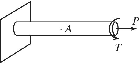
- A solid shaft of diameter d = 5 cm as shown in the figure is subjected to tensile force P = 13,000 N and a torque T = 6,000 N⋅cm. At point A on the surface, what is the state of stress (write in matrix form), the principal stresses, and the maximum shear stress? Show the coordinate system you are using.
- The solid shaft in problem 12 has diameter d = 10 cm and is subjected to tensile force P = 80,000 N and a torque T = 5,000 N⋅cm. Assume that the yield stress of the material of the shaft is σy = 200 MPa.
- Compute the state of stress at a potential point of failure.
- Based on the Maximum Shear stress theory (Tresca’s law) will this shaft fail? What is the safety factor?
- If the displacement field is given by

- Write down the 3 × 3 strain matrix.
- What is the normal strain component in the direction of (1,1,1) at point (1,–3,1)?
- If the displacement field is given bywhere k is a constant,

- Write down the strain matrix.
- What is the normal strain in the direction of n = {1, 1, 1}T?
- Consider the following displacement field in a plane solid:

- Compute the infinitesimal strain components εx, εy, and γxy. Is this a state of uniform strain?
- Determine the principal strains and their corresponding directions. Express the principal strain directions in terms of the angles (in degrees) the directions make with the x‐axis.
- What is the normal strain at (x,y) in a direction 45o to the x‐axis?
- Draw a 2‐inch × 2‐inch square OABC on the engineering paper. The coordinates of O are (0, 0) and those of B are (2, 2). Using the displacement field in problem 16, determine the u and v displacements of the corners of the square. Let the deformed square be denoted as O'A'B'C'.
- Determine the change in lengths of OA and OC. Relate the changes to the strain components.
- Determine the change in
 . Relate the change to the shear strain.
 - Determine the change in length in the diagonal OB. How is it related to the strain(s)?
- Show that the relative change in the area of the square (change in area/original area) is given by ΔA/A = εxx + εyy = ε1 + ε2.
Hint: You can use the old‐fashioned method of using set‐squares (triangles) and protractor or use a spreadsheet to do the calculations. Place the origin somewhere in the bottom middle of the paper so that you have enough room to the left of the origin.
- Draw a 2‐inch × 2‐inch square OPQR such that OP makes +73o to the x‐axis. Repeat questions (a) through (d) in problem 17 for OPQR. Give physical interpretations to your results.
Note: The principal strains and the principal strain directions are given by:
- For steel, the following material data are applicable: Young’s modulus E = 207 GPa and shear modulus G = 80 GPa. For the strain matrix at a point shown below, determine the symmetric 3 × 3 stress matrix.

- Strain at a point is such that εxx = εyy = 0, εzz = −0.001, εxy = 0.006, and εxz = εyz = 0. Note: You need not solve the eigenvalue problem for this question.
- Show that n1 = i + j and n2 = −i + j are principal directions of strain at this point.
- What is the third principal direction?
- Compute the three principal strains.
- Derive the stress–strain relationship in eq. (5.60) from eq. (5.55) and the plane stress conditions.
- A thin plate of width b, thickness t, and length L is placed between two frictionless rigid walls a distance b apart and is acted on by an axial force P. The material properties are Young’s modulus E and Poisson’s ratio ν.
- Find the stress and strain components in the xyz coordinate system.
- Find the displacement field.

- A solid with Young’s modulus E =70 GPa and Poisson’s ratio = 0.3 is in a state of plane strain parallel to the xy‐plane. The in‐plane strain components are measured as: εxx = 0.007, εyy = −0.008, and γxy = 0.02.
- Compute the principal strains and corresponding principal strain directions.
- Compute the stresses, including σzz, corresponding to the above strains.
- Determine the principal stresses and corresponding principal stress directions. Are the principal stress and principal strain directions the same?
- Show the principal stresses could have been obtained from the principal strains using the stress‐strain relations.
- Compute the strain energy density using the stress and strain components in the xy‐coordinate system.
- Compute the strain energy density using the principal stresses and principal strains.
- Assume that the solid in problem 23 is under a state of plane stress. Repeat (b) through (f).
- A strain rosette consisting of three strain gauges was used to measure the strains at a point in a thin‐walled plate. The measured strains in the three gauges are: εA = 0.001, εB = −0.0006, and εC = 0.0007. Note that gauge C is at 45° with respect to the x‐axis. Assume the plane stress state.
- Determine the complete state of strains and stresses (all 6 components) at that point. Assume E = 70 GPa, and ν = 0.3.
- What are the principal strains and their directions?
- What are the principal stresses and their directions?
- Show that the principal strains and stresses satisfy the stress‐strain relations.

- A strain rosette consisting of three strain gauges was used to measure the strains at a point in a thin‐walled plate. The measured strains in the three gauges are: εA = 0.016, εB = 0.004, and εC = 0.016. Determine the complete state of strains and stresses (all six components) at that point. Assume E = 100 GPa, and ν = 0.3.

- A strain rosette consisting of three strain gauges was used to measure the strains at a point in a thin plate of dimensions 100 × 20 × 1 mm. The measured strains in the three gauges are: εA = 0.008, εB = 0.002, and εC = 0.008. Assume E = 100 GPa, and ν = 0.3.
- Assuming the plate is in a state of plane stress, determine the complete state of strains and stresses (all six components) at that point.
- Assuming the state of stress is uniform, calculate the strain energy stored in the plate.

- The figure below illustrates a thin plate of thickness t. An approximate displacement field, which accounts for displacements due to the weight of the plate, is given by

- Determine the corresponding plane stress field.
- Qualitatively draw the deformed shape of the plate.

- The stress matrix at a particular point in a body isDetermine the corresponding strain if E = 20 × 1010 Pa and ν = 0.3.

- For a plane stress problem, the strain components in the xy‐plane at a point P are computed as:

- Compute the state of stress at this point if Young’s modulus E = 2×10¹¹ Pa and Poisson’s ratio ν = 0.3.
- What is the normal strain in the z‐direction?
- Compute the normal strain in the direction of n = {1, 1, 1}T.
- The state of strain at a point P in a structure is

- Compute the extensional strain in the direction
 .
. - If
 and
and  are principal directions, compute the three principal strains at this point.
 - Compute the principal stresses at this point if Young's Modulus E = 2x10¹¹ Pa and Poisson's ratio ν = 0.3. (Use principal strains from part (b)).
- Can the state of stress at this point be described as plane stress? Explain.
- Compute the strain energy density at the point P.
- If the yield stress of the material of the plate is σy = 2 × 10⁸ Pa, has this plate undergone plastic deformation due to the applied strain? Use maximum shear stress criterion (Tresca’s law) to answer this question.
- Compute the extensional strain in the direction
- The state of stress at a point is given by

- Determine the strains using Young’s modulus of 100 GPa and Poisson’s ratio of 0.25.
- Compute the strain energy density using these stresses and strains.
- Calculate the principal stresses.
- Calculate the principal strains from the strains calculated in (a).
- Show that the principal stresses and principal strains satisfy the constitutive relations.
- Calculate the strain energy density using the principal stresses and strains.
- Consider the state of stress in problem 32. The yield strength of the material is 100 MPa. Determine the safety factors according to: (a) maximum principal stress criterion, (b) Tresca criterion, and (c) von Mises criterion.
- A thin‐walled tube is subject to a torque T. The only nonzero stress component is the shear stress τxy, which is given by τxy = 10,000 T (Pa), where T is the torque in N.m. When the yield strength σY = 300 MPa and the safety factor N = 2, calculate the maximum torque that can be applied using:
- maximum principal stress criterion (Rankine);
- maximum shear stress criterion (Tresca); and
- distortion energy criterion (Von Mises).
- A thin‐walled cylindrical pressure vessel with closed ends is subjected to an internal pressure p = 100 psi and also a torque T about its axis of symmetry. Determine T that will cause yielding according to von Mises’ yield criterion. The design requires a safety factor of 2. The nominal diameter D of the pressure vessel = 20 inch, wall thickness t = 0.1 in., the yield strength of the material = 30 ksi. (1 ksi = 1000 psi). Stresses in a thin‐walled cylinder are: longitudinal stress σl, hoop stress σh, and shear stress τ due to torsion. They are given by

- A cold‐rolled steel shaft is used to transmit 60 kW at 500 rpm from a motor. What should be the diameter of the shaft, if the shaft is 6 m long and is simply supported at both ends? The shaft also experiences bending due to a distributed transverse load of 200 N/m. Ignore bending due to the weight of the shaft. Use a safety factor of 2. The tensile yield limit is 280 MPa. Find the diameter using both maximum shear stress theory and von Mises’ criterion for failure.
- For the stress matrix below, the two principal stresses are given as σ1 = 2 and σ3 = –3, respectively. In addition, two principal directions corresponding to the two principal stresses are also given below. The yield stress of the structure is given as σY = 4.5.

- Calculate the safety factor based on the maximum shear stress theory and determine whether the structure is safe.
- Calculate the safety factor based on the distortion energy theory and determine whether the structure is safe or not.
- The figure below shows a round shaft of diameter 1.5 in. loaded by a bending moment Mz = 5,000 lb.·in., a torque T = 8,000 lb.·in., and an axial tensile force N = 6,000 lb. If the material is ductile with the yielding stress σY = 40,000 psi, determine the safety factor corresponding to yield using (a) the maximum shear stress theory and (b) the maximum distortion energy theory.

- A 20‐mm diameter rod made of a ductile material with a yield strength of 350 MPa is subject to a torque of T = 100 N·m and a bending moment of M = 150 N·m. An axial tensile force P is then gradually applied. What is the value of the axial force when yielding of the rod occurs? Solve the problem two ways using (a) the maximum shear stress theory and (b) the maximum distortional energy theory.

- A circular shaft of radius r in the figure has a moment of inertia I and polar moment of inertia J. The shaft is under torsion Tz in the positive z‐axis and bending moment Mx in the positive x‐axis. The material is mild steel with a yield strength of 2.8 MPa. Use only the given coordinate system for your calculations.
- If Tz and Mx are gradually increased, which point (or points) will fail first among four points (A, B, C, and D)? Identify all.
- Construct the stress matrix [σ]A at point A in xyz‐coordinates in terms of the given parameters (i.e., Tz, Mx, I, J, and r).
- Calculate three principal stresses at point B in terms of the given parameters.
- When the principal stresses at point C are σ1 = 1, σ2 = 0, and σ3 = −2 MPa, calculate safety factors (1) from maximum shear stress theory and (2) from distortion energy theory.

- A rectangular plastic specimen of size 100 × 100 × 10 mm3 is placed in a rectangular metal cavity. The dimensions of the cavity are 101 × 101 × 9 mm3. The plastic is compressed by a rigid punch until it is completely inside the cavity. Due to Poisson effect, the plastic also expands in the x‐ and y‐direction and fill the cavity. Calculate all stress and strain components and the force exerted by the punch. Assume there is no friction between all contacting surfaces. The metal cavity is rigid. Elastic constants of the plastic are: E = 10 GPa, ν = 0.3.

- Repeat problem 41 with elastic constants of the plastic as E = 10 GPa and ν = 0.485.
- Repeat problem 41 with the specimen of size 100 × 100 × 10 mm3 and the dimensions of the cavity 104 × 104 × 9 mm3. Elastic constants of the plastic are: E = 10 GPa, ν = 0.3.