
Chapter 7
Isoparametric Finite Elements
7.1 INTRODUCTION
The shape functions for triangular and rectangular elements in chapter 6 are derived in the global coordinates and are dependent on the nodal coordinates of the element. Therefore, different elements have different shape functions. Knowing that hundreds of thousands of elements are often used in solving practical problems, evaluating the shape functions for individual elements might be laborious and computationally inefficient. In addition, deriving the shape functions for quadrilaterals in global coordinates is difficult as compared to rectangular elements. It is often convenient to use local coordinate systems for interpolating the field variables such as displacement or temperature fields because the shape functions are easier to derive and have simpler expressions. This involves a change of variables from the physical (x,y) or (x,y,z) coordinates to parametric (s,t) or (r,s,t) coordinates. Isoparametric elements use a parametric coordinate system that transforms the elements by scaling and deforming it. The domain in the parametric coordinate system is often referred to as the parametric space, as opposed to the space occupied by the element in the global coordinate system, which is the physical space. A mapping is established between the physical and parametric spaces. The advantage of using this approach is that more complex‐shaped elements can be constructed such as quadrilateral and hexahedral elements. In addition, since shape functions are calculated in the parametric space, and since all elements are mapped into the same parametric space, all elements in different geometry share the same shape functions. Only the mapping from individual elements to the parametric space is different for different elements.
In this chapter, we introduce the concept of isoparametric elements first with one‐dimensional elements. The linear one‐dimensional elements are very similar to the elements we have already seen in the previous chapters. For higher‐order elements such as quadratic or even cubic elements, the isoparametric element formulation has several advantages. The shape functions of these elements are much easier to derive when parametric coordinates are used. Systematic methods for deriving these shape functions using Lagrange interpolation techniques are available that are also presented in section 7.2 for one‐dimensional elements and in section 7.3 for two‐dimensional elements. Even though the isoparametric formulation simplifies the element geometry in the parametric space, it is still difficult to analytically integrate over the geometry to compute a stiffness matrix or load vector, and therefore numerical integration is needed. Another advantage of isoparametric element is that it is convenient to apply numerical integration methods. In finite element analysis, the method of Gauss quadrature is predominantly used for numerical integration to evaluate the stiffness matrix or load vector, which will be discussed in 7.4. Using the isoparametric formulation, higher‐order quadrilateral elements and triangular elements will be derived and discussed in sections 7.5 and 7.6. Although most important theoretical and numerical aspects of the finite element method can be illustrated using one‐ and two‐dimensional problems, some three‐dimensional elements are introduced in section 7.7 to demonstrate the complexity of the formulation. Section 7.8 discusses some modeling issue for practical problems, followed by three projects in section 7.9.
7.2 ONE‐DIMENSIONAL ISOPARAMETRIC ELEMENTS
7.2.1 2‐Node Linear Isoparametric Element
A one‐dimensional 2‐node linear element is used here to introduce the concept of an isoparametric element. Figure 7.1 shows a one‐dimensional domain of length L where the physical coordinate x has a domain of ![]() . This domain can be the one‐dimensional bar in chapter 1 or one‐dimensional heat transfer in a rod in chapter 4. The domain is discretized by NEL number of elements. An element e in this domain is shown, which has nodal coordinate of xi and xj at nodes i and j respectively. This element is mapped to a reference element, which is defined using the reference coordinate s. The reference element has a domain of
. This domain can be the one‐dimensional bar in chapter 1 or one‐dimensional heat transfer in a rod in chapter 4. The domain is discretized by NEL number of elements. An element e in this domain is shown, which has nodal coordinate of xi and xj at nodes i and j respectively. This element is mapped to a reference element, which is defined using the reference coordinate s. The reference element has a domain of ![]() . The reference element has two nodes. Node i in physical element is mapped to node 1 in the reference element, and node j to node 2. Note that the physical element has a length
. The reference element has two nodes. Node i in physical element is mapped to node 1 in the reference element, and node j to node 2. Note that the physical element has a length ![]() , while the reference element has a fixed length of 2.
, while the reference element has a fixed length of 2.
We need a mapping function x(s), which defines the relation between these two coordinates such that ![]() and
and ![]() . For isoparametric elements, the shape functions used for interpolation are also used for defining this mapping function. The shape functions are first derived in the reference element as a function of the parameter s. For this 2‐node linear element, we can assume that the shape functions are in the form of
. For isoparametric elements, the shape functions used for interpolation are also used for defining this mapping function. The shape functions are first derived in the reference element as a function of the parameter s. For this 2‐node linear element, we can assume that the shape functions are in the form of ![]() .
.

Figure 7.1 One‐dimensional 2‐node linear isoparametric element
The shape functions must satisfy the Kronecker’s delta condition, that is,

Using this condition for node 1, we get the following two equations to determine N1(s)

Solving these two equations, we get ![]() and
and ![]() . Substituting this into N1(s), we get,
. Substituting this into N1(s), we get,
Similarly, using eq. (7.1) for node 2, we can solve for the second shape function as,
These shape functions can be used for interpolation as we have done in the previous chapters, but this yields an interpolation in parametric space. For example, if we use this element for heat conduction analysis, the temperature within the element can be interpolated using nodal temperature as

Note that the temperature is now a function of the parameter s rather than the physical coordinate x. Therefore we need a mapping function that establishes the relation between x and s. In isoparametric elements, this mapping function is constructed using the same shape functions as
It can be easily verified that this mapping satisfies the condition that at node 1, ![]() ,
, ![]() and similarly, at node 2,
and similarly, at node 2, ![]() .
.
As expected we get the same stiffness matrix that we obtained earlier when we were not using the isoparametric formulation. Clearly, the element is the same whether we use an isoparametric formulation or not. But by changing the variable from the physical coordinate to the reference coordinate with a more convenient domain, it becomes a little easier to derive the shape functions and to carry out the integration for evaluating the stiffness matrix. This advantage is all the more critical for more complex‐shaped elements such as quadrilaterals as well as higher‐order elements, where it is much more difficult to derive the shape functions in terms of the global coordinates.
7.2.2 Quadratic 3‐Node Isoparametric Element
In the previous section, we saw that if the element has 2‐nodes, then we can fit a straight line between the values at the two nodes to obtain a linear interpolation. This is because we had two nodal values to fit a function, and a linear function has two unknown coefficients. If we need a higher‐order element, we need more nodes in the element or have more variables per node. A quadratic element can be constructed if the element has three nodes so that we can fit a parabolic curve between the three nodal values.
For the physical element, the element connectivity is given as i‐j‐k, where node i and j are two end nodes and node k is the one in between. In the finite element community, it is customary that node numbers are given to the corner nodes first followed by nodes on the edges. Node k may not be located at the center of the element in the global coordinates even though it is at the center in the parametric space. However, if the node is not centrally placed in the global coordinates, then the mapping is distorted as we shall see in later discussion. For the reference element, the element connectivity is given as 1‐2‐3, where node 1 is at ![]() , node at
, node at ![]() , and node 3 at
, and node 3 at ![]() .
.

We will assume that the quantity we are interpolating (say, the temperature) and the shape functions are quadratic polynomials, as
That means, the shape functions are also a quadratic polynomial, as
Again, one could use the Kronecker’s delta condition to derive the shape functions. For the first shape function

Solving these equations, we get ![]() ,
, ![]() , and
, and ![]() . Similarly, we can solve for the other shape functions. Therefore, three shape functions for a quadratic element can be obtained as
. Similarly, we can solve for the other shape functions. Therefore, three shape functions for a quadratic element can be obtained as

The mapping function for the element is again constructed using the same shape functions in all isoparametric elements.
We could have used the mapping function we derived for the 2‐node linear element here. That is, the displacement is interpolated using quadratic shape functions, while the geometry is interpolated using linear shape functions. But then the element would not be isoparametric. Instead, it would be a sub‐parametric element because the mapping function is of a lower order than the interpolation. Similarly, one can construct super‐parametric elements that use a higher‐order mapping function than the order of the interpolation used for the element. So the term isoparametric comes from the notion of using the same shape functions to create both the mapping and the interpolation.

Figure 7.3 Regular versus irregular quadratic element

Figure 7.4 Mapping and interpolation for the regular element

Figure 7.5 Irregular versus irregular quadratic element

Figure 7.6 1‐D heat conduction model using 3‐node elements
Table 7.1 Element connectivity
| Element | Local Node 1 | Local Node 2 | Local Node 3 |
| 1 | 1 | 3 | 2 |
| 2 | 3 | 5 | 4 |
7.3 TWO‐DIMENSIONAL ISOPARAMETRIC QUADRILATERAL ELEMENT
Four–node quadratic isoparametric finite element is one of the most commonly used elements in engineering applications. A mesh consisting of quadrilateral elements can be used to approximate any arbitrary shape in two dimensions, unlike rectangular elements. Since the geometry of the element is irregular, it is convenient to introduce a reference element in the parametric coordinate system and use a mapping relation between the physical element and the reference element. The terms “isoparametric” comes from the fact that the same interpolation scheme is used for interpolating both the field variable (e.g., displacement or temperature) and geometry.

Figure 7.7 Four–node quadrilateral element for plane solids
7.3.1 Isoparametric Mapping
The physical element in figure 7.7 is a general quadrilateral shape. However, all interior angles should be less than 180 degrees. The order of node numbers is the same as that of the rectangular element: starting from one corner and moving in the counterclockwise direction. For two‐dimensional solid mechanics, each node has two DOFs: u and v. Thus, the element has a total of eight DOFs.
Since different elements have different shapes, it would not be a trivial task if the interpolation functions need to be developed for an individual element. The interpolation functions must satisfy the inter‐element displacement compatibility condition discussed earlier in the context of triangular elements. Instead, the concept of mapping to the reference element will be used. The physical element in figure 7.7(a) will be mapped into the reference element shown in figure 7.7(b). The physical element is defined in x‐y physical coordinates, while the reference element is defined in s‐t or parametric coordinates. The reference element is a square element and has the origin at the center. Although the physical element can have the first node at any corner, the reference element always has the first node at the lower–left corner (−1,−1).
The interpolation functions are defined for the reference element in the parametric coordinates so that all the elements have the same interpolation functions. But the mapping relation will be unique to each element. Since the reference element is of square shape, it is easy to derive Lagrange interpolation functions. The interpolation or shape functions can be written in s‐t coordinates as

Since the above shape functions are Lagrange interpolation functions, they satisfy the property that a shape function NI is equal to unity at node‐I and zero at other nodes.
In an isoparametric element, the shape functions are used for also mapping between the physical element and the reference element. The quadrilateral element is defined by the coordinates of four corner nodes. These four corner nodes are mapped into the four corner nodes of the reference element. In addition, every point in the physical element is also mapped into a point in the reference element. The mapping relation is one–to–one so that every point in the reference element is mapped to a point in the physical element. Thus a physical point (x, y) is a function of the reference point (s, t). The relation between (x, y) and (s, t) is the mapping function that is be derived using the same shape functions as

It can be easily checked that at node 1, for example, (s, t) = (−1, −1) and N1 = 1, N2 = N3 = N4 = 0. Thus, we have x(−1, −1) = x1 and y(−1, −1) = y1, that is, node 1 in the physical element is mapped into node 1 in the reference element. The above mapping relation is called isoparametric mapping because the same shape functions are used for interpolating geometry as well as displacements.
The above mapping relation is explicit in terms of x and y, which means that when s and t are given, x and y can be calculated explicitly. The reverse relation is not straightforward. However, the following example explains how s and t can be calculated for a given x and y.

Figure 7.8 Mapping of a quadrilateral element
7.3.2 Jacobian of Mapping
The idea of using the reference element is convenient because it is unnecessary to build different shape functions for different elements. The same shape functions can be used for all elements. However, it has its own drawbacks. The strain energy in the plane solid element requires the derivative of displacement, that is, strains. As we know, the strains are defined as derivatives of displacements. In the case of CST and rectangular elements, the shape functions could be differentiated directly because the nodal displacements are explicit functions of x and y. For those elements, the derivatives of the shape functions can be easily obtained because they are defined as a function of physical coordinates (x, y). However, in the case of the isoparametric quadrilateral element, the shape functions are defined in the reference coordinates. Thus, differentiation with respect to the physical coordinates is not straightforward. In this case, we use a Jacobian relation and the chain rule of differentiation. From the fact that s = s(x, y) and t = t(x, y), we can write the derivatives of NI as follows:

Using the matrix form, the above equation can be written as

where [J] is the Jacobian matrix and its determinant is called the Jacobian. By inverting the Jacobian matrix, the desired derivatives with respect to x and y can be obtained:
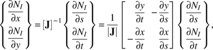
where |J| is the Jacobian and is the determinant of [J].
Since isoparametric mapping is used, the above Jacobian can be obtained by differentiating the relation in eq. (7.15) with respect to s and t. For example,

A similar expression can be obtained for ![]() and
and ![]() by replacing xi with yi. Note that
by replacing xi with yi. Note that ![]() is the function of t only, while
is the function of t only, while ![]() is the function of s only.
is the function of s only.
As seen from eq. (7.17), the derivative of the shape function cannot be obtained if the Jacobian is zero anywhere in the element. In fact, the mapping relation between (x, y) and (s, t) is not valid if the Jacobian is zero or negative anywhere in the element (–1 ≤ s, t ≤ 1).
The Jacobian plays an important role in evaluating the validity of mapping as well as the quality of the quadrilateral element. The fundamental requirement is that every point in the reference element should be mapped into the interior of the physical element, and vice versa. When an interior point in (s, t) coordinates is mapped into an exterior point in the (x, y) coordinates, the Jacobian becomes negative. If multiple points in (s, t) coordinates are mapped into a single point in (x, y) coordinates, the Jacobian becomes zero at that point. Thus, it is important to maintain the element shape so that the Jacobian is positive everywhere in the element.

Figure 7.9 Four–node quadrilateral element

Figure 7.10 Isoparametric lines of a quadrilateral element

Figure 7.11 An example of invalid mapping
In practice, maintaining a positive Jacobian is not enough because of other potential numerical problems. For example, when the Jacobian is small, that is, ![]() , calculation of stress and strain is not accurate, and the integration of the strain energy will lose its accuracy. A small value of the Jacobian occurs when the element shape is far from a rectangle. To avoid problems due to badly shaped elements, it is recommended that the inside angles in quadrilateral elements be > 15° and < 165° as illustrated in figure 7.12.
, calculation of stress and strain is not accurate, and the integration of the strain energy will lose its accuracy. A small value of the Jacobian occurs when the element shape is far from a rectangle. To avoid problems due to badly shaped elements, it is recommended that the inside angles in quadrilateral elements be > 15° and < 165° as illustrated in figure 7.12.

Figure 7.12 Recommended ranges of internal angles in a quadrilateral element
7.3.3 Interpolation of Displacements and Computation of Strains
As we explained earlier, in an isoparametric element, the same shape functions are used for mapping and for interpolating displacements. For two‐dimensional solid mechanics problems, the quadrilateral element has eight DOFs. Then the displacements within the element can be interpolated as

where the shape functions in eq. (7.14) are used for interpolation. The difference between the previously described elements in chapter 6 (CST and rectangular elements) and the isoparametric quadrilateral element is that the interpolation is done in the reference coordinates (s, t). However, the behavior of the element is similar to that of the rectangular element because both of them are based on the bilinear Lagrange interpolation.
Now, we derive the strain‐displacement relationship for the quadrilateral element. In order make the following matrix operation convenient, we first reorder the strain components into the derivatives of displacements, as

As we discussed above, the derivatives of displacements cannot be obtained directly. Instead, we use the inverse Jacobian relation so that the derivatives of displacements are written in terms of the reference coordinates. Thus, we have


Writing the two equations together, we have

The strains can now be expressed as
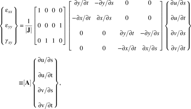
where [A] is a 3 × 4 matrix. The derivatives of the displacements with respect to s and t can be obtained by differentiating u(s,t) and v(s,t) in eq. (7.19), which involves the derivatives of the shape functions:

where the dimension of matrix [G] is 4 × 8. The strain‐displacement matrix [B] can now be written as follows:

where [B] is a 3 × 8 matrix. The explicit expression of [B] is not readily available because the matrix [A] involves the inverse of the Jacobian matrix. However, for a given reference coordinate (s, t), it can be calculated using eq. (7.20). Note that the strain‐displacement matrix [B] is not constant as in CST elements. Thus, the strains and stresses within an element vary as a function of s and t coordinates.

Figure 7.13 Mapping of a rectangular element
7.3.4 Finite Element Matrix Equation
As in the case of the CST element, the element stiffness matrix can be calculated from the strain energy of the element. By substituting for strains from eq. (7.20) into the strain energy in eq. (5.72) we have

where [k(e)] is the element stiffness matrix. Calculation of the element stiffness matrix has two challenges. First, the integration domain is a general quadrilateral shape, and second, the strain–displacement matrix [B] is written in (s, t) coordinates. Thus, the integration in eq. (7.21) is not trivial. Using the idea of mapping the physical element into the reference element, we can perform the integration in eq. (7.21) in the reference element. Since the reference element is a square and it is defined in (s, t) coordinates, the above two challenges can be resolved simultaneously. Again, the Jacobian plays an important role in transforming the integral to the reference element. Let us consider an infinitesimal area dA of the physical element that is mapped into an infinitesimal rectangle ds⋅dt in the reference element. Then, the relation between the two areas becomes
Thus, the element stiffness matrix in the reference element can be written as

Although the integration has been transformed to the reference element, still the integration in eq. (7.23) is not trivial because the integrand cannot be written down as an explicit function of s and t. Note that the matrix [B] includes the inverse of the Jacobian matrix. Thus, it is going to be extremely difficult, if not impossible, to integrate eq. (7.23) analytically. However, since the integral domain is a square, numerical integration can be used to calculate the element stiffness matrix. Numerical integration methods using Gauss quadrature, which is the most popular method, will be discussed in the following section. Similar to the other elements, the strain energy of entire solid can be obtained using eq. (6.24) in chapter 6, which involves the assembly process.
The potentials of applied loads can be obtained by following a similar procedure as the CST and rectangular elements. The potential energy of concentrated forces and distributed forces will be the same with that of the CST element. The potential energy of the body force can be calculated using eq. (6.32), except that the transformation in eq. (7.22) should be used so that the integration be performed in the reference element. For rectangular elements, the uniform body force yields the equally divided nodal forces. In the case of the quadrilateral element, however, the work–equivalent nodal forces will not divide the body force equally because the Jacobian is not constant within the element. The numerical integration can be used for integrating eq. (6.32).
Using the principle of minimum total potential energy in eq. (6.36), a similar global matrix equation for the quadrilateral elements can be obtained. Applying boundary conditions and solving the matrix equations are identical to those of the CST element. After solving for nodal displacements, strain and stress of the element can be calculated using eqs. (7.20) and (6.38), respectively.
7.4 NUMERICAL INTEGRATION
7.4.1 Gauss Quadrature
As discussed before, it is not trivial to analytically integrate the element stiffness matrix and body force for the quadrilateral element. Although there are many numerical integration methods available, Gauss quadrature is the preferred method in the finite element analysis because it requires fewer function evaluations compared to other methods. We will explain the one–dimensional Gauss quadrature first.
In Gauss quadrature, the integrand is evaluated at predefined points (called Gauss points). The sum of these integrand values, multiplied by integration weights (called Gauss weight) provides an approximation to the integral:

where n is the number of Gauss points, si are the Gauss points, wi are the Gauss weights, and f(si) is the function value at the Gauss point si. The locations of Gauss points and weights are derived in such a way that with n points, a polynomial of degree 2n–1 can be integrated exactly. Note that the integral domain is normalized, that is, [−1, 1], which is why the range of the one‐dimensional reference element in section 7.2 is defined by [−1, 1]. The Gauss quadrature performs well when the integrand is a smooth function. Table 7.2 shows the locations of the Gauss points and corresponding weights.
Table 7.2 Gauss quadrature points and weights
| NG | Integration Points (si) | Weights (wi) | Exact polynomial degree |
| 1 | 0.0 | 2.0 | 1 |
| 2 | ±0.5773502692 | 1.0 | 3 |
| 3 | ±0.7745966692 0.0 |
0.5555555556 0.8888888889 |
5 |
| 4 | ±0.8611363116 ±0.3399810436 |
0.3478546451 0.6521451549 |
7 |
| 5 | ±0.9061798459 ±0.5384693101 0.0 |
0.2369268851 0.4786286705 0.5688888889 |
9 |
Two‐dimensional Gauss integration formulas can be obtained by combining two one‐dimensional Gauss quadrature formulas as shown below:

where si and tj are Gauss points, m is the number of Gauss points in s direction, n is the number of Gauss points in the t‐direction, and wi and wj are Gauss weights. The total number of Gauss points becomes m × n. Figure 7.14 shows few commonly used integration points.

Figure 7.14 Gauss integration points in two‐dimensional parent elements
The element stiffness matrix in eq. (7.23) can be evaluated using 2 × 2 Gauss integration formulas:


Figure 7.15 Numerical integration of a square element
In general, the 2 × 2 Gauss quadrature is not exact for quadrilateral elements. The exact results in the above example occur because the element shape is a square.
7.4.2 Lower–Order Integration and Extra Zero–Energy Modes
It is important that the proper order of Gauss quadrature should be used. Otherwise, the element may show undesirable behavior. One of the well‐known phenomena of lower–order integration is extra zero energy modes. The zero‐energy mode is the deformation of an element without changing its strain energy. In plane solids, there are three types of deformations (more precisely, motions) that do not change the strain energy: x‐translation, y‐translation, and z‐rotation. Figure 7.16 illustrates these modes. Since the relative locations of nodes do not change, the stress and strain of the elements are zero, and the strain energy remains constant. In finite element analysis, these modes should be fixed by applying displacement boundary conditions. Otherwise, the stiffness matrix will be singular, and there will be no unique solution.

Figure 7.16 Three rigid‐body modes of plane solids
While the zero‐energy modes in figure 7.16 are proper modes, there are improper modes, called extra zero‐energy modes, which often occur when an element is under‐integrated. For example, if a square element is integrated using 1 × 1 Gauss quadrature, there will be two extra zero‐energy modes in addition to the three rigid‐body modes. Figure 7.17 illustrates the two extra zero‐energy modes of plane solids. It is clear that the element is being deformed, but the centroid (the quadrature point) of the element does not experience any deformation and hence the strain energy remains constant. In other words, the element will deform without having externally applied forces, which is a numerical artifact. Thus, the extra zero‐energy modes must be removed in order to obtain meaningful deformation.

Figure 7.17 Two extra zero‐energy modes of plane solids
The most common way of checking whether extra zero‐energy modes exists is by computing the eigenvalues of the stiffness matrix. For a plane solid, the number of zero eigenvalues must be equal to three, which represents the three rigid‐body motion. However, the element stiffness matrix with 1 × 1 integration will have five zero eigenvalues corresponding to five zero energy modes shown in figure 7.16 and figure 7.17. In the following example, we will show another method of checking for extra zero‐energy modes.
7.5 HIGHER‐ORDER QUADRILATERAL ELEMENTS
The quadrilateral element described in the previous section is a bilinear element that is widely used but often requires a high mesh density for the solution to converge toward the exact solution. The four‐node quadrilateral interpolates the variable linearly along the edge. Higher‐order elements can similarly be derived, which are quadratic or cubic along the edges. These elements have more nodes per element and therefore are more computationally expensive than bilinear elements. But on the other hand, one can obtain a better quality solution with fewer elements in the mesh. Since the geometry is also interpolated using the same shape functions, the geometry is also better approximated by these elements. For all isoparametric quadrilateral elements, the shape functions are expressed in terms of the parametric coordinates. Here we will look at several higher‐order quadrilateral elements.
When the order of element goes up, the element has more nodes and DOFs. Therefore, it is possible to choose the interpolation using higher‐order polynomials. The question is how to choose an appropriate order of polynomials for a given element. A useful strategy is based on the polynomial triangle, similar to Pascal’s triangle, shown in figure 7.18. In the case of three‐dimensional space, a similar polynomial pyramid can be defined. In the figure, polynomials are chosen from the top to bottom. The chosen polynomials are also called the basis. For example, the linear triangular element has three nodes, so the interpolation can choose {1, s, t}. In the case of a quadrilateral element, the first three bases are the same as a triangular element. Additional bases can be chosen from next level. Among s2, st, and t2, st is chosen because the interpolation should perform equally for both the s‐ and t‐direction.
In the polynomial triangle, it is important for the interpolation functions to include the first level, that is, 1, and the second level, s and t. The first level is required for the element to represent rigid body motion properly, while the second level is required for the constant strain field. If an interpolation scheme misses these two levels, it is possible that the element can generate fictitious strain under rigid body motion.

Figure 7.18 Polynomial triangle
7.5.1 Nine‐Node Lagrange Element
The 9‐node Lagrange element is a bi‐quadratic element whose shape functions can be derived using the Lagrangian interpolation approach and hence is a part of the family of Lagrange elements. Figure 7.19 shows the reference element in the parametric space, which is again a 2 × 2 square with its centroid at the origin. While the nodes of the physical element can be numbered arbitrarily, the element connectivity must be defined in the sequence shown in figure 7.19. Here we use a node‐numbering scheme where the first four nodes are the corners going in the counterclockwise direction. The next four nodes are the mid‐edge nodes, and finally, the last node is at the centroid of the element.

Figure 7.19 9‐node Lagrange element in parametric space
In the case of a heat conduction problem, the temperature T(s, t) is the scalar field to interpolate. In the case of solid mechanics, displacements, u(s, t) and ![]() , are the vector field to interpolate. In this case, since each node has two DOFs, uI and vI, u(s, t) and
, are the vector field to interpolate. In this case, since each node has two DOFs, uI and vI, u(s, t) and ![]() are interpolated independently. Therefore, we look for an interpolation scheme that uses nine nodal DOFs. From the polynomial triangle in figure 7.18, the first three levels include six terms, and we need additional three terms. Among s3, s2t, st2, t3, there is no way that we can maintain symmetry by choosing three out of four. Instead, we choose two terms, s2t and st2, from this level, and choose the last term from next level, s2t2. Therefore, the interpolation of a scalar field, for example, displacement u(s, t) within this element can be expressed as a polynomial in s and t in the following form:
are interpolated independently. Therefore, we look for an interpolation scheme that uses nine nodal DOFs. From the polynomial triangle in figure 7.18, the first three levels include six terms, and we need additional three terms. Among s3, s2t, st2, t3, there is no way that we can maintain symmetry by choosing three out of four. Instead, we choose two terms, s2t and st2, from this level, and choose the last term from next level, s2t2. Therefore, the interpolation of a scalar field, for example, displacement u(s, t) within this element can be expressed as a polynomial in s and t in the following form:
Using the condition that displacement at node i is ui, we could solve for the constants ai and substitute it back to express the interpolation in the standard form using shape functions.

Alternatively, we can derive the shape functions using the requirement that ![]() at node i and zero at all other nodes. In order for N1(s, t) to be zero at all other nodes, it must have the form
at node i and zero at all other nodes. In order for N1(s, t) to be zero at all other nodes, it must have the form
This ensures that N1 is zero along the lines ![]() ,
, ![]() ,
, ![]() , and
, and ![]() along which all the other nodes are located. Furthermore, we can determine k such that
along which all the other nodes are located. Furthermore, we can determine k such that ![]() . This yields
. This yields ![]() or
or ![]() . The shape functions for the other corner nodes can also be derived in a similar fashion yielding the following shape functions for the corner nodes.
. The shape functions for the other corner nodes can also be derived in a similar fashion yielding the following shape functions for the corner nodes.
The shape functions of the mid‐edge nodes such as node 5 should be zero along all the other edges as well as at the origin; therefore, it must be of the form:
Again the constant k can be derived such that N5 is unity at node 5 or ![]() and
and ![]() . Similarly, we can derive the other mid‐edge node shape functions as
. Similarly, we can derive the other mid‐edge node shape functions as
Finally, the last node, which is at the centroid of the element has a shape function that is zero along all the edges of the element and is unity at the centroid.
These shape functions are quadratic along the edges of the element, and therefore, the interpolation of the field variable will also be quadratic. For this element to be isoparametric, the mapping between the reference element and the physical element must be constructed using the same shape functions that we have derived above for interpolation. The mapping or the geometry interpolation is, therefore, bi‐quadratic, which implies that the edges of the element will be parabolic allowing this element to better approximate curved boundaries than the bilinear element. As discussed earlier for the one‐dimensional quadratic element, the placement of the nodes in the real element is critical to ensure that the mapping is uniform. The mid‐edge nodes of the real elements in the mesh must be at the midpoint of the edges and likewise, the last node must be at the centroid of the element.
7.5.2 Eight‐Node Serendipity Elements
A two‐dimensional quadratic element with just 8 nodes is possible that has only corner nodes and mid‐edge nodes as shown in figure 7.20. The first eight shape functions of the 9‐node element cannot be used here as the shape functions for this element because all those shape functions are zero at the centroid, and therefore any interpolation within the element will also be zero. We need to derive shape functions that satisfy Kronecker’s delta condition in eq. (7.1) but are not simultaneously zero at the centroid.

Figure 7.20 8‐node serendipity element in parametric space
It is easy to derive such shape functions for the mid‐edge nodes. For example, the shape function for node 5 must be zero at the edges ![]() and
and ![]() and will be of the form
and will be of the form ![]() . The constant k must equal one half for this shape function to have a unit value at the node 5. Following this procedure, the shape functions of the mid‐edge nodes can be derived as
. The constant k must equal one half for this shape function to have a unit value at the node 5. Following this procedure, the shape functions of the mid‐edge nodes can be derived as
The shape functions of the corner nodes must be zero at the opposite edges. These conditions are satisfied also by the shape functions of the 4‐node elements. However, for the 8‐node element, we want the shape functions to be zero at the midpoint of the adjacent edges as well. Figure 7.21 shows the plot of the shape function for node 1 of a 4‐node isoparametric element. At the midpoint of the adjacent edges of node 1, this shape function has a value of one half.

Figure 7.21 Shape function for node 1 of a 4‐node element
To derive shape functions for the 8‐node element, we need to reduce the value of the 4‐node element shape function to zero at node 5 and node 8. This can be accomplished using the shape functions for nodes 5 and 8 as
A similar procedure can be employed to derive the shape functions of all the corner nodes as
The 8‐node element is also quadratic along the edges of the element and therefore has parabolic edges, as the 9‐node element. Therefore it is able to represent curved boundaries with the same accuracy as the 9‐node element but with one fewer node. For this reason, the 8‐node element is the more popular quadratic element.
The technique employed here to derive the shape functions of an 8‐node element can also be used to derive shape functions for 5‐node, 6‐node, or 7‐node elements. Such elements are needed for adaptive mesh regeneration techniques where instead of increasing the number of elements, the order of the elements is increased in regions where there is a stress concentration. In order to transition from a higher‐order element, such as an 8‐node element, to a lower‐order element, such as a 4‐node element, one needs transition elements in between that have 3 nodes along their edges on one side and only 2 nodes on the opposite edge. This can be achieved by a 5‐node element. Such elements are therefore often referred to as transition elements.
7.5.3 Practical Considerations
Higher‐order elements are able to approximate the solution better than lower‐order elements and, in general, for the same number of elements, they would provide a better quality solution. Another way to compare elements is to compare the number of elements needed to reach the same level of accuracy or to obtain a converged solution. Again, the higher‐order elements are better in this regard because you can use a much lower mesh density to reach the same level of accuracy. However, higher order elements have more nodes per element, and they also require higher‐order Gauss quadrature for accurate integration when computing the stiffness matrix. Therefore, from the viewpoint of the cost of computation, higher‐order elements can be more expensive because the cost of computation to obtain a converged result is often higher even though the number of elements in the mesh is lower.
The elements discussed in this chapter interpolate the field variables such that it is continuous between elements so that the interpolation is said to satisfy C0 continuity. But the derivatives of these variables are not guaranteed to be continuous or in other words, the interpolation does not satisfy C1 continuity across boundaries. This implies that quantities such as stress /strain and heat flux are not continuous between elements. The field variables such as displacement (or temperature) also converge faster with increasing mesh density than derived quantities like stress/strain (or heat flux). If the stress is computed at a node or edge, the value obtained will be different for each element adjacent to that node. To plot such quantities, finite element analysis software programs smooth the results. One simple approach to smooth the solution is to compute the stresses at a node for each adjacent element and then to use the average value as the nodal value, which can be interpolated to obtain a continuous solution. The results for stresses and other similar derived quantities are most accurate at the integration (Gauss) points. Therefore, average nodal values are often computed by extrapolating from the nearest integration points. Another popular approach involves fitting a patch (curve for two‐dimension and surface for three‐dimension) that best approximates the values at the nearest integration point to estimate the value at the node.
If the structure being analyzed has stress concentration or the solution has large gradients, then smaller elements are needed in such regions. In regions where the solution is nearly constant and the gradients are small, larger elements would suffice, so it is not beneficial to globally reduce the size of the elements. To reduce computation, the mesh must be locally refined in regions that need smaller‐sized elements. Adaptive mesh refinement capability is available in most commercial software to automatically refine the initial uniform mesh in regions where the solution has large errors. This can be achieved by sub‐dividing the elements in such regions to create smaller‐sized elements. This method is referred to as h‐adaptive mesh refinement. This technique is used in an example later in this chapter to show why such refinement is necessary to compute stresses accurately at stress concentrations.
Another approach for adaptive mesh refinement is p‐adaptive mesh refinement where the order of the elements is raised in regions where the solution is not accurate. This is illustrated in figure 7.22 where the left‐most element has been converted to an 8‐node quadratic element to improve accuracy. In order to do so, it is necessary to have transition elements like the 5‐node element shown in the figure because 4‐node elements and 8‐node elements are not compatible and cannot be next to each other. Along the edges, displacement is interpolated linearly for 4‐node elements while it is interpolated as a quadratic for an 8‐node element. This means that if these two types of elements are side by side, then along the shared edge, the displacement will not be continuous.
Figure 7.22 5‐node transition element
The 5‐node element shown in figure 7.22 is a transition element that uses quadratic interpolation along the edge that it shares with the 8‐node element, and these two elements share the 3 nodes along this edge. Along the opposite edge where it is adjacent to the 4‐node element it has linear interpolation and only two nodes. Shape functions for such an element can be derived using the same technique that we used earlier for the 8‐node serendipity element. Other types of transition elements may be needed in a mesh during p‐adaptive refinement such as elements with 6 nodes and 7 nodes depending on the type of element it is adjacent to at each edge.
7.6 ISOPARAMETRIC TRIANGULAR ELEMENTS
7.6.1 Collapsed 4‐Node Quadrilateral Element
In the previous chapters, we have seen the classical triangular element, which is not formulated as an isoparametric element. Since we explained the benefits of isoparametric elements, it would be good to derive the isoparametric formulation for a triangular element. There are a couple of ways to derive the isoparametric triangular element. First, the 4‐node quadrilateral isoparametric element in section 7.3 can be converted to a triangular element by collapsing or merging two of its nodes together into one node. By doing so, we get a mapping relation between a square in the parametric space to a triangle in the physical coordinates. This is illustrated in figure 7.23 where nodes 3 and 4 are merged and mapped to the same physical node.

Figure 7.23 Triangular element by collapsing a 4‐node quadrilateral
In practice, this can be easily achieved by creating a connectivity table for the element in which two of the nodes are identical. This implies that if only the 4‐node isoparametric element is available in a finite element analysis software program, then one can still use a mesh that contains triangular elements. This also facilitates the use a mesh that contains both quadrilateral and triangular elements. For the examples shown in figure 7.23, the row in the connectivity table corresponding to this element will look as follows:
| Element # | 1 | 2 | 3 | 4 |
| 45 | 51 | 57 | 61 | 61 |
The interpolation of a scalar field u(s, t) in parametric space for the 4‐node element is simplified to obtain the three shape functions of the collapsed element where we assume that two of the nodes are the same.
The three shape functions of the triangular element thus obtained are
The mapping can also be now expressed using these three shape functions for the collapsed 4‐node element. This provides a mapping from the square in parametric space to a triangle in real space.

It is interesting to note that this element is similar to the classical triangular elements in terms of the quality of the interpolation within the element. Since it interpolates between three nodal values, we expect that the interpolation in the real space is linear because three points define a plane. Therefore we also expect that the derivatives should be constant. The following example illustrates this idea and explores some numerical aspects.

Figure 7.24 Triangular element in physical space
7.6.2 Three‐Node Linear Triangular Element
Another way of formulating the isoparametric triangular element is to use a mapping where the reference element is assumed to be a right triangle that is mapped to an arbitrary triangle in the physical space as shown in figure 7.25. This approach has the same advantages as the quadrilateral isoparametric elements. The shape functions are derived with respect to the parametric coordinates to perform interpolation and are therefore very simple functions. The stiffness matrix can be computed by integrating over a right triangle of fixed size and shape in the parametric space.

Figure 7.25 3‐node isoparametric triangular element
The shape functions for a 3‐node linear element can be expressed simply as:
The shape functions for this element are identical to the coordinates in the parametric space. The third shape function can also be thought of as a coordinate, even though only any two of (r, s, t) are sufficient to identify the location of a point in the triangle. Note that the third coordinate t is unity at node 3 and is zero along the line between nodes 1 and 2. This three‐node element is identical in behavior to the classic 3‐node triangle discussed earlier in terms of the quality of the results obtained. Therefore, when used for two‐dimensional solid mechanics, this element is a constant‐strain triangle. As strain is approximated as constant within each element, these elements are not very accurate and must be used only to obtain rough, qualitative results for displacement. Stresses and strains computed using this element are likely to be inaccurate unless the mesh is very dense. Despite these shortcomings, these elements are popular and available in most commercial software since these elements are computationally very inexpensive and often the user may only need a qualitative answer, for example, to visualize the deformation pattern. Mesh generation is also easier for triangular elements and automated mesh generation is available for triangular elements in many commercial finite element analysis software programs.
7.6.3 Six‐Node Quadratic Element
As we saw earlier for the isoparametric quadrilateral elements, it is fairly easy to derive the shape functions of the higher‐order triangular elements using the Kronecker’s delta conditions. Consider a 6‐node quadratic element with 3 corner nodes and 3 mid‐edge nodes as shown in figure 7.26. In the parametric coordinates, we will assume that the six nodes are located at: (1, 0), (0, 1), (0, 0), (0.5, 0.5), (0, 0.5) and (0.5, 0) and numbered in that order.

Figure 7.26 Six‐node isoparametric triangular element
For node 1, we want the shape function to be zero along the lines ![]() and
and ![]() and equal to unity at (1, 0). Similarly, N4 should be zero at
and equal to unity at (1, 0). Similarly, N4 should be zero at ![]() and
and ![]() and have a unit value at (0.5, 0.5). Using such conditions, the shape functions for this element can be derived as:
and have a unit value at (0.5, 0.5). Using such conditions, the shape functions for this element can be derived as:

In the preceding equations, ![]() , and it can be easily verified that these shape functions satisfy the Kronecker’s delta condition. The interpolation of the field variables for these triangular elements is done the same way as all other isoparametric elements yielding an interpolation in the parametric coordinate system.
, and it can be easily verified that these shape functions satisfy the Kronecker’s delta condition. The interpolation of the field variables for these triangular elements is done the same way as all other isoparametric elements yielding an interpolation in the parametric coordinate system.

The mapping between parametric and real space is again constructed using the shape functions so that the edges of a linear element are straight lines while the edges of a quadratic element are parabolic.

7.6.4 Numerical Integration for Isoparametric Triangular Elements
As in the case of quadrilateral isoparametric elements (see section 7.4), Gauss quadrature is used for integrating over isoparametric triangular elements as well. Again, the integral is evaluated as the sum of the values of the integrand at Gauss points multiplied by Gauss weighting values:

where n is the number of Gauss points, (ri, si) are the Gauss points, wi are the Gauss weights, and f(ri, si) the function value at the Gauss points. A polynomial of degree 2n–1 can be integrated exactly using n‐point integration. The domain of the integral is normalized to [−1, 1] for convenience. Even if the integrand is not a polynomial, Gauss quadrature performs well when the integrand is a smooth function that can be well‐approximated by a polynomial. Table 7.3 shows the locations of the Gauss points and the corresponding weights for quadrature over triangles.
Table 7.3 Gauss quadrature points and weights for triangles
| Integration Points | Weights | ||
| n | ri | si | wi |
| 1 | 1/3 | 1/3 | 1.0 |
| 3 | 1/6 1/6 2/3 |
2/3 1/6 1/6 |
1/6 1/6 1/6 |
| 4 | 1/3 1/5 1/5 3/5 |
1/3 1/5 3/5 1/5 |
−9/32 25/96 25/96 25/96 |
| 6 | 0.445948490915965 0.445948490915965 0.108103018168070 0.091576213509771 0.091576213509771 0.816847572980458 |
0.445948490915965 0.108103018168070 0.445948490915965 0.091576213509771 0.816847572980458 0.091576213509771 |
0.111690794839005 0.111690794839005 0.111690794839005 0.054975871827661 0.054975871827661 0.054975871827661 |
7.7 THREE‐DIMENSIONAL ISOPARAMETRIC ELEMENTS
Three‐dimensional finite elements are rather straightforward extensions of similar two‐dimensional elements, and no new concepts or methodology is needed. In general, three‐dimensional elements are far more computationally expensive than two‐dimensional elements not only due to the larger number of nodes and equations but also because numerical integration is more expensive in three dimensions. So if it is possible to model a structure as two‐dimensional, then it is better to avoid three‐dimensional models. Using simplified models that use half or a quarter of the structure, if the symmetry of the structure allows it, can also help to reduce the cost of computation. Popular elements in three dimensions are tetrahedral and hexahedral elements even though specialized elements shaped like pyramids or wedges are also available in some software packages. Below we present the shape functions of a few isoparametric elements that are commonly found in finite element software.
7.7.1 Four‐Node Tetrahedral Element
The 4‐node tetrahedral element is similar to the 3‐node triangular element. The shape functions and the displacement interpolation are linear while the strain components are constant within the element. The shape of the element in parametric coordinates and the mapping to the real space are shown in figure 7.27. For this mapping, the shape functions are identical to the parametric coordinates.


Figure 7.27 Four‐node isoparametric tetrahedral element
For this element, the interpolation of the variable is linear within the element. For a field variable such as temperature, the interpolation for the three‐dimensional element is no different than for two‐dimensional elements.

As the shape functions are linear, the physical quantities that are proportional to the gradient of the field variable such as strains, stresses, or heat flux are constant within the element. Therefore, the quality of the solution is not likely to be very good using this element especially when the strain is varying rapidly, for example, near regions with stress concentration. This element should be used with caution, and it is important to be aware that the solution can have large errors in stress/strain when mesh density is inadequate. As with the other parametric elements, the mapping from the parametric to the real space is accomplished using shape functions as

As with the 3‐node triangular element, the 4‐node tetrahedron has constant strain within the element and is, therefore, a constant strain tetrahedron (CST). Tetrahedral elements are popular in finite element analysis software due to the ease of mesh generation compared to hexahedral elements. Automated mesh generation is available in many finite element analysis programs for tetrahedral elements. But the 4‐node element is not very accurate, so the 10‐node quadratic tetrahedral element should be used when more accurate results are needed especially for stresses or heat flux.
7.7.2 10‐Node (Quadratic) Tetrahedral Element
The quadratic tetrahedral element is shown in figure 7.28. As shown in the figure, it has nodes at the midpoint of all the edges in addition to the nodes at the vertices. The shape functions for this element can be defined using the shape functions of the 4‐node tetrahedral element: ![]() .
.

Figure 7.28 Ten‐node isoparametric tetrahedral element
As in the previous elements, the shape functions can be derived easily using the Kronecker’s delta properties. For example, the shape function for node 1 is zero along the planes ![]() and
and ![]() , and it is unity at node 1. The shape functions are:
, and it is unity at node 1. The shape functions are:

The interpolation of field variables for this element will yield a quadratic function within the element. Therefore, we expect the gradients and quantities related to gradients such as strains and stresses to be linearly varying within the element. The shape of the element in the parametric space is its ideal shape, and any distortion of this shape in the physical space will reduce the accuracy of the numerical integration.
7.7.3 Eight‐Node Hexahedral (Brick Element)
The 8‐node hexahedral element is the three‐dimensional analog of the two‐dimensional 4‐node quadrilateral element. The hexahedral elements are often referred to as brick elements. This 8‐node element has shape functions that are trilinear, that is, linear along its edges but not internally. All eight shape functions of this element can be expressed using the following equation in index notation for ![]() .
.
In the preceding equations (ri, si, ti) are the parametric coordinates of the nodes of the elements. As shown in figure 7.29, in the parametric coordinates (r, s, t) the element is a cube of size ![]() with its centroid at the origin while in the real space it is a hexahedron where the opposite faces and edges are not necessarily parallel to each other. For the element numbering shown in the parametric space, the coordinate of node‐1 in parametric space is (−1, −1, −1) and the coordinates of the diagonally opposite node‐7 are (1,1,1).
with its centroid at the origin while in the real space it is a hexahedron where the opposite faces and edges are not necessarily parallel to each other. For the element numbering shown in the parametric space, the coordinate of node‐1 in parametric space is (−1, −1, −1) and the coordinates of the diagonally opposite node‐7 are (1,1,1).

Figure 7.29 Eight‐node isoparametric hexahedral element
The interpolation of the field variables for all the 3D elements described in this section is similar to other isoparametric elements yielding an interpolation in the r‐s‐t coordinate system. For solid mechanics, the three components of the displacement field are interpolated in the parametric space as:

Here again, the summation is over the number of nodes per element (ne). The mapping between parametric and real space is again constructed using the shape functions so that the edges of a linear element are straight lines while the edges of a quadratic element are parabolic.

The 8‐node hexahedral element is superior to the 4‐node tetrahedral element due to the fact that strains are not constant within this element, and therefore better‐quality results are obtained. However, automated mesh generation is more difficult for hexahedral elements. Earlier we discussed how a triangular element can be created by collapsing two nodes of a 4‐node quadrilateral element. Similarly, it is possible to create a pyramid element by collapsing the four nodes on any face of an 8‐node hexahedron into a single node. A wedge‐shaped element can be created by collapsing the two nodes on the opposite edges of a face.
Higher‐order hexahedral elements can be derived using the same techniques that we discussed earlier for quadrilateral elements. Popular elements include 20‐node serendipity element and 27‐node tri‐quadratic elements analogous to the 8‐node serendipity and 9‐node bi‐quadratic elements that we discussed for two dimensions. For such elements, it is important that the mesh generator places the nodes on the edges of the element at the midpoint of the edge to avoid distorting the mapping of the element from parametric to real space. For all isoparametric elements, the order of the nodes in the connectivity table should also match the order in which the nodes are numbered in parametric space.
Mesh generation is more difficult for hexahedral elements because fully automated mesh generators are rarely available. Traditional mesh generation programs require the user to subdivide the shape into simpler shapes and specify the number of nodes along the edges of the sub‐divided regions. The quality of the solution deteriorates if the element has to be severely distorted to fit the geometry. Adaptive mesh refinement is also more difficult to implement for hexahedral elements. For these reasons, tetrahedral elements are still more popular than hexahedral elements for three‐dimensional analysis.
7.7.4 Numerical Integration in Three‐Dimensional Hexahedral Elements
For three‐dimensional elements, we need to extend Gauss quadrature to three dimensions, which involves combining three one‐dimensional Gauss quadrature formulas as shown below:

where ri, sj, and tk are Gauss points, l is the number of Gauss points in the r direction, m is the number of Gauss points in s direction, and n is the number of Gauss points in the t direction, and wi, wj, and wk are the Gauss weights. The total number of Gauss points is therefore l × m × n.
The element stiffness matrix for an 8‐node hexahedral element can be evaluated using the 2 × 2 × 2 Gauss quadrature formula:

The Jacobian matrix for 3D elements is defined as:

As in the case of 2D problems, the determinant of the Jacobian is the ratio of the volumes in real space and parametric space. The Jacobian matrix is, in general, a function of the coordinates and is not constant within the element. However, if the element is regular shaped (cubes or cuboid) and the element edges are aligned with the coordinate system, then this matrix will be constant and diagonal. The numerical integration is exact only if the integrand is a polynomial. If the element is distorted and the Jacobian is not constant, then the integrand is not a polynomial because the inverse of the Jacobian will be a rational function (a ratio of polynomials). The more distorted the element is, the less accurate the numerical integration is. This is the reason why the quality of the mesh is very important to ensure the accuracy of the results. Ideally, the elements should be as close to cuboids as possible for a three‐dimensional hexahedral mesh.
7.8 FINITE ELEMENT MODELING PRACTICE FOR ISOPARAMETRIC ELEMENTS
In this section, we consider several examples where we explore some of the practical applications of the elements discussed in this chapter to model solids and structures. Many commonly used practices for selecting the right model and boundary conditions, as well as method for simplifying the model, are discussed.
7.8.1 U‐Shaped Beam
The U‐shaped aluminum frame shown in figure 7.30 has a 20 × 20 mm2 square cross section. A load P equal to a magnitude of 5 kN is located at a distance of 40 mm from the center of curvature of the curved portion of the frame. The inner radius of the curved beam is 30 mm. The Young’s modulus of the material is 69 GPa, and Poisson’s ratio is 0.33. Describe the model you would use for this structure. Compute the deflection due to the applied load and the maximum/minimum stresses in the structure.

Figure 7.30 U‐shaped beam
The structure has a uniform thickness in the z‐direction and the loads are in the x‐y plane, so clearly, this structure can be modeled using 2D elements as a plane stress problem. The structure and the loads are symmetric about the mid‐plane of the structure, so a plane stress model of half the structure can be used as shown in figure 7.31.

Figure 7.31 Plane stress model of U‐shaped beam
The load is applied as a shear stress (traction parallel to the face) at the tip of the structure, and a sliding boundary condition is used along the symmetry face. The sliding boundary condition is necessary to allow the width to change due to Poisson’s effect. In this model, sliding implies that the nodes on the edge are fixed in the vertical direction and free in the horizontal direction. In addition to this sliding boundary condition, we need some constraint to prevent rigid body motion in the horizontal direction. This can be achieved by fixing a point along the symmetry plane. In this model, we have fixed the vertex at the right end of the sliding edge.
Figure 7.32 Deflection and stress distribution in U‐shaped beam
Figure 7.32 shows the deflection and von Mises stress distribution in the structure. As expected, the maximum deflection is at the tip where the load is applied, and the maximum stress is at the symmetry plane where the vertical displacement is constrained. The stress varies through the thickness of the beam, so it is important to have sufficient elements through the thickness to capture this stress distribution accurately.
7.8.2 Plate with Holes
A steel plate with holes as shown in figure 7.33 serves as a bracket and is bolted at the top two holes and supports a load via a pin that goes through the lower hole. The dimensions of the plate are as shown in figure 7.33, and its material properties are Young’s modulus = 200 GPa and Poisson’s ratio = 0.3. The vertical load applied through the pin is 5000 N. Compute the maximum deflection and peak stress in the structure due to this applied load. What would be the appropriate model if the load were normal to the plate at the pin?
Figure 7.33 Plate with holes
The plate geometry and the applied loads are symmetric; therefore, half of this structure can be modeled as a plane stress problem. The two bolted holes can be treated as complete fixed if it is in fact very tightly bolted so that the plate is not likely to rotate about the bolts during its deformation when the load is applied. On the other hand, if it is likely to rotate, then they need to be modeled as hinges. In some finite element analysis software programs, the fixed hinge is a predefined boundary condition that can be applied to cylindrical surfaces. This is equivalent to using a cylindrical coordinate system with its origin and z‐axis along the axis of the cylindrical hole and then fixing the radial and axial components of displacement with respect to this coordinate system while allowing tangential displacement that causes rotation about the z‐axis. In this example, we will study both options to see how it affects the solution.

Figure 7.34 Pressure distribution p(ϕ) for bearing load
The load that is applied to the plate is clearly not going to be uniformly distributed along the surface of the hole. The pin will transmit the load through contact over the lower half of the hole only since it cannot pull on the upper half and furthermore the contact pressure distribution is not uniform over this region. The contact load distribution is often assumed to be parabolic, and some commercial finite element analysis software programs provide a “bearing load” option that will automatically apply this type of load distribution on cylindrical holes in the specified direction. Figure 7.34 shows the pressure distribution typically assumed for the bearing load over the lower half of the hole that supports the pin. In this example, we will explore how much the deformation of the plate would differ if the load is applied as a bearing load versus applying it as a uniform traction along the entire cylindrical surface.
Figure 7.35 shows the finite element model that can be used for this analysis where one half of the symmetric plate is modeled. Along the symmetry plane, the sliding boundary condition is applied so that the nodes are able to slide in the vertical direction while being fixed in the horizontal or x‐direction. As discussed above, the bolted hole was modeled both as fixed and later as hinged to compare the resulting deflection of the plate. Similarly, the load was applied both as uniformly distributed traction and as the parabolic bearing load in the vertical direction for comparison. As we are modeling one half of the plate, a load of 2500 N is applied, which is half the total load on the plate.

Figure 7.35 Finite element model of plate with holes
Figure 7.36(a) and (b) shows the plot of the deflection of the plate for uniform and bearing loads respectively. In both cases, the bolt hole is allowed to rotate about its axis. The von Mises stress distributions for these two models are shown in figure 7.37.

Figure 7.36 Deflection (mm) due to uniform load versus bearing load

Figure 7.37 von Mises stress (N/m2) due to uniform load versus bearing load
As can be seen in these figures, the results are significantly different when the load is applied differently even though the total magnitude of the applied load is the same. There is more deflection at the hole where the load is applied. The location where the highest stress occurs is also different. The highest stress is mostly localized near the load‐application hole when the bearing load is applied whereas it is highest near the bolted hole when the load is applied as uniformly distributed.
The results are summarized in table 7.4 where the maximum displacement and the maximum von Mises stresses are listed for the various options for boundary conditions and load application. As discussed earlier, there is a significant difference in displacement and stresses for different load distributions, but the results do not differ much between fixing the bolt hole versus allowing it to rotate. As expected, we get a slightly larger maximum displacement when the bolt hole is allowed to rotate compared to when it is fixed.
Table 7.4 Results for the plate with holes
| Result | Uniform load and Rotating at bolt |
Bearing load and Rotating at bolt | Bearing load and Fixed at bolt |
| Max. Displacement (mm) | 4.323 × 10⁻³ | 9.479 × 10⁻³ | 9.277 × 10⁻³ |
| Max. Stress (Von‐Mises, MPa) | 19.12 | 56.40 | 56.49 |
If the load were normal to the plate, then it can no longer be modeled as a two‐dimensional plane stress problem. The geometry alone does not determine the type of model that is needed. Obviously, the applied load plays an important role since the deformation due to this load will now be normal to the plate and no longer in the plane of the plate. In this case, this plate could be modeled using a three‐dimensional finite element model as shown in figure 7.38 where the load is applied as a shear force along the surface of the hole assuming that the pin is press fitted or has a flange to transmit the load.

Figure 7.38 Plate with normal forces
As the plate bends, the stresses vary linearly through the thickness of the plate (as in a beam), and therefore several elements are needed through the thickness. In this case, ideally quadratic tetrahedrons or even higher‐order elements must be used to ensure accurate results. If this plate were very thin, as in a sheet metal where thickness may be several orders of magnitude smaller than the overall dimensions, then it becomes impractical to use three‐dimensional elements. In that case, one should use plate or shell elements that are based on plate/shell theory. These elements are beyond the scope of this text book.
7.8.3 The 3D Bracket
An alloy steel L‐shaped bracket, as shown in figure 7.39, is bolted to a rigid wall through the holes on its upright side. A stepped shaft going through the 140‐mm hole rests on this bracket and applies a 10,000‐N vertical load on the bracket. Assume that the load is transmitted through an annular region around the hole that has a radial width of 10 mm. Compute the maximum stress due to this load assuming that the material properties are as follows: ![]() Pa and
Pa and ![]() .
.
Figure 7.39 A 3D bracket drawing
The geometry of this bracket is non‐planar, and therefore a 2D model is obviously not applicable for this example. We will assume that the bolt joints rigidly fix the holes, and since it is against a rigid wall, we will fix the back side of the bracket as well. The geometry and the loads are symmetric, so one could create a model using half the geometry, but the whole geometry is modeled here for better visualization of the results. To apply the load, the face supporting the load is split to create an annular region as shown in figure 7.40. Most CAD software programs provide the capability to split a face by sketching a region on it. The mesh generator then automatically creates a mesh that includes the edges of the faces as shown in the mesh in figure 7.41(a). This allows a normal pressure to be applied on the face.

Figure 7.40 A 3D bracket loads and boundary conditions
The initial mesh and the computed von Mises stresses are shown in figure 7.41(a) and (c), respectively. There is a stress concentration at the rounded edge, which is not accurately calculated by this default mesh. Increasing the mesh density will cause the computed stress at this corner to increase. One way to increase the mesh density is to specify a smaller element size, but doing so for the entire mesh is inefficient. Therefore, most FEA programs provide various methods to locally refine the mesh where needed. For example, a smaller element size can be specified on the rounded face at the corner so that the mesh generator will create a mesh where the element size is small near the corner and gradually increases to the default size away from this rounded corner. Alternatively, one could use adaptive mesh generation schemes where the software automatically determines regions with high error and refines the mesh only in these regions. The error can be estimated in several ways such as checking how well the solution satisfies the equilibrium equations or by the magnitude of the discontinuity in the derivatives of the displacement between elements. As stated earlier, there are two approaches that are popular for adaptive refinement: p‐adaptive and h‐adaptive. In the p‐adaptive refinement, the order of the elements is raised in regions with high error. Here we will use h‐adaptive refinement, where the elements are sub‐divided into smaller elements in regions where the error is high. Figure 7.41(b) and (d) shows the locally refined mesh obtained by h‐adaptive refinement and the corresponding computed von Mises stress distribution, respectively. The refined mesh is able to more accurately determine the stress at the rounded edge, and the computed stresses are therefore much higher than those computed with the default mesh. Notice that the elements at the round are extremely small, and it would not be efficient or practical to use such small elements through the entire structure. The h‐adaptive refinement determines that the solution is not accurate at the corner with the initial mesh and automatically subdivides the elements in this region until the desired accuracy is achieved.

Figure 7.41 h‐adaptive mesh refinement for 3D bracket
7.9 PROJECTS
7.10 EXERCISES
- Answer the following descriptive questions.
- Explain what the “isoparametric” mapping means.
- For a 1D 3‐node quadratic element, what is the condition to make the Jacobian constant?
- When quadratic elements are used, will displacements be continutous across the element boundary with the adjacent element? Will strains be continuous?
- The stress in a bar varies linearly. When three nodes are equally spaced in the bar, which result is more accurate, two linear elements or one quadratic element?
- What will happen if the shape of an element is distorted in a such a way that there is a concave region within the element?
- List possible problems when the Jacobian of an element is negative.
- How many Gauss quadrature points are required to accurately integrate a polynomial of order 7?
- How many zero eigenvalues are expected for the properly integrated stiffness matrix of a quadrilateral element?
- When the stiffness matrix of a quadrilateral element has four zero eigenvalues, explain the possible cause of the problem.
- Explain why it is not acceptable to put a 4‐node quadrilateral element adjacent to an 8‐node quadrilateral element in a finite element mesh.
- Why is numerical quadrature needed for 2D and 3D elements?
- What are the main sources of error in the solutions obtained using isoparametric elements?
- The nodal coordinates and corresponding displacements in a plane triangular element shown in the figure are given in the table below. Use isoparametric formulation where
 ,
,  , and
, and 
Node number (x,y) (mm) u (mm) v (mm) 1 (3,0) 1 1 2 (0,3) 2 0 3 (0,0) 0 0 - What is the parametric coordinates of the point P whose real coordinates are (x,y) = (1,1)?
- Calculate the displacement vector at this point.
- Calculate the strain at this point.

- The quadrilateral element shown in the figure has the nodal displacement of {u1, v1, u2, v2, u3, v3, u4, v4} = {–1, 0, –1, 0, 0, 1, 0, 1}.
- Find the (s, t) reference coordinates of point A (0.5, 0) using the isoparametric mapping method.
- Calculate the displacement at point B whose reference coordinate is (s,t) = (0,–0.5)
- Calculate the Jacobian matrix [J] at point B.

- A four–node quadrilateral element is defined as shown in the figure.
- Find the coordinates in the reference element corresponding to (x, y) = (0, 0.5).
- Calculate the Jacobian matrix as a function of s and t.
- Is the mapping valid? Explain your answer.

- Consider the isoparametric quadrilateral element shown in figure 7.9(a).
- Calculate the (s,t) coordinates of the point (x,y) = (1.3,0.6), which lies on the 2‐3 edge.
- Given that the displacements at all the nodes are zero except v3 = 0.02 at node 3, calculate the value of v at the point (x,y) = (1.3,0.6).
- For the rectangular element shown determine the strain εxx at the centroid of the element using the isoparametric formulation. The nodal coordinates in the figure are in meters. The nodal displacements given in the table are also in meters.
Node Number 1 2 3 4 u (m) 0 1 2 0 v (m) 0 1 2 0 
- For the 4‐node plane strain finite element, finite element computation yields the displacements at the nodes as follows: {u1, v1, u2, v2, u3, v3, u4, v4} = {–1, 0, –1, 0, 0, 1, 0, 1} × 10−4. The connectivity table is as shown in the table.
The local and global node numbering are shown in the physical and parametric spaces, respectively, in the figure above.Element Local node 1 Local node 2 Local node 3 Local node 4 i 5 7 16 14 - Where is the point (s, t) = (0.0, 0.0), located in the global (x, y) coordinates?
- Determine the Jacobian matrix for this element.
- Find the derivate of u with respect to x and y, (
 ,
,  ) at the centroid.

- A quadrilateral element in the figure is mapped into the parent element.
- A point P has a coordinate (x, y) = (½, y) in the physical element and (s, t) = (−½, t) in the parent element. Find the y and t coordinates of the point using isoparametric mapping.
- Calculate the Jacobian matrix at the center of the element.
- Is the mapping valid? Explain your answer.

- Consider the plane stress 4–node element shown in the figure. Its global node numbers are shown in the figure with the element connectivity in the table. The coordinates of the nodes in the global x‐y coordinate system is shown next to each node. Nodal displacements are given as {q}T = {u51, v51, u52, v52, u63, v63, u64, v64} = {0, 0, 0.1, 0, 0.1, 0.1, 0, 0}.
- Determine the displacement at the point (x, y) = (0.75, 0.75) by interpolating the nodal displacements.
- Compute the Jacobian matrix at the point in (a).
- Compute strain εyy at the centroid of the element.

Element # Local node 1 Local node 2 Local node 3 Local node 4 27 51 52 63 64 - A linearly varying pressure p is applied along the edge of the 4–node element shown in the figure. The finite element method converts the distributed force into an equivalent set of nodal forces {Fe} such thatwhere T is the applied traction (force per unit area), and u is the vector of displacements. Since the applied pressure is normal to the surface (in the x‐direction), the traction can be expressed as T = {p, 0}T, where p can be expressed as p = p0(t + 1)/2, where t = −1 at node 1 and t = +1 at node 4. The length of the edge is L. Integrate the left‐hand side of the above equation to compute the work–equivalent nodal forces {F(e)} when {q(e)}T = {u1, v1, u2, v2, u3, v3, u4, v4}.


- Determine the Jacobian matrix for the following isoparametric elements. If the temperatures at the nodes of both above elements are {T1, T2, T3, T4} = {100, 90, 80, 90}, compute the temperature at the midpoint of the element and at the mid point of the edge between connecting nodes 1 and 4.

- Integrate the following function using one‐point and two‐point numerical integration (Gauss quadrature). The exact integral is equal to 2. Compare the accuracy of the numerical integration with the exact solution.

- Use 1 × 2 Gauss rule to evaluate the integral
 over the rectangular region shown in the figure. Explain why the above estimate is or is not exact.
- A six‐node finite element as shown in the figure is used for approximating the beam problem.
- Write the expressions of displacements u(x,y) and v(x,y) in terms of polynomials with unknown coefficients. For example,
 .
. - Can this element represent the pure bending problem accurately? Explain your answer. A bending moment M is applied to the edge 2–3.
- Can this element represent a uniformly distributed load problem accurately? The distributed load q is applied along the edge 4–6–3.

- Write the expressions of displacements u(x,y) and v(x,y) in terms of polynomials with unknown coefficients. For example,
- Consider a quadrilateral element shown in the figure below. The nodal temperatures of the element are given as {T1, T2, T3, T4} = {80, 40, 40, 80}.
- Compute the expression of the temperature T along the line ξ that connects nodes 3 and 1. For example,
 . You can assume that ξ = 0 at node 3 and ξ = 1 at node 1. Plot the graph of T(ξ) with respect to ξ.
 - Compute the temperature gradient
 at the center of the element.

- Compute the expression of the temperature T along the line ξ that connects nodes 3 and 1. For example,
- Compute the work (or energy) equivalent nodal forces that correspond to the uniformly distributed load of Ty = 20 kN/m assuming that the element is a 9‐node quadrilateral plane strain element. Use Gauss quadrature for the integration.

- The figure below shows a 4‐node quadrilateral element in parametric space and in real space where two of the nodes are collapsed or merged to form a triangle.
- Determine the mapping functions x(s,t) and y(s,t).
- The displacement at the nodes of the element are found to be: {u1, v1, u2, v2, u3, v3} = {1, 0, 0, 2, 0, 0}x10−3in. Compute the displacement field u(s,t) and v(s,t).
- Compute the Jacobian matrix.
- Compute the strain in the element. Is this is a constant strain element?

- An 8‐node element is shown in the figure in the parametric space.
- Derive the shape functions for this element.
- If in the real (x,y) space, an element of this type is square and has side length of 5 m, write the Jacobian matrix for this element. Assume that the edges of the element are parallel or perpendicular to the x‐ and y‐axis and that the mid‐edge nodes are at the midpoint of the edge. Hint: You do not need the shape functions.
- What is the order of Gauss quadrature that is appropriate to evaluate the stiffness matrix of this element? Will this integration be exact for the element described in (b) using this order of quadrature. Explain.
