
Chapter 8
Finite Element Analysis for Dynamic Problems
8.1 INTRODUCTION
In the previous chapters, we have discussed the static analysis of solids and structures, in which the loads are assumed to be applied slowly such that the structure is in equilibrium at every instant until the full load is applied. When the effect of velocity and acceleration can be ignored due to slow application of loads, it is called a quasi‐static loading. The structure may be considered to be under quasi‐static deformation when the inertial forces are orders of magnitude smaller than the internal forces caused by the deformation. The structure gradually deforms to produce internal forces (i.e., stresses) so that the internal forces are in equilibrium with the externally applied load. In structural mechanics, this is called static equilibrium. We did not consider the time involved, that is, how quickly the load is applied or how quickly the structure reaches equilibrium with the applied loads. However, when the loads vary rapidly with time, the inertial effects cannot be neglected. In such cases, the quasi‐static assumption is not valid and we need to compute the dynamic equilibrium, which is the main topic of this chapter. Dynamic problems are concerned with the study of motion of structures under external loads. When the external loads are time varying, or steady but applied suddenly, it will trigger dynamic effects that cause structural vibration immediately upon the application of the load. If the load is steady, then due to the presence of intrinsic damping in most materials, these vibrations will eventually die down and the structure will settle at the equilibrium position where the displacements and stresses are as calculated in static analysis. However, before reaching this equilibrium, the maximum displacements and stresses during the vibration can be significantly higher than the corresponding static values and could cause catastrophic failure.
Dynamic problems can be classified into three broader groups: Natural vibration, forced vibration, and wave propagation. The natural vibration of a structure is characterized by its natural frequencies and mode shape of vibration. These natural modes of vibration characterize the dynamic behavior of a structure and are of great value in dynamic analysis. Some forced vibration analysis techniques use the natural modes and frequencies to compute the forced response of the system. Forced vibration problems can be further divided into impact loading problems and periodic loading problems. When intense loads are suddenly applied for a short period, as in an impact problem, the response during a short initial period immediately after the impact is of importance. Whereas, when a structure is subjected to periodically fluctuating loads, we are interested in the steady‐state response which is the steady periodic response of the structure after the transient effects have dissipated due to damping. Different analysis procedures are needed for these two cases in order to make the computation efficient.
Among many different dynamic problems, we will focus on problems where the overall dynamic response of a structure is sought rather than a relatively local response, such as shock propagation. That is, we are interested in inertial problems, where wave effects such as focusing, reflection, and diffraction are not important. In this chapter, we will discuss only the computation of the natural modes of vibration and forced response of structures. In all vibration problems, damping is an important practical consideration, and therefore we will also indicate approaches to include damping in the dynamic analysis of structures.
8.2 DYNAMIC EQUATION OF MOTION AND MASS MATRIX
8.2.1 Equation of Motion of Uniaxial Bars
In static analysis, since the applied loads are independent of time, the displacements in equilibrium do not vary with time. In dynamic analysis, however, the displacement at each point within a structure is a function of time. Thus, in dynamic finite element analysis, it is necessary to introduce the concept of nodal velocity or the rate of change of nodal displacements with respect to time, and nodal acceleration or the second time derivative of the nodal displacements. In the global level, the vectors of nodal displacements, velocities, an accelerations are denoted by ![]() , respectively.
, respectively.
As shown in the previous chapters, static analysis involves two energy terms—the strain energy of the solid and the potential energy of the external loads. On the other hand, dynamic analysis involves another energy term—the kinetic energy of the solid. The kinetic energy of a structure is the energy that it possesses due to its motion. It is defined as the work needed to accelerate a structure of a given mass. Like the other two energy terms, the kinetic energy also has to be expressed in terms of nodal DOFs, which in this case are the nodal velocities.
Consider a uniaxial bar element with two nodes, as shown in figure 8.1. The two DOFs are u1(t) and u2(t), which are functions of time. In the rest of the chapter, it will be implied that the nodal DOFs such as displacements and velocities are functions of time. Even if the nodal DOFs are functions of time, it is assumed that their magnitudes are small enough so that the infinitesimal deformation assumption is still valid. Under this assumption, the expression of the strain energy and hence the stiffness matrix will remain the same as static analysis, which was shown in eq. (1.16) of chapter 1. The displacement field is interpolated using the same shape functions as in static analysis (eq. (2.34) in chapter 2):
The displacement field is now a function of position x as well as time t. Note that the interpolation functions or the shape functions are independent of time; only the nodal DOFs vary with time. Therefore, the velocity of a cross section at position x can then be derived as

where, the dot “.” over the variable name denotes differentiation with respect to time t. Equation (8.2) implies that both displacement and velocity are interpolated using the same shape functions. If the velocity is differentiated one more time, it can be shown that the acceleration is also interpolated using the same shape functions. We have written the velocity expression as two different matrix products in eq. (8.2), which will be useful in the next step.

Figure 8.1 Uniaxial bar element in dynamic analysis
The kinetic energy of the element is given by

In this equation, ρ is the mass density and A is the cross‐sectional area of the element. We can replace the velocity term in the integral using the matrix products in eq. (8.2), to obtain

Note that from the expression of ![]() , the two different expressions of
, the two different expressions of ![]() are used from eq. (8.2). This is because the vector cannot be squared, i.e., {u}2 is not a valid operation. Instead, {u}T{u} should be used.
are used from eq. (8.2). This is because the vector cannot be squared, i.e., {u}2 is not a valid operation. Instead, {u}T{u} should be used.
In the expression of the kinetic energy, since the nodal velocities are independent of the spatial variable x, they can be moved out of the integral, resulting in

The integral above can be evaluated using the shape functions ![]() and
and ![]() to yield
to yield

where the 2 × 2 element mass matrix is derived as

The above mass matrix is called the consistent mass matrix as it is derived using the principle of equivalent kinetic energy. Note that the total mass of the element is ρAL. Therefore, the sum of all components in the mass matrix is the same as the mass of the element. Unlike the element stiffness matrix, the mass matrix of the element is positive definite. This is because the kinetic energy of the bar element is always positive for any nonzero velocities.
The kinetic energy of the bar is the sum of the kinetic energies of the elements:

where i and j are the first and second nodes of element e, NEL is the number of elements in the model, ![]() denotes the column vector of the global nodal velocities, and [M] is the global mass matrix obtained by assembling the element mass matrices. The assembly of mass matrix follows exactly the same steps as the assembly of the global stiffness matrix discussed in chapter 1.
denotes the column vector of the global nodal velocities, and [M] is the global mass matrix obtained by assembling the element mass matrices. The assembly of mass matrix follows exactly the same steps as the assembly of the global stiffness matrix discussed in chapter 1.
Now we have all three energy terms given by1
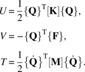
As mentioned before, the stiffness and mass matrices are independent of time. Therefore, these matrices need to be constructed once. However, the applied load vector is given as a function of time, and accordingly, the vectors of nodal DOFs and velocities are also a function of time.
We use the Lagrange equations2 to derive the finite element equations of motion. Similar to the total potential energy in chapter 2, the Lagrangian is defined for a dynamic problem as ![]() . For an N DOF system, the Lagrange equations are given by
. For an N DOF system, the Lagrange equations are given by

Note that the Lagrange equations consider that {Q} and ![]() are independent. Therefore, only the kinetic energy term is involved in
are independent. Therefore, only the kinetic energy term is involved in ![]() , while the strain energy and the potential energy of the external loads are involved in
, while the strain energy and the potential energy of the external loads are involved in ![]() . By substituting for all three energy terms of L from eq. (8.9) into eq. (8.10), we obtain the following dynamic finite element equations of motion:
. By substituting for all three energy terms of L from eq. (8.9) into eq. (8.10), we obtain the following dynamic finite element equations of motion:
In the above equation, ![]() is the vector of global nodal accelerations. Since the acceleration is the second‐order derivative of the displacement, the above equation is the system of second‐order differential equations with respect to time. Methods for solving the above equations will be discussed in the rest of this chapter.
is the vector of global nodal accelerations. Since the acceleration is the second‐order derivative of the displacement, the above equation is the system of second‐order differential equations with respect to time. Methods for solving the above equations will be discussed in the rest of this chapter.
The equation of motion in eq. (8.11) is the second‐order differential equation with respect to time. In order to solve for the differential equation, it is necessary to provide the initial conditions for the vectors of nodal displacements and velocities:

In addition to the initial conditions, the differential equations also need boundary conditions as with the static problems. In general, the boundary conditions are assumed independent of time. It is also assumed that the boundary conditions are given only for displacements. When the displacement is fixed, then the velocity and acceleration are automatically vanish. It is possible to have a prescribed motion, that is, the displacement, velocity or acceleration on the boundary are given as a function of time. However, the prescribed motion will not be considered here.
Unlike static problems, dynamic problems may or may not have displacement boundary conditions. If there is no displacement boundary conditions, the structure will have a rigid‐body motion with deformation, such as a flying airplane. In such a case, both the rigid‐body motion and deformation are a function of time.
In general, the stiffness matrix, [K], and mass matrix, [M], are independent of time when the deformation is small. Therefore, they are calculated at the initial time and repeatedly used. The force, {F(t)}, is given as a function of time.
8.2.2 Lumped Mass Matrix of a Uniaxial Bar Element
As mentioned in the previous section, the consistent mass matrix is derived by equating the kinetic energy of the bar, a continuous system, to that of the finite element model, a discrete system, using the shape functions. Therefore, the derived mass matrix is consistent with the finite element interpolation scheme. It is noted that the consistent mass matrix is fully populated like the element stiffness matrix. There is another simpler heuristic way of deriving the mass matrix. In this method, the mass of the element is distributed equally between the two nodes. That is, all mass is placed at the nodes, and the bar is supposed to possess only elasticity. This is similar to a discrete spring‐mass system discussed in chapter 1 (see figure 8.2).

Figure 8.2 Lumped mass idealization of a uniaxial bar element
In the lumped mass assumption, the kinetic energy of the element is the sum of the kinetic energies of the two concentrated masses placed at the nodes:
Note that the term ρAL is the mass of the element. The above expression can be written in a matrix form as

where ![]() is called the lumped mass matrix. Note that the sum of all components of the lumped mass matrix is equal to the mass of the bar element, which is the same as the consistent mass matrix. The lumped mass matrix is also positive definite. The consistent mass matrix assumes that the mass is distributed throughout the element, while the lumped mass matrix assumes that the mass is concentrated at the nodes.
is called the lumped mass matrix. Note that the sum of all components of the lumped mass matrix is equal to the mass of the bar element, which is the same as the consistent mass matrix. The lumped mass matrix is also positive definite. The consistent mass matrix assumes that the mass is distributed throughout the element, while the lumped mass matrix assumes that the mass is concentrated at the nodes.
As can be seen in eq. (8.14), the lumped mass matrix of an element is a diagonal matrix. If the element mass matrix is diagonal, the global mass matrix after assembly will also be diagonal. Many numerical advantages exist when the global mass matrix is diagonal. Therefore, it would be important to understand how much accuracy may be lost and how much numerical advantage may be achieved by using the lumped mass matrix.
8.2.3 Mass Matrix of a Beam Element
As the first step in the dynamic analysis of beam elements, we will derive the mass matrix for a beam element. Consider a generic beam element discussed in section 3.3. The deflection of the beam in terms of nodal DOFs and shape functions is given in eq. (3.44). The kinetic energy of the beam can be written as

where ![]() is the transverse velocity of the vibrating beam. The above expression for kinetic energy is consistent with the Euler‐Bernoulli beam theory described in chapter 3. Even though the rotation of the cross section of the beam also contributes to the rotational kinetic energy, it is neglected in the current formulation as it is considered small compared to the kinetic energy due to transverse motion. The velocity can be derived in terms of nodal DOFs as
is the transverse velocity of the vibrating beam. The above expression for kinetic energy is consistent with the Euler‐Bernoulli beam theory described in chapter 3. Even though the rotation of the cross section of the beam also contributes to the rotational kinetic energy, it is neglected in the current formulation as it is considered small compared to the kinetic energy due to transverse motion. The velocity can be derived in terms of nodal DOFs as
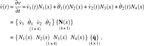
where {N(x)} and ![]() , respectively, are the column vectors of shape functions and the nodal velocities corresponding to the four DOFs of beam element. Even if the shape functions are written as a function of coordinate x, the shape functions of beam elements in eq. (3.43) were given in terms of parametric coordinate s, as
, respectively, are the column vectors of shape functions and the nodal velocities corresponding to the four DOFs of beam element. Even if the shape functions are written as a function of coordinate x, the shape functions of beam elements in eq. (3.43) were given in terms of parametric coordinate s, as

with the relationship of s = x/L. Substituting for ![]() from eq. (8.16) into eq. (8.15) and following the steps used in deriving the mass matrix for uniaxial bar elements, the components of the consistent mass matrix can be defined as
from eq. (8.16) into eq. (8.15) and following the steps used in deriving the mass matrix for uniaxial bar elements, the components of the consistent mass matrix can be defined as

Substituting for Ni(s) from eq. (8.17) and evaluating the integrals, we obtain the consistent mass matrix of a beam element as

Unlike the consistent mass matrix of the bar element, it is not straightforward to interpret the consistent mass matrix of the beam element. Some components even have a negative value. This is because the beam element has both translational DOFs (v1 and v2) and rotational DOFs (θ1 and θ2). However, if the components of translational DOFs are added, it is the same as the mass of the beam element: (156 + 54 + 54 + 156) × ρAL/420 = ρAL. Again, like the bar element, the consistent mass matrix of the beam element is also positive definite.
The kinetic energy of a beam element is then given by
Assembling of element mass matrices to obtain the global mass matrix follows similar procedures as before.
8.2.4 Lumped Mass Matrix for a Beam
In the case of the bar element, the lumped mass matrix is obtained by assuming that the mass of the element is distributed equally between the two nodes. In the case of beam element, however, this is not straightforward, as the beam element has rotational DOFs. In deriving the lumped mass matrix of the beam element, we assume the same lumped mass distribution in figure 8.2. Therefore, the components of mass matrix corresponding to the translation DOFs (v1 and v2) are the same as that of the bar element that is, a half of mass to each DOF. For rotational DOFs (θ1 and θ2), the mass moment of inertia is used. When a mass of ρAL/2 is located at the distance of L/2, the mass moment of inertia becomes I = (ρAL/2) × (L/2)2/3 = ρAL3/24. Therefore, the lumped mass matrix of the beam element can be defined as

8.3 NATURAL VIBRATION: NATURAL FREQUENCIES AND MODE SHAPES
A system is said to undergo natural vibration when it oscillates in one of its natural or fundamental modes of vibration. For example, when a mass‐spring system is stretched from its undeformed position and released, it will oscillate at its natural frequency. All dynamics systems, such as a vibrating structure, have certain preferred or fundamental modes of vibration. For discrete systems, the number of fundamental modes is equal to the number of degrees of freedom of the system. In this section, we will study modal analysis approach (also known as frequency analysis) for computing the natural modes of vibration of structures. When a structure is vibrating in one of its fundamental modes, it vibrates at a frequency that is unique to that mode of vibration. The frequency of a fundamental mode of vibration is called its natural frequency, which is an important dynamic characteristic of the system. To understand the dynamic characteristics of a system, we need to know its natural frequencies and mode shapes that together describe the natural vibration modes of the system. In the study of natural vibrations, the effect of damping is often ignored to understand the dynamic characteristics of the system. In this section, a simple one‐dimensional mass‐spring system is introduced first, in order to derive the dynamic equation of free vibration, followed by the system of matrix equations for finite element models.
8.3.1 Natural Vibration of One‐Dimensional Mass‐Spring System
In this section, a simple mass‐spring system is considered to derive the dynamic equation of free vibration. For free vibration, it is assumed that the damping is negligible and that there is no external force applied to the mass. Referring to figure 8.3, the only force applied to the mass is from the deformation of spring, as
where k is the spring constant in the units of force/displacement (e.g., lb/in or N/m). The negative sign indicates that the force is always opposing the motion of the mass attached to it. Based on Newton’s second law of motion, the force applied to the mass is proportional to the acceleration of the mass as given by
By substituting from eq. (8.22), the following ordinary differential equation can be obtained:
This is the dynamic equation for free vibration for one‐dimensional mass‐spring system. Note that this equation has a similar form as eq. (8.11) when the external force is zero. It will be shown in the next section that a similar equation but with a higher dimension can be obtained for the finite element model with multiple degrees of freedom.

Figure 8.3 Free vibration of 1D spring‐mass system
If the spring is initially stretched by magnitude A and then released, the solution to the above free vibration equation that describes the motion of mass becomes (see figure 8.4)
This solution says that it will oscillate with simple harmonic motion that has an amplitude of A and a frequency of fn (units of Hz). The value fn is called the undamped natural frequency. For the simple mass–spring system, fn is defined as

where T is the period of oscillation (seconds). The natural frequency can also be represented using the angular velocity (units of rad/sec) ![]() .
.
If the mass and stiffness of the system is known, the formula above can determine the frequency at which the system vibrates once set in motion by an initial disturbance. The system will vibrate slowly if the mass is increased or the stiffness is decreased. Every vibrating system has one or more natural frequencies that it vibrates at once disturbed. This simple relation can be used to understand in general what happens to a more complex system once we add mass or stiffness.

Figure 8.4 Free vibration of 1D mass‐spring system
An interesting observation is that the natural frequency is independent of the initial perturbation, but the amplitude depends on it. That is, no matter what amplitude is applied for the initial perturbation, the system will oscillate in the same natural frequency, which means that the natural frequency is a system‐related characteristic. In fact, in the free vibration analysis, the initial perturbation is assumed arbitrary, and the natural frequency is the main interest.
The natural frequency is important when designing a system under dynamic loads. If the excitation frequency of the applied load is the same as the natural frequency of the system, then a phenomenon called resonance occurs. At resonant frequencies, small periodically applied forces have the ability to produce large amplitude oscillations, which can cause a catastrophic failure of the system. Therefore, it is important for engineers to identify all natural frequencies of the system and to make sure that the excitation frequencies of applied loads are not close to the natural frequencies.
8.3.2 Natural Vibration Analysis Using Finite Element Models
As explained in the previous section, the dynamic equation of natural vibration of a finite element model can be obtained from eq. (8.11) by removing the externally applied forces. Therefore, the dynamic equation of natural vibration for finite element model can be written as
The detailed expression of this equation for a bar, a beam, and the system of springs will be given in examples. Since the nodal DOFs of finite elements will undergo a harmonic motion under free vibration, it is possible to assume the following form of nodal DOFs:
where {A} = {A1, A2,…AN}T is a vector of unknown constants, and ω is the angular velocity of periodic motion. Physically Ai is the amplitude of vibration of the i‐th DOF.
An interesting observation from eq. (8.28) is that the vibration response {Q(t)} is decomposed into a constant deformation mode and a time‐varying part. If the vector {A} is considered as nodal displacements, it represents the shape of deformation (or mode shape) during the vibration. On the other hand, the time‐varying term, eiωt, varies between +1 and −1 to represent the oscillatory motion. Therefore, the finite element model will vibrate with the shape of {A} and the frequency of ![]() Hz. The vector {A} is called the mode shape and fn is called the natural frequency. Since the mode shape depends on the initial perturbation, its magnitude is not of interest; it is often normalized. Note that even though {A} = {0} satisfies the dynamics equation in eq. (8.27), it is called a trivial solution because there is no vibration. So we are looking for a nontrivial solution with {A} ≠ {0}.
Hz. The vector {A} is called the mode shape and fn is called the natural frequency. Since the mode shape depends on the initial perturbation, its magnitude is not of interest; it is often normalized. Note that even though {A} = {0} satisfies the dynamics equation in eq. (8.27), it is called a trivial solution because there is no vibration. So we are looking for a nontrivial solution with {A} ≠ {0}.
Although we have defined mode shapes and natural frequencies, they are still unknown quantities to be determined. We will now describe a standard approach called modal analysis for computing these quantities where the assumed solution in eq. (8.28) is substituted into the equations of motion in eq. (8.27) to yield an eigenvalue problem.

One can recognize the above as the generalized eigenvalue problem in which ω2 is the eigenvalue and {A} is the corresponding eigenvector (see section A.4 of the appendix). The physical meaning of the above equation is as follows. The equations of motion have nontrivial solutions for only certain values of ω for which the determinant of the matrix vanishes; that is,
Otherwise, the solution of the set of equations is {A} = {0}. That means there is no motion or vibration, which is a trivial solution. In general, the number of natural frequencies is the same as the number of DOFs of the system. Therefore, theoretically, there are N number of natural frequencies and mode shapes: (ω1, {A(1)}), (ω2, {A(2)}), …, (ωN, {A(N)}).
For a given eigenvalue ![]() , eq. (8.29) is solved for the corresponding eigenvector {A(i)}. However, since the determinant of the coefficient matrix is zero, eq. (8.29) may yield infinitely many solutions. That is, if {A(i)} is a solution to eq. (8.29), then α{A(i)} can also be a solution for an arbitrary α. Therefore, among infinitely many solutions, the one that satisfies a condition is used as an eigenvector. For example, it is possible to choose the eigenvector whose magnitude is one; that is,
, eq. (8.29) is solved for the corresponding eigenvector {A(i)}. However, since the determinant of the coefficient matrix is zero, eq. (8.29) may yield infinitely many solutions. That is, if {A(i)} is a solution to eq. (8.29), then α{A(i)} can also be a solution for an arbitrary α. Therefore, among infinitely many solutions, the one that satisfies a condition is used as an eigenvector. For example, it is possible to choose the eigenvector whose magnitude is one; that is, ![]() . Imposing the condition that the eigenvector has unit magnitude is called normalization. In fact, normalization is commonly used in solving standard eigenvalue problems. In the case of generalized eigenvalue problems, as in free vibration problems, the eigenvectors are normalized by using the mass matrix; that is, eigenvectors are chosen such that
. Imposing the condition that the eigenvector has unit magnitude is called normalization. In fact, normalization is commonly used in solving standard eigenvalue problems. In the case of generalized eigenvalue problems, as in free vibration problems, the eigenvectors are normalized by using the mass matrix; that is, eigenvectors are chosen such that ![]() . This choice of normalization does not have any physical meaning; rather it is more of computational convenience.
. This choice of normalization does not have any physical meaning; rather it is more of computational convenience.
If the structure is excited by an applied load with frequency of ω1, it will vibrate in the shape of {A(1)}, and so on. In general, however, excitation frequencies are much lower than the natural frequencies of the structure. Therefore, a handful of the lowest natural frequencies are of interest. Often, only the lowest natural frequencies are required in design. Therefore, many numerical algorithms in solving the eigenvalue problem only calculate the lowest n (n is much smaller than N) number of eigenvalues instead of calculating all eigenvalues, to reduce the computational cost.
So far, we only consider the cases when the displacement boundary conditions are given such that the rigid body motions are eliminated. However, it is possible that the generalized eigenvalue problem in eq. (8.29) can be solved in the structural matrix level; that is, before applying boundary conditions. In such a case, the structural stiffness matrix is positive semi‐definite and will have zero eigenvalues. The number of zero eigenvalues is the same as the number of rigid body motions. For example, in the case of a uniaxial bar, there is one rigid body motion, while there are two rigid body motions for plane beams. Therefore, when the structure has rigid body motions, the zero eigenvalues should not be used in calculating the natural frequencies of the structure.
As a closing remark, it is emphasized again that the natural vibration analysis does not require any externally applied loads. Natural vibration analysis is related to the vibration characteristics of the system, not to the applied loads or initial conditions. The magnitude of mode shapes (eigenvectors) do not have any physical meaning; their shapes are the mode of vibration when the system is excited at the corresponding frequency. When the applied load is composed of the combination of multiple frequencies, the system will also respond as the combination of multiple mode shapes, which requires a method called mode superposition. This will be discussed further in section 8.5.
8.4 FORCED VIBRATION: DIRECT INTEGRATION APPROACH
When time‐dependent loads and/or boundary conditions are applied to the structure, the dynamic response of the structure becomes important, and inertial effects and wave propagation are dominant throughout the structure compared with the quasi‐static response. Time history analysis is concerned with computing the response of the structure under time‐dependent loads. In general, the methods of analysis can be classified into two broad categories: the direct integration method and the mode superposition method. In the direct integration method, the ordinary differential equations are integrated using a step‐by‐step numerical procedure. There is no transformation of the finite element matrix equation. In the mode superposition method, on the other hand, the finite element matrix equation is transformed so that the solution space is spanned by the eigenvectors of the system. The unknown displacements are represented as a linear combination of the mode shapes. The direct integration method will be explained in this section, while the mode superposition method will be discussed in section 8.5.
In chapter 2, we showed that the static equilibrium of a structure could be written as partial differential equations whose weighted residual becomes the finite element matrix equation after discretization. This is in fact the partial differential equation over the structural space. The dynamic equation is an ordinary differential equation over time. Unlike partial differential equations, the dynamic equation is often solved using finite difference methods. While partial differential equations have boundary conditions, ordinary differential equations have initial conditions at t = 0.
In the finite difference methods, the continuous time interval [0, T] is discretized by [t0 = 0, t1, t2, …, tn, …, tN = T] first, and then, the equilibrium equation in eq. (8.11) is imposed at each discrete time. It is possible that the time increment can be variable, but it is assumed that a constant time increment is used; that is, ![]() . Let the current time be tn. Then, the dynamic equilibrium equation can be written as
. Let the current time be tn. Then, the dynamic equilibrium equation can be written as
where ![]() . Our goal is to determine {Q(t)} and thus
. Our goal is to determine {Q(t)} and thus ![]() given the initial conditions of the nodal DOFs and the forcing functions {F(t)}. In the discretized time intervals, it is equivalent to determining {Qn} and
given the initial conditions of the nodal DOFs and the forcing functions {F(t)}. In the discretized time intervals, it is equivalent to determining {Qn} and ![]() . In the following derivations, we assume that the dynamic problem has been solved up to time tn, and the solution at tn+1 is required.
. In the following derivations, we assume that the dynamic problem has been solved up to time tn, and the solution at tn+1 is required.
The typical solution procedure of the direct integration method is calculating the unknown nodal displacements, velocities, and acceleration at time tn+1 based on known information from the previous times, tn, tn−1, and so forth. If the integration method only requires the information from previous time tn, it is called a one‐step method; if it requires more than one previous times, it is called a multi‐step method. In addition, if the displacements, velocities, and accelerations at tn+1 are expressed in terms of those at tn or previous times, then it is called an explicit method. On the other hand, if the method requires information at tn+1, then it is called an implicit method. The implicit method requires solving a system of equations to calculate the information at time tn+1, and therefore, it is more expensive than the explicit method. However, in general, larger time‐step size can be used for an implicit method than for an explicit method in order to satisfy the stability condition.
The key concept of the direct integration methods is to approximate the time derivatives, ![]() and
and ![]() using finite differences. Different methods have been proposed depending on how the time derivatives are approximated. Since the accuracy and stability of the solution depend on the method of choice, it is important for the users to fully understand the characteristics of different time integration methods. In this section, some commonly used methods are presented. The advantages and limitations of various methods will be discussed.
using finite differences. Different methods have been proposed depending on how the time derivatives are approximated. Since the accuracy and stability of the solution depend on the method of choice, it is important for the users to fully understand the characteristics of different time integration methods. In this section, some commonly used methods are presented. The advantages and limitations of various methods will be discussed.
8.4.1 Implicit versus Explicit Time Integration Methods
In general, various time integration methods for ordinary differential equations can be categorized either as explicit methods or implicit methods. When a direct computation of the field variables can be made in terms of known quantities, the computational method is called an explicit method. When the field variables are defined by coupled sets of equations, and either a matrix or an iterative technique is needed to calculate the variable, the numerical method is called an implicit method. In general, the explicit method is computationally less expensive during each step but requires many more time steps because it requires a very small time step in order to make the numerical integration stable. On the other hand, many implicit methods are stable no matter what time step is used. However, if the time step is too large, the numerical method may not be accurate. Therefore, an appropriate time‐step size should be used by considering both accuracy and stability.
Explicit method: The simplest method of explicit time integration is the forward Euler method, which is used to solve first‐order ordinary differential equations. Although we are interested in the second‐order ordinary differential equation in eq. (8.31), we will use the first‐order differential equation to explain the difference between the implicit and explicit methods. Consider that we want to solve the following differential equation with the initial condition ![]() in the time interval [0, T]:
in the time interval [0, T]:
In the numerical time integration approach, the above differential equation is solved at a discrete set of times. Let the continuous time interval be discretized by [t0 = 0, t1, t2, …, tn, …, tN = T]. As the initial condition is given at t0, we want to use the information at t0 to calculate the information at t1. If we repeat this process, we can solve for information at all discrete times.
The forward Euler method is based on the first‐order Taylor series expansion with respect to tn. To determine y(tn+1) = yn+1, the following integration rule can be obtained:
Since y(tn) = yn is already calculated at the previous time, and the function f(tn,yn) is available, all the terms on the right‐hand side of eq. (8.33) are known. Therefore, the unknown variable yn+1 can be explicitly calculated using the information from the previous time step.
The numerical integration formula in eq. (8.33) can be viewed as an approximation of the time derivative ![]() . That is, in the forward Euler method, the time derivative is approximated by
. That is, in the forward Euler method, the time derivative is approximated by
The explicit method calculates the system response at the next time from the state of the system at the current time, which is why it is called a “forward” difference method.
Implicit method: Unlike the explicit method, the implicit method calculates the system response at the next time by solving an equation involving both the current and next times. For example, the counter‐part of the forward Euler method is the backward Euler method, which can be written as
If f(t, y) is a nonlinear function of y, an iterative approach is required to solve the implicit time integration. Even if we showed only two cases of evaluating f(t, y) at tn and tn+1 to approximate the time derivative, it is possible that it can be generalized to ![]() , where
, where ![]() . Many different numerical methods are based on this generalization.
. Many different numerical methods are based on this generalization.
Even if the implicit method requires iteration, it has an advantage of stability. That is, eq. (8.35) is unconditionally stable no matter what size of time step Δt is used. On the other hand, eq. (8.33) is conditionally stable, which requires a relatively small time step. However, if a large time step is used for the implicit method, the accuracy of the approximation will be sacrificed.
8.4.2 Central Difference Method: Explicit Time Integration
In the central difference method (CDM), the velocity and acceleration are approximated as

where the subscript n denotes time step ![]() and
and ![]() . Note that the curly brackets for a vector are omitted for the simplification of notation. In approximating acceleration in eq. (8.37), the velocity is calculated using the forward Euler method in eq. (8.34). Therefore, the velocity and acceleration are calculated using different schemes in CDM. Then, the equilibrium is applied at tn as
. Note that the curly brackets for a vector are omitted for the simplification of notation. In approximating acceleration in eq. (8.37), the velocity is calculated using the forward Euler method in eq. (8.34). Therefore, the velocity and acceleration are calculated using different schemes in CDM. Then, the equilibrium is applied at tn as
Substituting for ![]() from eq. (8.37) into the above equation and rearranging the terms, we obtain
from eq. (8.37) into the above equation and rearranging the terms, we obtain
Note that we use the displacements at the n‐th and (n − 1)‐th time steps in order to solve for displacements at the (n + 1)‐th step. That is, in order to calculate the displacement at a new time step, only information at the previous time steps is required. Since information at the previous time steps is already available, the unknown displacement at a new step is an explicit function of information from the previous steps. That is why the central difference method is called an explicit method.
It is noted that the inverse of the mass matrix is required to calculate the displacement in eq. (8.39). If the lumped mass matrix is used, then the inverse is trivial. Therefore, the CDM is computationally efficient with the lumped mass matrix. By careful implementation, it is unnecessary to build the global stiffness matrix [K]. The calculation can be done in the element level.
The central difference method is also called a two‐step method because the displacements at two consecutive time steps, (n − 1) and n, are used to determine displacements at (n + 1)‐th step. This can cause an issue to calculate the displacement at t1 because in order to determine Q1 we need the initial condition Q0, and also Q−1. The steps involved in the CDM are listed below:
- The initial acceleration can be calculated from the equations of motion in eq. (8.38) as(8.40)

- By using Taylor series expansion, we obtain(8.41)

- By substituting for initial conditions in the above equation, Q−1 can be calculated. Knowing the displacements at n = −1 and n = 0, one can calculate Q1 using eq. (8.39) as:(8.42)

- Knowing Q0 and Q1, use eq. (8.39) to calculate Qn for n = 2, 3, …, iteratively.
Once displacement Qn+1 at tn+1 is calculated, the velocity and acceleration at time tn can be calculated using eq. (8.36) and (8.37). Note that the velocity and acceleration are calculated one step behind than the displacement. That is, after calculating displacement Qn+1, the velocity and acceleration at tn are updated. Another method of starting the CDM is to use one of the implicit methods described in the next section to calculate Q1 as accurately as possible and proceed to step 4 above to use the CDM.
The CDM is the simplest of all direct integration methods. First, it is unnecessary to factorize the stiffness matrix as in the quasi‐static problem. Only the mass matrix needs to be factorized. If the lumped mass matrix is used, then M will be diagonal, and calculating M−1 in eq. (8.39) is straightforward and computationally efficient. However, CDM is only conditionally stable. To ensure stability, the time step Δt must be less than a critical value Δtcr. The critical value of Δt is given as6
where ωmax is the highest natural frequency of the finite element model. In general, ωmax increases as the element size decreases or the stiffness of the material increases. Therefore, when small‐sized elements are used with a highly stiff material, a very small time step must be used to make the explicit time integration stable.
As mentioned before, the central difference method is easy to implement because the variables at time tn+1 are an explicit function of variables at time tn. However, the method is conditionally stable; that is, it requires a small time step to be stable. In order to show the issue related to instability, the same problem in example 8.5 is solved with a larger time step. As we calculated in example 8.5, the critical time step is ![]() . Therefore, we solved the same problem with
. Therefore, we solved the same problem with ![]() , whose results are shown in figure 8.11. In the figure, a small oscillatory error starts in early time, and then, the error exponentially increases in the following time and eventually diverged. Therefore, it is important to keep the time step smaller than the critical time step. In order to be conservative, often the time step is chosen much smaller than the critical time step.
, whose results are shown in figure 8.11. In the figure, a small oscillatory error starts in early time, and then, the error exponentially increases in the following time and eventually diverged. Therefore, it is important to keep the time step smaller than the critical time step. In order to be conservative, often the time step is chosen much smaller than the critical time step.

Figure 8.11 Instability of the central finite difference method due to a large time step
It would be also interesting to solve the same problem in example 8.5, but this time with a slow application of the load. In order to do that, tmax = 30 ms is used. Note that even if the ending time is increased by 10 times, the time step needs to remain the same as ![]() in order to maintain stability. Figure 8.12 shows the results from the central difference method and from the quasi‐static solution. It is interesting to note that there is no significant difference between the dynamic and quasi‐static analysis results. As shown in example 8.5, the period of vibration for the bar is about 0.8 ms; that is, the bar can vibrate about 1.26 cycles in a millisecond. Therefore, if the applied load is in the order of 10 ms, the load is relatively slow compared to the structure’s natural vibration frequency. Therefore, the structure behaves as if it were under a quasi‐static load.
in order to maintain stability. Figure 8.12 shows the results from the central difference method and from the quasi‐static solution. It is interesting to note that there is no significant difference between the dynamic and quasi‐static analysis results. As shown in example 8.5, the period of vibration for the bar is about 0.8 ms; that is, the bar can vibrate about 1.26 cycles in a millisecond. Therefore, if the applied load is in the order of 10 ms, the load is relatively slow compared to the structure’s natural vibration frequency. Therefore, the structure behaves as if it were under a quasi‐static load.

Figure 8.12 Equivalence of dynamic and static solution under slowly applied load
8.4.3 Newmark Method: Implicit Time Integration
In the implicit methods, we apply the equations of motion in eq. (8.38) at time step (n + 1) in order to calculate the displacements Qn+1. This is different from the explicit CDM wherein the equations were applied at the previous time step n. The Newmark family of time integration algorithms is one of the most popular time integration methods as a single‐step algorithm. Consider the following Taylor series expansions for velocity:
and displacement:
where γ and β are two parameters that determine the accuracy and stability of integration. Note that when ![]() , the Newmark integration method becomes an explicit method. Therefore, in the following derivations, we assume that
, the Newmark integration method becomes an explicit method. Therefore, in the following derivations, we assume that ![]() . The Newmark family of algorithms are based on different choices of these parameters. Some common algorithms will be presented later.
. The Newmark family of algorithms are based on different choices of these parameters. Some common algorithms will be presented later.
The Newmark algorithm can be split into two steps: predictor and correction steps. In the predictor step, the velocity and displacement are predicted using known information at time tn. After calculating the acceleration at time tn+1, the corrector step updates the velocity and displacement with the acceleration. From eqs. (8.44) and (8.45), the predictors for velocity and displacement are defined as
That is, the predictors include those terms at time tn. Once the acceleration at time tn+1 is given, they are corrected as
Therefore, the only remaining task is to calculate the acceleration at time tn+1, which can be achieved by substituting eq. (8.49) into the equations of motion in eq. (8.38) at tn+1:
Substituting for ![]() from eq. (8.49) into the above equation and rearranging the terms we obtain
from eq. (8.49) into the above equation and rearranging the terms we obtain
where the effective mass matrix and load vector are derived as

Note that the Newmark method solves for acceleration in eq. (8.51), while the central difference method in section 8.4.2 solves for displacement. In general, it is possible that the Newmark method can be formulated to solve for displacement, which is left as an exercise problem. Once the acceleration is calculated, the velocity and displacement can be corrected using eqs. (8.48) and (8.49).
The steps involved in implementing Newmark’s method are summarized below. We note that there is no need for any special starting procedure, which was required in the case of the central difference method.
- Calculate the initial acceleration using

- Construct the effective mass matrix

- Set n = 0, and calculate predictors:


- Construct the effective force vector

- Solve for


- Correct velocity and displacement


- If n = N, stop. Otherwise, set n = n + 1 and go to step 3
As mentioned before, the performance of Newmark integration algorithms depend on the choice of the two parameters, γ and β. The most important factors in choosing appropriate parameters are accuracy, stability, and dissipation. Accuracy and stability of a numerical integration were explained when we discussed the central difference method. When a numerical solution is approximated, the energy of the initial wave may be reduced in a way analogous to a diffusional process, which is called numerical dissipation. In some cases, “artificial dissipation” is intentionally added to improve numerical stability of the solution. Some combinations of γ and β may or may not include the numerical dissipation. Table 8.1 shows some examples of the Newmark family time integration algorithms.
Table 8.1 Newmark family of time integration algorithms
| Method | γ | β | Properties |
| Average acceleration | 1/2 | 1/4 | Implicit, unconditionally stable |
| Linear acceleration | 1/2 | 1/6 | Implicit, conditionally stable |
| Fox‐Goodwin | 1/2 | 1/12 | Implicit, conditionally stable. 4th‐order accuracy |
| Central difference | 1/2 | 0 | Explicit, conditionally stable |
In conditionally stable time integration algorithms, such as the central difference method, stability is affected by the size of the time step. Normally, if the chosen time step that can provide stability is small enough, accuracy is not a major issue for the conditionally stable algorithms. In unconditionally stable time integration algorithms, however, a time step size can be chosen independent of stability considerations. Therefore, the size of the time step in unconditionally stable algorithms can be much larger than that of the conditionally stable algorithms. However, the size of the time step must be chosen to provide the required level of accuracy because the accuracy decreases as the size of time step increases.
Advanced studies on stability and accuracy using eigenvalue analysis show that the Newmark family methods show second‐order accuracy with ![]() , while they show first‐order accuracy when
, while they show first‐order accuracy when ![]() . Since accuracy is an important criterion, many Newmark family algorithms use
. Since accuracy is an important criterion, many Newmark family algorithms use ![]() . However, numerical damping does not provide stability for
. However, numerical damping does not provide stability for ![]() . Therefore, for Newmark methods,
. Therefore, for Newmark methods, ![]() is necessary to introduce high‐frequency dissipation.
is necessary to introduce high‐frequency dissipation.
For stability, the same eigenvalue analysis shows that the Newmark method has the following stability conditions:
For conditionally stable algorithms, the time step should be less than the critical time step. For the undamped system, the critical time step, Δtcr, can be calculated by

where ωmax is the largest eigenvalue of the system. In general, the element eigenvalue is larger than that of the system. Since the maximum eigenvalue of the system is difficult to calculate, the maximum element eigenvalue is often used as a conservative estimate. Let the element size be L. It is also beneficial to note that the maximum element eigenvalue is ![]() . Therefore, as the element size is decreased, the critical time step also decreases.
. Therefore, as the element size is decreased, the critical time step also decreases.
8.5 METHOD OF MODE SUPERPOSITION
The direct integration method discussed in section 8.4 is most suitable when the loads act over a short duration, and only the response during the same short duration is of crucial interest. Since the time step required is very small, direct integration methods are not suitable when the response is required for a long period. In such a case, we propose to identify a transformation of displacements that will enable us to make the solution technique very efficient for a long‐duration response.
As explained in section 8.3, structures vibrate at their natural frequencies when their natural modes of vibration are excited. If the excitation frequency of the applied force is much smaller than the lowest natural frequencies of the structure, it will behave as if a quasi‐static load is applied. On the other hand, if the excitation frequency is the same as one of the natural frequencies, a phenomenon called resonance occurs, and the amplitude of vibration greatly increases and can cause structural failure. Since the structure vibrates in its mode shapes, it is possible to express the forced vibration response of a structure as a linear combination of its mode shapes, which allows us to decouple the equation of motion. This approach for computing the forced response of structure is called the method of mode superposition. In fact, the method of mode superposition is commonly used in forced vibrations of linear systems because it can provide insight into the structure’s behavior that is not otherwise available and because it is usually significantly more cost effective than the direct time integration methods.
Before we proceed further, we will derive certain properties of eigenvectors. Consider the generalized eigenvalue problem in eq. (8.29), which can be written as
As we noted earlier, for an N‐DOFs system, the above eigenvalue problem leads to N natural frequencies, ω1, ω2, …, ωN, and corresponding eigenvectors A1, A2,…, AN. Each eigenvalue and its eigenvector must satisfy the above equation. Let us consider such equations for two arbitrary modes i and j:

We multiply the first equation by ![]() and the second by
and the second by ![]() and subtract to obtain:
and subtract to obtain:
In arriving at the above equation, we have used the identities ![]() and
and ![]() because K and M are symmetric matrices. From eq. (8.58) we find that when
because K and M are symmetric matrices. From eq. (8.58) we find that when ![]() , that is,
, that is, ![]() ,
, ![]() must be equal to zero. That is, the eigenvectors are orthogonal in some sense, and we call them M‐orthogonal. Now consider the case i = j. The product
must be equal to zero. That is, the eigenvectors are orthogonal in some sense, and we call them M‐orthogonal. Now consider the case i = j. The product ![]() must be positive if it is nonzero, because M is positive definite. Let us denote the product by
must be positive if it is nonzero, because M is positive definite. Let us denote the product by ![]() . Then we can normalize the eigenvector by dividing by ri such that
. Then we can normalize the eigenvector by dividing by ri such that ![]() . Then from eq. (8.57), it follows that
. Then from eq. (8.57), it follows that ![]() . Thus, the properties of the eigenvectors can be summarized as:
. Thus, the properties of the eigenvectors can be summarized as:

Let us define a square matrix Λ whose columns are the eigenvectors Aj. That is

where ![]() is the m‐th DOF of n‐th eigenvector. Then from eq. (8.59), we can deduce the following:
is the m‐th DOF of n‐th eigenvector. Then from eq. (8.59), we can deduce the following:
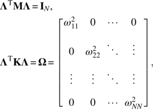
where IN is the ![]() identity matrix. Note that
identity matrix. Note that ![]() is a diagonal matrix of eigenvalues.
is a diagonal matrix of eigenvalues.
8.5.1 Modal Decomposition
Returning to forced vibration problems, our goal is to simplify the time integration procedures. As we mentioned before, the response of forced vibration can be represented using a linear combination of mode shapes. That is, the dynamic response can be written as
where the mode shapes are independent of time, while the vector of coefficients, {X(t)} = {x1(t), x2(t), …, xN(t)}T, are a function of time. Therefore, the shape of deformation is determined by mode shapes, while the time‐varying magnitude of deformation is represented by {X(t)}.
Since eigenvectors are M‐orthogonal based on the discussion in eq. (8.59), they can be considered as modal basis vectors. Then, the above modal decomposition can be considered as a transformation from physical DOFs {Q(t)} to modal DOFs {X(t)}, as
Substituting the transformation in eq. (8.31), we obtain the equation of motion as:
That is, instead of solving physical DOFs, the transformed equation solves for the modal DOFs. This transformation to modal DOFs can provide significant computational efficiency. In practice, only a small number of modes are enough to accurately approximate the physical DOFs in eq. (8.62). That is, the number of modes N can be much smaller than the size of matrix.
The matrix equation in eq. (8.63) can be further simplified by pre‐multiplying the above equation by ![]() to obtain
to obtain
which can be written as
where ![]() is the generalized force vector given. From eq. (8.61), we note that
is the generalized force vector given. From eq. (8.61), we note that ![]() is an identity matrix, and
is an identity matrix, and ![]() is a diagonal matrix containing the squares of the natural frequencies, that is,
is a diagonal matrix containing the squares of the natural frequencies, that is, ![]() . Then the equations are completely decoupled and we obtain N number of differential equations as
. Then the equations are completely decoupled and we obtain N number of differential equations as
This is a significant simplification from the N‐dimensional system of coupled equations to N decoupled equations.
An analytical solution can be derived for eq. (8.66) and can be written as

The first two terms in this solution are referred to as the complementary solution, and it corresponds to the response if no external loads are acting. Therefore, the complementary solution is also called the free vibration response. The second part of the solution involves a convolution integral and is called the particular solution, which is the response of the structure to the external load. When damping is ignored, both of these components will last forever, but in reality there will be damping and the complementary part will be damped out so that only the particular part of the solution will continue as the steady‐state solution. The constants, Ai and Bi, are evaluated using the initial conditions of X, that is, X(0) and ![]() . The initial conditions are usually known for the nodal DOFs. Let the initial value of nodal variables and corresponding nodal velocities be represented as Q(0) and
. The initial conditions are usually known for the nodal DOFs. Let the initial value of nodal variables and corresponding nodal velocities be represented as Q(0) and ![]() . The inverse transformation corresponding to eq. (8.62) can be derived by pre‐multiplying the equation by ΛTM and using the orthogonality condition in eq. (8.59), as
. The inverse transformation corresponding to eq. (8.62) can be derived by pre‐multiplying the equation by ΛTM and using the orthogonality condition in eq. (8.59), as
Then, the initial conditions of X can be written as

Putting t = 0 in eq. (8.67), we obtain
Differentiating the solution for Xi(t) in eq. (8.67) and putting t = 0, we have

If the forcing function F(t) and hence R(t) are available in a closed form, then the integration above can also be performed in closed form. If the forcing function is known only in a discrete form, then numerical integration is used to evaluate the above integral. Once the solution is obtained for X(t), the solution in terms of nodal variables is obtained using the transformation ![]() (see eq. (8.62)).
(see eq. (8.62)).
8.6 DYNAMIC ANALYSIS WITH STRUCTURAL DAMPING
In the previous sections, we considered systems that have no damping. Now we will consider the implementation of damping in a spring‐mass‐dashpot (viscous damping) system shown in figure 8.18. The procedures are similar to the direct method of formulating the finite element equations described in section 1.1. Consider the free‐body diagram of a dashpot element in figure 8.18. The forces ![]() and
and ![]() can be related to the nodal velocities as
can be related to the nodal velocities as

or

Figure 8.18 One‐dimensional spring‐mass‐dashpot element
Recall that we have used a similar equation for spring elements of the form: ![]() in eq. (1.6). Now consider the equation of motion of a rigid mass at node i:
in eq. (1.6). Now consider the equation of motion of a rigid mass at node i:

where ie is the number of elements connected to node i. Note that the nodal forces ![]() can arise from a spring or damper (dashpot) or both. Substituting for
can arise from a spring or damper (dashpot) or both. Substituting for ![]() as a combination from eqs. (1.5) and (8.72), we obtain
as a combination from eqs. (1.5) and (8.72), we obtain

After deleting the rows and columns corresponding to zero DOFs, we obtain the equations of motion as:
The above equation can be solved using one of the time integration methods or the mode superposition method.
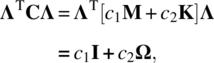
Damping in a continuous system is difficult to decouple. Hence, a heuristic method called proportional damping, also called Rayleigh damping, is used in practice. The damping matrix [C] is assumed to be a linear combination of stiffness and mass matrices as
where c1 and c2 are constants of proportionality. We make the proportional damping assumption mainly because it provides computational convenience.
8.6.1 Central Difference Method with Damping
Recall that in the CDM, the equilibrium condition is stated at time tn to calculate the displacements at time tn+1. We use central difference to approximate the velocity term in eq. (8.75):
Substituting for ![]() from eq. (8.37) and for
from eq. (8.37) and for ![]() from eq. (8.76) into (8.75) at time tn, and solving for
from eq. (8.76) into (8.75) at time tn, and solving for ![]() , we obtain
, we obtain

Since we know the right‐hand side, the above equation can be solved for ![]() . Note that the expression for
. Note that the expression for ![]() has to be modified as
has to be modified as
8.6.2 Newmark Method with Damping
As discussed earlier, the equilibrium is applied at time tn+1 in order to determine Qn+1:
When damping is included, the effective mass matrix and force vector in eq. (8.52) can be defined as

8.6.3 Modal Superposition with Damping
In the modal superposition method, we apply the transformation ![]() in eq. (8.62). Substituting the transformation in the equations of motion in eq. (8.75) and pre‐multiplying the equation by ΛT, we obtain
in eq. (8.62). Substituting the transformation in the equations of motion in eq. (8.75) and pre‐multiplying the equation by ΛT, we obtain
We have already shown that ![]() , and ΛTKΛ is a diagonal matrix consisting of squares of natural frequencies. Proportional damping allows the decoupling of the equations of motion in the modal superposition method as it did for the undamped cases.
, and ΛTKΛ is a diagonal matrix consisting of squares of natural frequencies. Proportional damping allows the decoupling of the equations of motion in the modal superposition method as it did for the undamped cases.
where I is an identity matrix of size ![]() and Ω is defined in eq. (8.61). Then we note that eq. (8.81) will decompose into N number of ordinary differential equations similar to eq. (8.66) but with an extra term for damping:
and Ω is defined in eq. (8.61). Then we note that eq. (8.81) will decompose into N number of ordinary differential equations similar to eq. (8.66) but with an extra term for damping:
where the damping ratio ξi is defined as (see (8.83))

The nature of the solution of equations (8.84) depends on the value of the damping ratios as shown below:
![]()

where ![]() . Here the first part of the solution is a convolution integral that corresponds to the forced response, and the second part is the complementary solution, which will die out due to damping, and is a transient response. After the transient solution dies out, only the particular solution exists as the steady‐state response. Note the frequency of the steady state response is slightly different from the natural frequency due to damping.
. Here the first part of the solution is a convolution integral that corresponds to the forced response, and the second part is the complementary solution, which will die out due to damping, and is a transient response. After the transient solution dies out, only the particular solution exists as the steady‐state response. Note the frequency of the steady state response is slightly different from the natural frequency due to damping.
![]()

When critical damping is present, the transient response or the complementary part does not have any oscillations. The steady‐state response, which is the particular solution, depends on the external load and will be periodic if the load is periodic.
![]()

where ![]() . In overdamped systems also, transient oscillations are suppressed entirely, and the system reaches steady state faster than critically damped systems. In the above solutions, ai and bi are constants to be determined from the initial conditions Xi(0) and
. In overdamped systems also, transient oscillations are suppressed entirely, and the system reaches steady state faster than critically damped systems. In the above solutions, ai and bi are constants to be determined from the initial conditions Xi(0) and ![]() . When the forcing function F(t) is not available in a closed form, numerical integration can be used. Procedures for numerical integration of eq. (8.84) can be found in many elementary books on vibration.8
. When the forcing function F(t) is not available in a closed form, numerical integration can be used. Procedures for numerical integration of eq. (8.84) can be found in many elementary books on vibration.8
8.7 FINITE ELEMENT MODELING PRACTICE FOR DYNAMIC PROBLEMS
The frequency for mode 5 is higher than the highest frequency component in the applied loads, and so we can reasonably assume that only these first five modes will be activated significantly by these two load cases. Figure 8.26 shows the deflection of the beam at A (x = 0.25 m) and B (x = 0.5 m) due to the single frequency load case (a). Note that the forcing frequency (100 Hz) is very close to the first natural frequency (105 Hz) and as a result, the amplitude of vibration increases quickly due to near‐resonant vibration. The shape of the response is the same at A and B, and they differ only in amplitude. Since the excitation frequency is close to mode 1, the shape of the response will be similar to that of the first mode.

Figure 8.26 Beam with deflection at A and B due to load (a)
The load defined in part (b) has multiple frequencies. For linear problems, such as this example, the dynamic response due to a load that contains multiple frequencies can be computed as a sum of the response from each frequency component acting separately.
Figure 8.27 shows the dynamic response of the beam to the load case (b). The dominant mode for this response is still the first mode due to the proximity of the first resonant frequency and the harmonic components of the load. As a result, the deflection due to this load looks somewhat similar to case (a), but the response to the load components with other frequencies are superimposed. The shape of the response is no longer identical for the two points A and B.

Figure 8.27 Beam with deflection at A and B due to load (b)
8.8 EXERCISES
- Answer the following descriptive questions.
- In the interpolation of displacement of a finite element,
 , which one depends on time and which one depends on domain?
 - Explain the difference between the consistent mass and lumped mass matrix.
- Will the natural frequency using lumped mass matrix be larger or smaller than the actual natural frequency? Explain why.
- If the mass of the system increases, will the natural frequency increase or decrease?
- If the stiffness of the system increases, will the natural frequency increase or decrease?
- Explain the difference between the eigenvalue problem and the generalized eigenvalue problem.
- Explain why the magnitude of mode shape is not important.
- If a 1D bar is modeled using 10 bar elements, when both ends of the bar are free, what would be the lowest natural frequency of the bar?
- If a numerical integration algorithm is conditionally stable, how should we choose the time‐step size?
- Explain what the method of mode superposition is.
- In the interpolation of displacement of a finite element,
- Calculate the consistent and lumped mass matrices of a plane truss element in chapter 1. The cross‐sectional area of the element is A, length L, and density ρ.
- Calculate the consistent and lumped mass matrices of a plane beam element in chapter 2. The cross‐sectional area of the element is A, length L, and density ρ.
- Calculate the consistent and lumped mass matrices of a plane frame element in chapter 2. The cross‐sectional area of the element is A, length L, and density ρ.
- Calculate the consistent and lumped mass matrices of a triangular element with three nodes. The area of the element is A, thickness t, and density ρ.
- Show that the Newmark method with
 and
and  becomes the central difference method in section 8.4.2.
 - Derive the displacement form of Newmark method. That is, define the effective stiffness and force vector such that the displacement is solved by
 instead of acceleration in eq. (8.51).
 - Calculate the natural frequencies of a uniaxial bar clamped at both ends. Use: (a) two, (b) three, and (c) four elements of equal length. Perform the analysis using both consistent mass matrix and lumped mass matrix. Plot the frequencies as a function of the number of elements. Comment on your observations. Note that the exact frequencies for a clamped‐clamped bar are:
 .
.
The properties of the bar are: length = 0.6 m; area of cross section = 10−3 m2; Young’s modulus = 75 GPa; density = 3,000 kg/m3.
- A gear of mass 0.6 kg is attached to the bar in problem 8 at the center. Calculate the natural frequencies for axial vibration using (a) two and (b) four elements of equal length. Use both consistent and lumped mass matrix approach. Comment on your results.
- Use two elements of equal length to determine the natural frequencies and mode shapes in flexure of a shaft modeled as a simply supported beam. The length of the shaft is 1 m,
 ,
,  ,
,  ;
;  .
. - A gear of mass 1 kg is mounted at the center of the shaft in problem 10. Use two elements of equal length to determine how the natural frequencies and mode shapes are affected by the gear.
- A shaft is modeled as clamped at the left end and on an elastic foundation on the right end. The elastic foundation is represented by a spring with stiffness k.
- Calculate the natural frequencies and mode shapes of the shaft using two beam elements of equal length.
- Compare the results from (a) with those for a clamped‐hinged shaft.
- Compare the results from (a) with those for a clamped‐clamped shaft.
 ,
,  ,
,  ;
;  , and
, and  .
.
- The mass matrix of a 2‐node beam element undergoing only bending is:

- Assume that the beam is cantilevered. State the generalized eigenvalue problem for computing the natural frequencies and mode shapes of vibration of this beam.
- Write the characteristic equation for the eigenvalue problem, and solve for the natural frequencies.
- Determine the mode shapes of vibration.
- If the beam is subjected to a transverse load at the tip that is varying harmonically as:
 , use the modal superposition approach to write the displacement as a weighted sum of the first two modes of vibration, and obtain a decoupled set of equations of each mode.
 - Determine the forced response of this structure due to the applied forcing function assuming that at time t = 0 the beam was at rest with no deflection.
- Redo the modal superposition using only the first mode, and compare the solutions from part (e).
- Consider a two‐DOF spring‐mass system shown in the figure. When time‐independent loads are applied, calculate the transient response (displacements of two masses) as a function of time. Use the central difference method with
 . Use m1 = 2, m2 = 1, k1 = 4, k2 = 2, and k3 = 2.
- A single two‐node beam element is used to model a cantilever beam. The beam is subjected to a transverse load at the tip that is varying harmonically as
 and the equation of motion for this system is:
- Integrate this equation using Newmark method, and plot w and θ for two cycles of the lowest frequency oscillation. Plot w and θ as a function of time. Assume that the initial conditions are:
 and
and  . Use a Δt such that it is one tenth of the period associated with the highest frequency.
 - Using the modal superposition approach, we can decouple the equations of motion to get the following two equations:

 and
and  and compare with the analytically solution.
 - Integrate this equation using Newmark method, and plot w and θ for two cycles of the lowest frequency oscillation. Plot w and θ as a function of time. Assume that the initial conditions are:
- A cantilever beam has transverse force
 acting at the tip. It is modeled using a one‐beam element. The properties of the beam are:
  .
.
- Write the equation of motion for the beam element
 and then apply boundary conditions to reduce it to a two–degree‐of‐freedom equation.
 - Compute the natural frequency.
- Compute the mode shapes of vibration and plot them.
- Determine the forced response of this structure due to the applied forcing function. Assume that there is no damping in the system and phase angle is zero.
- Determine the complementary solution assuming that at time t = 0 the beam was at rest with no deflection.
- Write the equation of motion for the beam element
- Four rigid bodies, 1, 2, 3, and 4, are connected by four springs as shown in the figure. Bodies 2 and 4 are fixed. Assume the bodies can undergo only translation in the horizontal direction. The spring constants (N/mm) are: k1 = 400, k2 = 500, k3 = 500, and k4 = 300. Assume the mass of bodies 1 and 3 as m1 = 10 kg, m3 = 30 kg. Calculate the natural frequencies and corresponding mode shapes.

- Consider the spring‐mass system in example 8.4. It is subjected to a time‐varying force (in newtons) given by
 , where
  and ωmin is the smallest natural frequency of the system. Assume the system is initially at rest with no initial displacements.
- Calculate the displacement history u2(t) in closed form using the mode superposition method.
- Solve the problem using the central difference method for 0 < t < 2 T, where
 .Use
.Use  .
. - Solve the above problem (b) using Houbolt method with
 .
. - Use Newmark method to solve the above problem (b) with
 .
.
