Chapter 5: Ingesting and Streaming Data from the Edge

Edge computing can reduce the amount of data transferred to the cloud (or on-premises datacenter), thus saving on network bandwidth costs. Often, high-performance edge applications require local compute, storage, network, data analytics, and machine learning capabilities to process high-fidelity data in low latencies. AWS extends infrastructure to the edge, beyond Regions and Availability Zones, as close to the endpoint as required by your workload. As you will have learned in previous chapters, AWS IoT Greengrass allows you to run sophisticated edge applications on devices and gateways.

In this chapter, you will learn about the different data design and transformation strategies applicable for edge workloads. We will explain how you can ingest data from different sensors through different workflows based on data velocity (such as hot, warm, and cold), data variety (such as structured and unstructured), and data volume (such as high frequency or low frequency) on the edge. Thereafter, you will learn the approaches of streaming the raw and transformed data from the edge to different cloud services. By the end of this chapter, you should be familiar with data processing using AWS IoT Greengrass.

In this chapter, we're going to cover the following main topics:

• Defining data models for IoT workloads
• Designing data patterns for the edge
• Getting to know Stream Manager
• Building your first data orchestration workflow on the edge
• Streaming from the edge to a data lake on the cloud

Technical requirements

The technical requirements for this chapter are the same as those outlined in Chapter 2, Foundations of Edge Workloads. See the full requirements in that chapter.

You will find the GitHub code repository here: https://github.com/PacktPublishing/Intelligent-Workloads-at-the-Edge/tree/main/chapter5

Defining data models for IoT workloads

According to the IDC, the sum of the world's data will grow from 33 zettabytes (ZB) in 2018 to 175 ZB by 2025. Additionally, the IDC estimates that there will be 41.6 billion connected IoT devices or things, generating 79.4 ZB of data in 2025 (https://www.datanami.com/2018/11/27/global-datasphere-to-hit-175-zettabytes-by-2025-idc-says/). Additionally, many other sources reiterate that data and information are the currency, the lifeblood, and even the new oil of the information industry.

Therefore, the data-driven economy is here to stay and the Internet of Things (IoT) will act as the enabler to ingest data from a huge number of devices (or endpoints), such as sensors and actuators, and generate aggregated insights for achieving business outcomes. Thus, as an IoT practitioner, you should be comfortable with the basic concepts of data modeling and how that enables data management on the edge.

All organizations across different verticals such as industrial, commercial, consumer, transportation, energy, healthcare, and others are exploring new use cases to improve their top line or bottom line and innovate on behalf of their customers. IoT devices such as a connected hub in a consumer home, a smart parking meter on a road, or a connected car will coexist with customers and will operate even when there is no connectivity to the internet.

This is a paradigm shift from the centralized solutions that worked for enterprises in the past. For example, a banking employee might have hosted their workloads in datacenters, but now they can monitor customer activities (such as suspicious actions, footfalls, or availability of cash in an ATM) at their branch locations in near real time to serve customers better. Therefore, a new strategy is required to act on the data generated locally and be able to process and stream data from the edge to the cloud.

In this chapter, we are going to rethink and re-evaluate the applicability of different big data architectures in the context of IoT and edge computing. The three areas we will consider are data management, data architecture patterns, and anti-patterns.

What is data management?

As per the Data Management Body of Knowledge (DMBOK2) from the Data Management Association (DAMA), data management is the development, execution, and supervision of plans, policies, programs, and practices that deliver, control, protect, and enhance the value of data and information assets throughout their life cycles (for more information, please refer to DAMA-DMBOK2 at https://technicspub.com/dmbok/).

DAMA covers the data management framework in great detail, as shown in the following diagram:

Figure 5.1 – The data management life cycle

Here, we recognized an opportunity to augment the framework from DAMA with concepts that are relevant to edge computing. Therefore, in this section, we will dive deeper into the principles related to data modeling, data architecture, and Data Integration and Interoperability (DII), which we think are relevant for edge computing and IoT.

Let's define data in the context of IoT before we discuss how to model it. IoT data is generated from different sensors, actuators, and gateways. Therefore, they can come in different forms such as the following:

• Structured data: This refers to a predictable form of data; examples include device metadata and device relationships.
• Semi-structured data: This is a form of data with a certain degree of variance and randomness; examples include sensor and actuator feeds.
• Unstructured data: This is a form of data with a higher degree of variance and randomness; examples include raw images, audio, or videos.

Now, let's discuss how the different forms of data can be governed, organized, and stored using data modeling techniques.

What is data modeling?

Data modeling is a common practice in software engineering, where data requirements are defined and analyzed to support the business processes of different information systems in the scope of the organization. There are three different types of data models:

• Conceptual data models
• Logical data models
• Physical data models

In the following diagram, the relationships between different modeling approaches are presented:

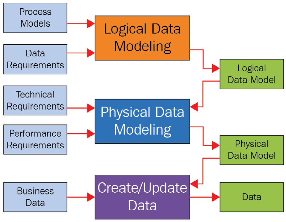
Figure 5.2 – Data modeling approaches

Fun fact

The Enigma machine was used by the German military as the primary mode of communication for all secure wireless communications during World War II. Alan Turing cracked the Enigma code roughly 80 years ago when he figured out the text that's placed at the end of every message. This helped to decipher key secret messages from the German military and helped end the world war. Additionally, this mechanism led to the era of unlocking insights by defining a language to decipher data, which was later formalized as data modeling.

The most common data modeling technique for a database is an Entity-Relationship (ER) model. An ER model in software engineering is a common way to represent the relationship between different entities such as people, objects, places, events, and more in a graphical way in order to organize information better to drive the business processes of an organization. In other terms, an ER model is an abstract data model that defines a data structure for the required information and can be independent of any specific database technology. In this section, we will explain the different data models using the ER model approach. First, let's define, with the help of a use case diagram, the relationship between a customer and their devices associated with a connected HBS hub:

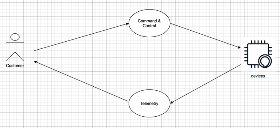
Figure 5.3 – A use case diagram

Now, let's build the ER diagram through a series of conceptual, logical, and physical models:

1. The conceptual data model defines the entities and their relationships. This is the first step of the data modeling exercise and is used by personas such as data architects to gather the initial set of requirements from the business stakeholders. For example, sensor, device, and customer are three entities in a relationship, as shown in the following diagram:
   

   Figure 5.4 – A conceptual data model

2. The conceptual model is then rendered into a logical data model. In this step of data modeling, the data structure along with additional properties are defined using a conceptual model as the foundation.

   For example, you can define the properties of the different entities in the relationship such as the sensor type or device identifier (generally, a serial number or a MAC address), as shown in the following list. Additionally, there could be different forms of relationships, such as the following:

   • Association is the relationship between devices and sensors.
   • Ownership is the relationship between customers and devices.

   The preceding points are illustrated in the following diagram:

   

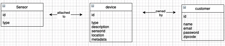
   Figure 5.5 – A logical data model

3. The final step in data modeling is to build a physical data model from the defined logical model. A physical model is often a technology or product-specific implementation of the data model. For example, you define the data types for the different properties of an entity, such as a number or a string, that will be deployed on a database solution from a specific vendor:

Figure 5.6 – A physical data model

Enterprises have used ER modeling for decades to design and govern complex distributed data solutions. All the preceding steps can be visualized as the following workflow, which is not limited to any specific technology, product, subject area, or operating environment (such as a data center, cloud, or edge):

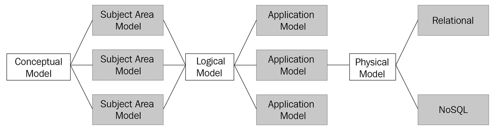
Figure 5.7 – The data modeling flow

Now that you have understood the foundations of data modeling, in the next section, let's examine how this can be achieved for IoT workloads.

How do you design data models for IoT?

Now, let's take a look at some examples of how to apply the preceding data modeling concepts to the realm of structured, unstructured, and semi-structured data that are common with IoT workloads. Generally, when we refer to data modeling for structured data, a relational database (RDBMS) comes to mind first. However, for most IoT workloads, structured data generally includes hierarchical relationships between a device and other entities. And that is better illustrated using a graph or an ordered key-value database. Similarly, for semi-structured data, when it comes to IoT workloads, it's mostly illustrated as a key-value, time series, or document store.  

In this section, we will give you a glimpse of data modeling techniques using NoSQL data solutions to continue building additional functionalities for HBS. Modeling an RDBMS is outside the scope of this book. However, if you are interested in learning about them, there are tons of materials available on the internet that you can refer to.

NoSQL databases are designed to offer freedom to developers to break away from a longer cycle of database schema designs. However, it's a mistake to assume that NoSQL databases lack any sort of data model. Designing a NoSQL solution is quite different from an RDBMS design. For RDBMS, developers generally create a data model that adheres to normalization guidelines, without focusing on access patterns. The data model can be modified later when new business requirements arise, thus leading to a lengthy release cycle. The collected data is organized in different tables with rows, columns, and referential integrities. In contrast, for a NoSQL solution design, developers cannot begin designing the models until they know the questions that are required to be answered. Understanding the business queries working backward from the use case is quintessential. Therefore, the general rule of thumb to remember during data modeling through a relational or NoSQL database is the following:

• Relational modeling primarily cares about the structure of data. The design principle is What answers do I get? 
• NoSQL modeling primarily cares about application-specific access patterns. The design principle is What questions do I ask? 

  Fun fact

  The common translation of the NoSQL acronym is Not only SQL. This highlights the fact that NoSQL doesn't only support NoSQL, but it can handle relational, semi-structured, and unstructured data. Organizations such as Amazon, Facebook, Twitter, LinkedIn, and Google have designed different NoSQL technologies.

Before I show you some examples of data modeling, let's understand the five fundamental properties of our application's (that is, the HBS hub) access patterns that need to be considered in order to come up with relevant questions:

• Data type: What's the type of data in scope? For example, is the data related to telemetry, command-control, or critical events? Let's quickly refresh the use of each of these data types:

  a) Telemetry: This is a constant stream of data transmitted by sensors/actuators, such as temperature or humidity readings , which can be aggregated on the edge or published as it is to the cloud for further processing.

  b) Command and Control: These are actionable messages, such as turning on/off the lights, which can occur between two devices or between an end user and the device.

  c) Events: These are data patterns that identify more complex scenarios than regular telemetry data, such as network outages in a home or a fire alarm in a building.

• Data size: What is the quantity of data in scope? Is it necessary to store and retrieve data locally (on the edge), or does the data require transmission to a different data persistence layer (such as a data lake on the cloud)?
• Data shape: What's the form of data being generated from different edge devices such as text, blobs, and images? Note that different data forms such as images and videos might have different computational needs (think of GPUs).
• Data velocity: What's the speed of data to process queries based on the required latencies? Do you have a hot, warm, or cold path of data?
• Data consistency: How much of this data needs to have strong versus eventual consistency?

Answering the preceding questions will help you to determine whether the solution should be based on one of the following:

• BASE methodology: Basically Available, Soft-state, Eventual consistency, which are typical characteristics of NoSQL databases
• ACID methodology: Atomicity, Consistency, Isolation, and Durability, which are typical characteristics of relational databases

We will discuss these concepts in more detail next.

Selecting between ACID or BASE for IoT workloads

The following table lists some of the key differences between the two methodologies. This should enable you to make an informed decision working backward from your use case:

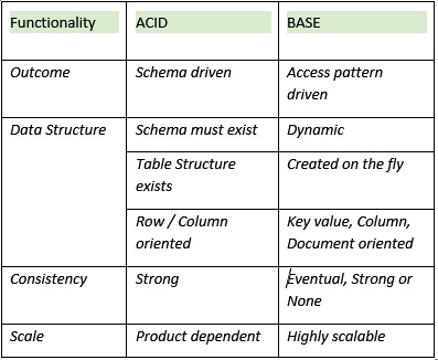
Figure 5.8 – ACID versus BASE summary

Fun fact

ACID and BASE represent opposing sides of the pH spectrum. Jim Grey conceived the idea in 1970 and subsequently published a paper, called The Transaction Concept: Virtues and Limitations, in June 1981.

So far, you have understood the fundamentals of data modeling and design approaches. You must be curious about how to relate those concepts to the connected HBS product, which you have been developing in earlier chapters. Let's explore how the rubber meets the road.

Do you still remember the first phase of data modeling?

Bingo! Conceptual it is.

Conceptual modeling of the connected HBS hub

The following diagram is a hypothetical conceptual model of the HBS hub:

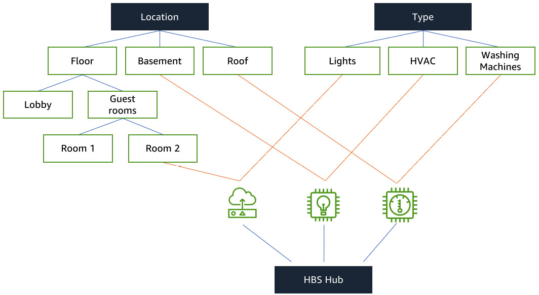
Figure 5.9 – A conceptual data model for connected HBS

In the preceding diagram, you can observe how the different devices such as lights, HVAC, and washing machines are installed in different rooms of a house. Now the conceptual model is in place, let's take a look at the logical view.

The logical modeling of the connected HBS hub

To build the logical model, we need to ask ourselves the type of questions an end consumer might ask, such as the following:

• Show the status of a device (such as is the washing complete?).
• Turn a device on or off (such as turn off the lights).
• Show the readings of a device (such as what's the temperature now?).
• Take a new reading (such as how much energy is being consumed by the refrigerator?).
• Show the aggregated connectivity status of a device (or devices) for a period.

To address these questions, let's determine the access patterns for our end application:

Figure 5.10 – A logical data model for connected HBS

Now that we have captured the summary of our data modeling requirements, you can observe that the solution needs to ingest data in both structured and semi-structured formats at high frequency. Additionally, it doesn't require strong consistency. Therefore, it makes sense to design the data layer using a NoSQL solution that leverages the BASE methodology.

The physical modeling of the connected HBS hub

As the final step, we need to define the physical data model from the gathered requirements. To do that, we will define a primary and a secondary key. You are not required to define all of the attributes if they're not known to you, which is a key advantage of a NoSQL solution.

Defining the primary key

As the name suggests, this is one of the required attributes in a table, which is often known as a Partition key. In a table, no two primary keys should have the same value. There is also a concept of a Composite key. It's composed of two attributes, a partition key and a Sort key.

In our scenario, we will create a Sensor table with a composite key (as depicted in the following screenshot). The primary key is a device identifier, and the sort key is a timestamp that enables us to query data in a time range:

Figure 5.11 – Composite keys in a sensor table

Defining the secondary indexes

A secondary index allows us to query the data in the table using a different key, in addition to queries against the primary or composite keys. This gives your applications more flexibility in querying the data for different use cases. Performing a query using a secondary index is pretty similar to querying from the table directly.

Therefore, for secondary indexes, as shown in the following chart, we have selected the primary key as a sensor identifier (sensor_id) along with timestamp as the sort key:

Figure 5.12 – Secondary indexes in a sensor table

Defining the additional attributes

The key advantage of a NoSQL solution is that there is no enforced schema. Therefore, other attributes can be created on the fly as data comes in. That being said, if some of the attributes are already known to the developer, there is no restriction to include those in the data model:

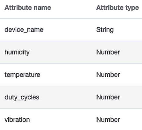
Figure 5.13 – Other attributes in a sensor table

Now that the data layer exists, let's create the interfaces to access this data.

Defining the interfaces

Now we will create two different facets for the sensor table. A facet is a virtual construct that enables different views of the data stored in a table. The facets can be mapped to a functional construct such as a method or an API for performing various Create, Read, Update, Delete (CRUD) operations on a table:

• putItems: This facet allows write operations and requires the composite keys at the minimum in the payload.
• getItems: This facet allows read operations that can query items with all or selective attributes.

The following screenshot depicts the getItems facet definition:

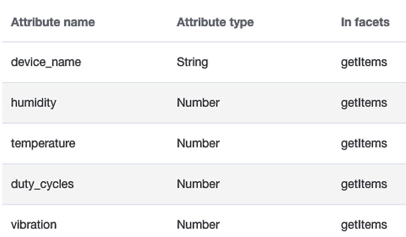
Figure 5.14 – The getItems facet definition

So, now you have created the data model along with its interfaces. This enables you to understand the data characteristics that are required to develop edge applications.

Designing data patterns on the edge

As data flows securely from different sensors/actuators on the edge to the gateway or cloud over different protocols or channels, it is necessary for it to be safely stored, processed, and cataloged for further consumption. Therefore, any IoT data architecture needs to take into consideration the data models (as explained earlier), data storage, data flow patterns, and anti-patterns, which will be covered in this section. Let's start with data storage.

Data storage

Big data solutions on the cloud are designed to reliably store terabytes, petabytes, or exabytes of data and can scale across multiple geographic locations globally to provide high availability and redundancy for businesses to meet their Recovery Time Objective (RTO) and Recovery Point Objective (RPO). However, edge solutions, such as our very own connected HBS hub solution, are resource-constrained in terms of compute, storage, and network. Therefore, we need to design the edge solution to cater to different time-sensitive, low-latency use cases and hand off the heavy lifting to the cloud. A data lake is a well-known pattern on the cloud today, which allows a centralized repository to store data as it arrives, without having to first structure the data. Thereafter, different types of analytics, machine learning, and visualizations can be performed on that data for consumers to achieve better business outcomes. So, what is the equivalent of a data lake for the edge?

Let's introduce a new pattern, called a data pond, for the authoritative source of data (that is, the golden source) that is generated and temporarily persisted on the edge. Certain characteristics of a data pond are listed as follows:

• A data pond enables the quick ingestion and consumption of data in a fast and flexible fashion. A data producer is only required to know where to push the data, that is, the local storage, local stream, or cloud. The choice of the storage layer, schema, ingestion frequency, and quality of the data is left to the data producer.
• A data pond should work with low-cost storage. Generally, IoT devices are low in storage; therefore, only highly valuable data that's relevant for the edge operations can be persisted locally. The rest of the data is pushed to the cloud for additional processing or thrown away (if noisy).
• A data pond supports schema on read. There can be multiple streams supporting multiple schemas in a data pond.
• A data pond should support the data protection mechanisms at rest and in encryption. It's also useful to implement role-based access that allows auditing the data trail as it flows from the edge to the cloud.

The following diagram shows an edge architecture of how data collected from different sensors/actuators can be persisted and securely governed in a data pond:

Figure 5.15 – A data pond architecture at the edge

The organizational entities involved in the preceding data flow include the following:

• Data producers: These are entities that generate data. These include physical (such as sensors, actuators, or associated devices) or logical (such as applications) entities and are configured to store data in the data pond or publish data to the cloud.
• Data pond team: Generally, the data operations team defines the data access mechanisms for the data pond (or lake) and the development team supports data management.
• Data consumers: Edge and cloud applications retrieve data from the data pond (or lake) using the mechanisms authorized to further iterate on the data and meet business needs.

The following screenshot shows the organizational entities for the data pond:

Figure 5.16 – The organizational entities for the data pond

Now you have understood how data can be stored on a data pond and be managed or governed by different entities. Next, let's discuss the different flavors of data and how they can be integrated.

Data integration concepts

DII occurs through different layers, as follows:

• Batch: This layer aggregates data that has been generated by data producers. The goal is to increase the accuracy of data insights through the consolidation of data from multiple sources or dimensions.
• Speed: This layer streams data generated by data producers. The goal is to allow a near real-time analysis of data with an acceptable level of accuracy.
• Serving: This layer merges the data from the batch layer and the speed layer to enable the downstream consumers or business users with holistic and incremental insights into the business.

The following diagram is an illustration of DII:

Figure 5.17 -- Data Integration and Interoperability (DII)

As you can see, there are multiple layers within the data flow that are commonly implemented using the Extract, Transform, and Load (ETL) methodology or the Extract, Load, and Transform (ELT) methodology in the big data world. The ETL methodology involves steps to extract data from different sources, implement data quality and consistency standards, transform (or aggregate) the data to conform to a standard format, and load (or deliver) data to downstream applications.

The ELT process is a variant of ETL with similar steps. The difference is that extracted data is loaded before the transformation. This is common for edge workloads as well, where the local gateway might not have enough resources to do the transformation locally; therefore, it publishes the data prior to additional processing.

But how are these data integration patterns used in the edge? Let's explore this next.

Data flow patterns

An ETL flow on the edge will include three distinct steps, as follows:

1. Data extraction from devices such as sensors/actuators
2. Data transformation to clean, filter, or restructure data into an optimized format for further consumption
3. Data loading to publish data to the persistence layer such as a data pond, a data lake, or a data warehouse

For an ELT flow, steps 2 and 3 will take place in the reverse order.

An ETL Scenario for a Connected Home

For example, in a connected home scenario, it's common to extract data from different sensors/actuators, followed by a data transformation that might include format changes, structural changes, semantic conversions, or deduplication. Additionally, data transformation allows you to filter out any noisy data from the home (think of a crying baby or a noisy pet), resulting in reduced network charges of publishing all the bits and bytes to the cloud. Based on a use case such as an intrusion alert or replenishing a printer toner, data transformation can be performed in batch or real time, by eitherphysically storing the result in a staging area or virtually storing the transferred data in memory until you are ready to move to the load step.

These core patterns (ETL or ELT) have evolved, with time, into different data flow architectures, such as event-driven, batch, lambda, and complex event processing (CEP). We will explain each of them in the next section.

Event-driven (or streaming)

It's very common for edge applications to generate and process data in smaller sets throughout the day when an event happens. Near real-time data processing has a lower latency and can be both synchronous and asynchronous.

In an asynchronous data flow, the devices (such as sensors) do not wait for the receiving system to acknowledge updates before continuing processing. For example, in a connected home, a motion/occupancy sensor can trigger an intruder notification based on a detected event but continue to monitor without waiting for an acknowledgment.

In comparison, in a real-time synchronous data flow, no time delay or other differences between source and target are acceptable. For example, in a connected home, if there is a fire alarm, it should notify the emergency services in a deterministic way.

With AWS Greengrass, you can design both synchronous and asynchronous data communications. In addition to this, as we build multi-faceted architectures on the edge, it's quite normal to build multiprocessing or multithreaded polyglot solutions on the edge to support different low-latency use cases:

Figure 5.18 – Event-driven architecture at the edge

Micro-batch (or aggregated processing)

Most enterprises perform frequent batch processing to enable end users with business insights. In this mode, data moving will represent either the full set of data at a given point in time, such as the energy meter reading of a connected home at the end of a period (such as the day, week, or month), or data that has changed values since the last time it was sent, such as a hvac reading or a triggered fire alarm. Generally, batch systems are designed to scale and grow proportionally along with the data. However, that's not feasible on the edge due to the lack of horsepower, as explained earlier.

Therefore, for IoT use cases, leveraging micro-batch processing is more common. Here, the data is stored locally and is processed on a much higher frequency, such as every few seconds, minutes, hours, or days (over weeks or months). This allows data consumers to gather insights from local data sources with reduced latency and cost, even when disconnected from the internet. The Stream Manager capability of AWS Greengrass allows you to perform aggregated processing on the edge. Stream Manager brings enhanced functionalities regarding how to process data on the edge such as defining a bandwidth and data prioritization for multiple channels, timeout behavior, and direct export mechanisms to different AWS services such as Amazon S3, AWS IoT Analytics, AWS IoT SiteWise, and Amazon Kinesis data streams:

Figure 5.19 – Micro-batch architecture at the edge

Lambda architecture

Lambda architecture is an approach that combines both micro-batch and stream (near real-time) data processing. It makes the consolidated data available for downstream consumption. For example, a refrigeration unit, a humidifier, or any critical piece of machinery on a manufacturing plant can be monitored and fixed before it becomes non-operational. So, for a connected HBS hub solution, micro-batch processing will allow you to detect long-term trends or failure patterns. This capability in turn, will help your fleet operators recommend preventive or predictive maintenance for the machines to end consumers. This workflow is often referred to as the warm or cold path of the data analytics flow.

On the other hand, stream processing will allow the fleet operators to derive near real-time insights through telemetry data. This will enable consumers to take mission-critical actions such as locking the entire house and calling emergency services if any theft is detected. This is also referred to as the hot path in lambda architecture:

Figure 5.20 – Lambda architecture at the edge

Fun fact

Lambda architecture has nothing to do with the AWS lambda service. The term was coined by Nathan Marz, who worked on big-data-related technologies at BackType and Twitter. This is a design pattern for describing data processing that is scalable and fault-tolerant.

Data flow anti-patterns for the edge

So far, we have learned about the common data flow patterns on the edge. Let's also discuss some of the anti-patterns.

Complex Event Processing (CEP)

Events are data patterns that identify complex circumstances from ingested data, such as network outages in a home or a fire alarm in a building. It might be easier to detect events from a few sensors or devices; however, getting visibility into complex events from disparate sources and being able to capture states or trigger conditional logic to identify and resolve issues quickly requires special treatment.

That's where the CEP pattern comes into play. CEP can be resource-intensive and needs to scale to all sizes of data and grow proportionally. Therefore, it's still not a very common pattern on the edge. On the cloud, managed services such as AWS IoT events or AWS EventBridge can make it easier for you to perform CEP on the data generated from your IoT devices.

Batch

Traditionally, in batch processing, data moves in aggregates as blobs or files either on an ad hoc request from a consumer or automatically on a periodic schedule. Data will either be a full set (referred to as snapshot) or a changed set (delta) from a given point in time. Batch processing requires continuous scaling of the underlying infrastructure to facilitate the data growth and processing requirements. Therefore, it's a pattern that is better suited for big data or data warehousing solutions on the cloud. That being said, for an edge use case, you can still leverage the micro-batch pattern (as explained earlier) to aggregate data that's feasible in the context of a resource-constrained environment.

Replication

It's a common practice on the cloud to maintain redundant copies of datasets across different locations to improve business continuity, improve the end user experience, or enhance data resiliency. However, in the context of the edge, data replication can be expensive, as you might require redundant deployments. For example, with a connected HBS hub solution, if the gateway needs to support redundant storage for replication, it will increase the bill of materials (BOM) cost of the hardware, and you can lose the competitive edge on the market.

Archiving

Data that is used infrequently or not actively used can be moved to an alternate data storage solution that is more cost-effective to the organization. Similar to replication, for archiving data locally on the edge, additional deployment of hardware resource is necessary. This increases the bill of materials (BOM) cost of the device and leads to additional operational overhead. Therefore, it's common to archive the transformed data from the data lake to a cost-effective storage service on the cloud such as Amazon Glacier. Thereafter, this data can be used for local operations, data recovery, or regulatory needs.

A hands-on approach with the lab

In this section, you will learn how to build a lambda architecture on the edge using different AWS services. The following diagram shows the lambda architecture:

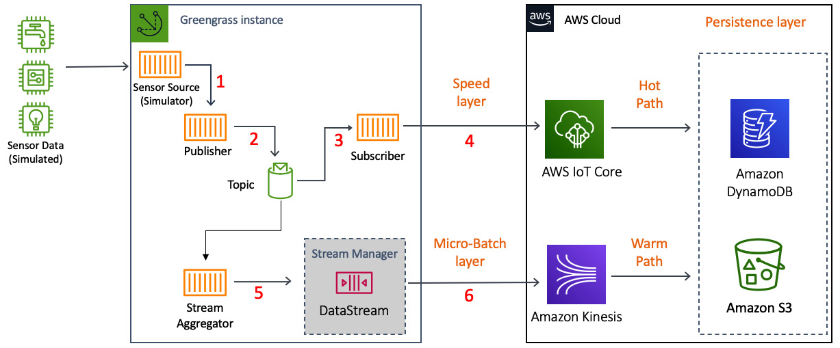
Figure 5.21 – The lab architecture

The preceding workflow uses the following services. In this chapter, you will complete steps 1–6 (as shown in Figure 5.21). This includes designing and deploying the edge components, processing, and transforming data locally, and pushing the data to different cloud services:

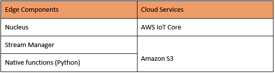
Figure 5.22 – The hands-on lab components

In this hands-on section, your objective will consist of the following:

1. Build the cloud resource (that is, Amazon Kinesis data streams, Amazon S3 bucket, and DynamoDB tables).
2. Build and deploy the edge components (that is, artifacts and recipes) locally on Raspberry Pi.
3. Validate that the data is streamed from the edge to the cloud (AWS IoT Core).

Building cloud resources

Deploy the CloudFormation template from the chapter5/cfn folder to create cloud resources such as Amazon S3 buckets, Kinesis data streams, and DynamoDB tables. You will need to substitute these respective names from the Resources section of the deployed stack, when requested, in the following section.

Building edge components

Now, let's hop on to our device to build and deploy the required edge components:

1. Navigate to the following working directory from the Terminal of your Raspberry Pi device:

   cd hbshub/artifacts

2. Open the Python script using the editor of your choice (such as nano, vi, or emac):

   nano com.hbs.hub.Publisher/1.0.0/hbs_sensor.py

   The following code simulates data from the fictional sensors associated with the HBS hub. In the real world, data will be published from the real sensors over serial or GPIO, which needs to be captured. The following function is in a DummySensor class that will be referenced by the Publisher component in the next step:

       def read_value(self):

           message = {}

           

           device_list = ['hvac', 'refrigerator', 'washingmachine']

           device_name = random.choice(device_list)

           

           if device_name == 'hvac' :

               message['device_id'] = "1"

               message['timestamp'] = float("%.4f" % (time()))

               message['device_name'] = device_name

               message['temperature'] = round(random.uniform(10.0, 99.0), 2)

               message['humidity'] = round(random.uniform(10.0, 99.0), 2)

           elif device_name == 'washingmachine' :

               message['device_id'] = "2"

               message['timestamp'] = float("%.4f" % (time()))

               message['device_name'] = device_name

               message['duty_cycles'] = round(random.uniform(10.0, 99.0), 2)

           else :

               message['device_id'] = "3"

               message['timestamp'] = float("%.4f" % (time()))

               message['device_name'] = device_name

               message['vibration'] = round(random.uniform(100.0, 999.0), 2)

           

           return message

3. Now, open the following publisher script and navigate through the code:

   nano com.hbs.hub.Publisher /1.0.0/hbs_publisher.py

   The following publisher code streams the data from the dummy sensors, as explained in the previous step, to a hbs/localtopic topic every 10 seconds over ipc:

   TIMEOUT = 10

   ipc_client = awsiot.greengrasscoreipc.connect()

   sensor = DummySensor()

   while True:

       message = sensor.read_value()

       message_json = json.dumps(message).encode('utf-8')

       request = PublishToTopicRequest()

       request.topic = args.pub_topic

       publish_message = PublishMessage()

       publish_message.json_message = JsonMessage()

       publish_message.json_message.message = message

       request.publish_message = publish_message

       operation = ipc_client.new_publish_to_topic()

       operation.activate(request)

       future = operation.get_response()

       future.result(TIMEOUT)

       print("publish")

       time.sleep(5)

4. Now you have reviewed the code, check the following recipe file to review the access controls and dependencies that are required by the Publisher component:

   cd ~/hbshub/recipes

   nano com.hbs.hub.Publisher-1.0.0.yaml

5. Now we have the component and the recipe, let's create a local deployment:

   sudo /greengrass/v2/bin/greengrass-cli deployment create   --recipeDir ~/hbshub/recipes --artifactDir ~/hbshub/artifacts --merge "com.hbs.hub.Publisher=1.0.0"

   Local deployment submitted! Deployment Id: xxxxxxxxxxxxxx

6. Verify that the component has successfully been deployed (and is running) using the following command:

   sudo /greengrass/v2/bin/greengrass-cli component list

   The following is the output:

   Components currently running in Greengrass:

   Component Name: com.hbs.hub.Publisher

       Version: 1.0.0

       State: RUNNING

7. Now that the Publisher component is up and running, let's review the code in the Subscriber component as well:

   cd hbshub/artifacts

   nano com.hbs.hub.Subscriber/1.0.0/hbs_subscriber.py

   The Subscriber component subscribes to the hbs/localtopic topic over the ipc protocol and gets triggered by the published events from the publisher:

   def setup_subscription():

       request = SubscribeToTopicRequest()

       request.topic = args.sub_topic

       handler = StreamHandler()

       operation = ipc_client.new_subscribe_to_topic(handler)

       future = operation.activate(request)

       future.result(TIMEOUT)

       return operation

   Then, the subscriber pushes the messages over mqtt to the hbs/cloudtopic cloud topic on AWS IoT Core:

   def send_cloud(message_json):

       message_json_string = json.dumps(message_json)

       request = PublishToIoTCoreRequest()

       request.topic_name = args.pub_topic

       request.qos = QOS.AT_LEAST_ONCE

       request.payload = bytes(message_json_string,"utf-8")

       publish_message = PublishMessage()

       publish_message.json_message = JsonMessage()

       publish_message.json_message.message = bytes(message_json_string, "utf-8")

       request.publish_message = publish_message

       operation = ipc_client.new_publish_to_iot_core()

       operation.activate(request)

       logger.debug(message_json)

8. Now you have reviewed the code, let's check the following recipe file to review the access controls and dependencies required by the Subscriber component:

   cd ~/hbshub/recipes

   nano com.hbs.hub.Subscriber-1.0.0.yaml

9. Now we have the component and the recipe, let's create a local deployment:

   sudo /greengrass/v2/bin/greengrass-cli deployment create   --recipeDir ~/hbshub/recipes --artifactDir ~/hbshub/artifacts --merge "com.hbs.hub.Subscriber=1.0.0"

   The following is the output:

   Local deployment submitted! Deployment Id: xxxxxxxxxxxxxx

10. Verify that the component has successfully been deployed (and is running) using the following command. Now you should see both the Publisher and Subscriber components running locally:

    sudo /greengrass/v2/bin/greengrass-cli component list

    The following is the output:

    Components currently running in Greengrass:

    Component Name: com.hbs.hub.Publisher

        Version: 1.0.0

        State: RUNNING

    Component Name: com.hbs.hub.Subscriber

        Version: 1.0.0

        State: RUNNING

11. As you have observed, in the preceding code, the Subscriber component will not only subscribe to the local mqtt topics on the Raspberry Pi, but it will also start publishing data to AWS IoT Core (on the cloud). Let's verify that from the AWS IoT console:

    Please navigate to AWS IoT console. | Select Test (on the left pane). | Choose MQTT Client. | Subscribe to Topics. | Type hbs/cloudtopic. | Click Subscribe.

    Tip

    If you have changed the default topic names in the recipe file, please use that name when you subscribe; otherwise, you won't see the incoming messages.

12. Now that you have near real-time data flowing from the edge to the cloud, let's work on the micro-batch flow by integrating with Stream Manager. This component will subscribe to the hbslocal/topic topic (same as the subscriber). However, it will append the data to a local data stream using the Stream Manager functionality rather than publishing it to the cloud. Stream Manager is a key functionality for you to build a lambda architecture on the edge. We will break down the code into different snippets for you to understand these concepts better. So, let's navigate to the working directory:

    nano com.hbs.hub.Aggregator/1.0.0/hbs_aggregator.py

13. First, we create a local stream with the required properties such as stream name, data size, time to live, persistence, data flushing, data retention strategy, and more. Data within the stream can stay local for further processing or can be exported to the cloud using the export definition parameter. In our case, we are exporting the data to Kinesis, but you can use a similar approach to export the data to other supported services such as S3, IoT Analytics, and more:

    iotclient.create_message_stream(

         MessageStreamDefinition(

           name=stream_name,  

           max_size=268435456,  

           stream_segment_size=16777216,  

           time_to_live_millis=None,

         strategy_on_full=StrategyOnFull.OverwriteOldestData,  

           persistence=Persistence.File,  

           flush_on_write=False,  

           export_definition=ExportDefinition(

                kinesis=[

                  KinesisConfig(

                      identifier="KinesisExport",

                      kinesis_stream_name=kinesis_stream,

                      batch_size=1,

                      batch_interval_millis=60000,

                      priority=1

14. Now the stream is defined, the data is appended through append_message api:

    sequence_number = client.append_message(stream_name=stream_name, data= event.json_message.message)

    Fact Check

    Stream Manager allows you to deploy a lambda architecture on the edge without having to deploy and manage a separate lightweight database or streaming solution. Therefore, you can reduce the operational overhead or BOM cost of this solution. In addition to this, with Stream Manager as a data pond, you can persist data on the edge using a schema-less approach dynamically (remember BASE?). And finally, you can publish data to the cloud using the native integrations between the Stream Manager and cloud data services, such as IoT Analytics, S3, and Kinesis, without having to write any additional code. Stream Manager can also be beneficial for use cases with larger payloads such as blobs, images, or videos that can be easily transmitted over HTTPS.

15. Now that you have reviewed the code, let's add the required permission for the Stream Manager component to update the Kinesis stream:

    Please navigate to AWS IoT console. | Select Secure (on the left pane). | Choose Role Aliases and select the appropriate one. | Click on the Edit IAM Role. | Attach policies. | Choose Amazon Kinesis Full Access. | Attach policy.

    Please note that it's not recommended to use a blanket policy similar to this for production workloads. This is used here in order to ease the reader into operating in a test environment.

16. Let's perform a quick check of the recipe file prior to deploying this component:

    cd ~/hbshub/recipes

    nano com.hbs.hub.Aggregator-1.0.0.yaml

    Please note the Configuration section in this recipe file, as it requires the Kinesis stream name to be updated. This can be retrieved from the resources section of the deployed CloudFormation stack. Also, note the dependencies on the Stream Manager component and the reference to sdk, which is required by the component at runtime:

    ComponentConfiguration:

      DefaultConfiguration:

        sub_topic: "hbs/localtopic"

        kinesis_stream: "<replace-with-kinesis-stream-from cfn>"

        accessControl:

          aws.greengrass.ipc.pubsub:

            com.hbs.hub.Aggregator:pubsub:1:

              policyDescription: "Allows access to subscribe to topics"

              operations:

                - aws.greengrass#SubscribeToTopic

                - aws.greengrass#PublishToTopic

              resources:

                - "*"

    ComponentDependencies:

      aws.greengrass.StreamManager:

        VersionRequirement: "^2.0.0"

    Manifests:

      - Platform:

          os: all

        Lifecycle:

          Install:

            pip3 install awsiotsdk numpy -t .

          Run: |

            export PYTHONPATH=$PYTHONPATH:{artifacts:path}/stream_manager

            PYTHONPATH=$PWD python3 -u {artifacts:path}/hbs_aggregator.py --sub-topic="{configuration:/sub_topic}" --kinesis-stream="{configuration:/kinesis_stream}"

17. Next, as we have the artifact and the recipe reviewed, let's create a local deployment:

    sudo /greengrass/v2/bin/greengrass-cli deployment create   --recipeDir ~/hbshub/recipes --artifactDir ~/hbshub/artifacts --merge "com.hbs.hub.Aggregator=1.0.0"

    Local deployment submitted! Deployment Id: xxxxxxxxxxxxxx

18. Verify that the component has been successfully deployed (and is running) using the following command. You should observe all the following components running locally:

    sudo /greengrass/v2/bin/greengrass-cli component list

    The output is as follows:

    Components currently running in Greengrass:

    Component Name: com.hbs.hub.Publisher

        Version: 1.0.0

        State: RUNNING

    Component Name: com.hbs.hub.Subscriber

        Version: 1.0.0

        State: RUNNING

    Component Name: com.hbs.hub.Aggregator

        Version: 1.0.0

        State: RUNNING

19. The Aggregator component will publish the data directly from the local stream to the Kinesis stream on the cloud. Let's navigate to the AWS S3 console to check whether the incoming messages are appearing:

    Go to the Amazon Kinesis console. | Select Data Streams. | Choose the stream. | Go to the Monitoring tab. | Check the metrics such as Incoming data or Get records.

If you see the metrics showing some data points on the chart, it means the data is successfully reaching the cloud.

Note

You can always find the specific resource names required for this lab (such as the preceding Kinesis stream) in the Resources or Output section of the CloudFormation stack deployed earlier.

Validating the data streamed from the edge to the cloud

In this section, you will perform some final validation to ensure the transactional and batch data streamed from the edge components is successfully persisted on the data lake:

1. In step 19 of the previous section, you validated that the Kinesis stream is getting data through metrics. Now, let's understand how that data is persisted to the data lake from the streaming layer:

   Go to the Amazon Kinesis console. | Select Delivery Streams. | Choose the respective delivery stream. | Click on the Configuration tab. | Scroll down to Destination Settings. | Click on the S3 bucket under the Amazon S3 destination.

   Click on the bucket and drill down to the child buckets that store the batch data in a zipped format to help optimize storage costs.

2. As the final step, navigate to AWS DynamoDB to review the raw sensor data streaming in near real time through AWS IoT Core:

   On the DynamoDB console, choose Tables. Then, select the table for this lab. Click on View Items.

   Can you view the time series data? Excellent work.

   Note

   If you are not able to complete any of the preceding steps, please refer to the Troubleshooting section in the GitHub repository or create an issue for additional instructions.

Congratulations! You have come a long way to learn how to build a lambda architecture that spans from the edge to the cloud using different AWS edge and cloud services. Now, let's wrap up with some additional topics before we conclude this chapter.

Additional topics for reference

Aside from what we have read so far, there are a couple of topics that I wish to mention. Whenever you have the time, please check them out, as they do have lots of benefits and can be found online.

Time series databases

In this chapter, we learned how to leverage a NoSQL (key-value) data store such as Amazon DynamoDB for persisting time series data. Another common way to persist IoT data is to use a time series database (TSDB) such as Amazon Timestream or Apache Cassandra. As you know by now, time series data consists of measurements or events collected from different sources such as sensors and actuators that are indexed over time. Therefore, the fundamentals of modeling a time series database are quite similar to what was explained earlier with NoSQL data solutions. So, the obvious question that remains is How do you choose between NoSQL and TSDB? Take a look at the following considerations:

• Consider the data summarization and data precision requirements:

  For example, show me the energy utilization on a monthly or yearly basis. This requires going over a series of data points indexed by a time range to calculate a percentile increase of energy over the same period in the last 12 weeks, summarized by weeks. This kind of querying could get expensive with a distributed key-value store.

• Consider purging the data after a period of time:

  For example, do consumers really care about the high precision metrics from an hourly basis to calculate their overall energy utilization per month? Probably not. Therefore, it's more efficient to store high-precision data for a short period of time and, thereafter, aggregated and downsampled data for identifying long-term trends. This functionality can partially be achieved with some NoSQL databases as well (such as the DynamoDB item expiry functionality). However, TSDBs are better suited as they can also offer downsampling and aggregation capabilities using different means, such as materialized views.

Unstructured data

You must be curious that most of our discussion in this chapter was related to structured and semi-structured data. We did not touch upon unstructured data (such as images, audio, and videos) at all. You are spot on. Considering IoT is the bridge between the physical world and the cyber world, there will be a huge amount of unstructured data that will need to be processed for different analytics and machine learning use cases.

For example, consider a scenario where the security cameras installed in your customer's home detect any infiltration or unexpected movements through the motion sensors and start streaming a video feed of the surroundings. The feed will be available through your smart hub or mobile devices for consumption. Therefore, in this scenario, the security camera is streaming videos that are unstructured data, as a P2P feed that can also be stored (if the user allows) locally on the hub or to an object store on the cloud. In Chapter 7, Machine Learning Workloads at the Edge, you will learn the techniques to ingest, store, and infer unstructured data from the edge. However, we will not delve into the modeling techniques for unstructured data, as it primarily falls under data science and is not very relevant in the day-to-day life of IoT practitioners.

Summary

In this chapter, you learned about different data modeling techniques, data storage, and data integration patterns that are common with IoT edge workloads. You learned how to build, test, and deploy edge components on Greengrass. Additionally, you implemented a lambda architecture to collect, process, and stream data from disparate sources on the edge. Finally, you validated the workflow by visualizing the incoming data on IoT Core.

In the next chapter, you will learn how all this data can be served on the cloud to generate valuable insights for different end consumers.

Knowledge check

Before moving on to the next chapter, test your knowledge by answering these questions. The answers can be found at the end of the book: 

1. True or false: Data modeling is only applicable for relational databases.
2. What is the benefit of performing a data modeling exercise?
3. Is there any relevance of ETL architectures for edge computing? (Hint: Think lambda.)
4. True or false: Lambda architecture is the same as AWS lambda service.
5. Can you think of at least one benefit of data processing at the edge?
6. Which component of Greengrass is required to be run at the bare minimum for the device to be functional?
7. True or false: Managing streams for real-time processing is a cloud-only thing.
8. What strategy could you implement to persist data on the edge locally for a longer time?

References

Take a look at the following resources for additional information on the concepts discussed in this chapter:

• Data Management Body of Knowledge: https://www.dama.org/cpages/body-of-knowledge
• Amazon's Dynamo: https://www.allthingsdistributed.com/2007/10/amazons_dynamo.html
• NoSQL Design for DynamoDB: https://docs.aws.amazon.com/amazondynamodb/latest/developerguide/bp-general-nosql-design.html
• Lambda Architecture: http://lambda-architecture.net/
• Managing data streams on the AWS IoT Greengrass Core: https://docs.aws.amazon.com/greengrass/v2/developerguide/manage-data-streams.html
• Data Lake on AWS: https://aws.amazon.com/solutions/implementations/data-lake-solution/