Chapter 6: Processing and Consuming Data on the Cloud

The value proposition of edge computing is to process data closer to the source and deliver intelligent near real-time responsiveness for different kinds of applications across different use cases. Additionally, edge computing reduces the amount of data that is required to be transferred to the cloud, thus saving on network bandwidth costs. Often, high-performance edge applications require local compute, local storage, network, data analytics, and machine learning capabilities to process high-fidelity data in low latencies. Although AWS IoT Greengrass allows you to run sophisticated edge applications on devices and gateways, it will be resource-constrained compared to the horsepower from the cloud. Therefore, for different use cases, it's quite common to leverage the scale of cloud computing for high-volume complex data processing needs.

In the previous chapter, you learned about the different design patterns around data transformation strategies on the edge. This chapter will focus on explaining how you can build different data workflows on the cloud based on the data velocity, data variety, and data volume collected from the HBS hub running a Greengrass instance. Specifically, you will learn how to persist data in a transactional data store, develop API driven access, and build a serverless data warehouse to serve data to end users. Therefore, the chapter is divided into the following topics:

• Defining big data for IoT workloads
• Introduction to Domain-Driven Design (DDD) concepts
• Design data flow patterns on the cloud
• Remembering data flow anti-patterns for edge workloads

Technical requirements

The technical requirements for this chapter are the same as those outlined in Chapter 2, Foundations of Edge Workloads. See the full requirements in that chapter.

Defining big data for IoT workloads

The term Big in Big data is relative, as the influx of data has grown substantially in the last two decades from terabytes to exabytes due to the digital transformation of enterprises and connected ecosystems. The advent of big data technologies has allowed people (think social media) and enterprises (think digital transformation) to generate, store, and analyze huge amounts of data. To analyze datasets of this volume, sophisticated computing infrastructure is required that can scale elastically based on the amount of input data and required outcome. This characteristic of big data workloads, along with the availability of cloud computing, democratized the adoption of big data technologies by companies of all sizes. Even with the evolution of edge computing, big data processing on the cloud plays a key role in IoT workloads, as data is more valuable when it's adjacent and enriched with other data systems. In this chapter, we will learn how the big data ecosystem allows for advanced processing and analytical capabilities on the huge volume of raw measurements or events collected from the edge to enable the consumption of actionable information by different personas.

The integration of IoT with big data ecosystems has opened up a diverse set of analytical capabilities that allows the generation of additional business insights. These include the following:

• Descriptive analytics: This type of analytics helps users answer the question of what happened and why? Examples of this include traditional queries and reporting dashboards.
• Predictive analytics: This form of analytics helps users predict the probability of a given event in the future based on historical events or detected anomalies. Examples of this include early fraud detection in banking transactions and preventive maintenance for different systems.
• Prescriptive analytics: This kind of analytics helps users provide specific (clear) recommendations. They address the question of what should I do if x happens? Examples of this include an election campaign to reach out to targeted voters or statistical modeling in wealth management to maximize returns.

The outcome of these processes allows organizations to have increased visibility to new information, emerging trends, or hidden data correlation to improve efficiencies or generate new revenue streams. In this chapter, you will learn about the approaches of both descriptive and predictive analytics on data collected from the edge. In addition to this, you will learn how to implement design patterns such as streaming to a data lake or a transactional data store on the cloud, along with leveraging API driven access, which are considered anti-patterns for the edge. So, let's get started with the design methodologies of big data that are relevant for IoT workloads.

What is big data processing?

Big data processing is generally categorized in terms of the three Vs: the volume of data (for example, a terabyte, petabyte, or more), the variety of data (that is, structured, semi-structured, or unstructured), and the velocity of data (that is, the speed with which it's produced or consumed). However, as more organizations begin to adopt big data technologies, there have been additions to the list of Vs, such as the following:

• Viscosity: This emphasizes the ease of usability of data; for example, there could be noisy data collected from the edge that's not easy to parse.
• Volatility: This refers to how often data changes occur and, therefore, how long the data is useful; for example, capturing specific events at home can be more useful than every other activity.
• Veracity: This refers to how trustworthy the data is, for example, if images captured from outdoor cameras are of poor quality, they cannot be trusted to identify intrusion.

For edge computing and the Internet of Things (IoT), all six Vs are relevant. The following diagram presents a visual summary of the range of data that has become available with the advent of IoT and big data technologies. This requires you to consider different ways in which to organize data at scale based on its respective characteristics:

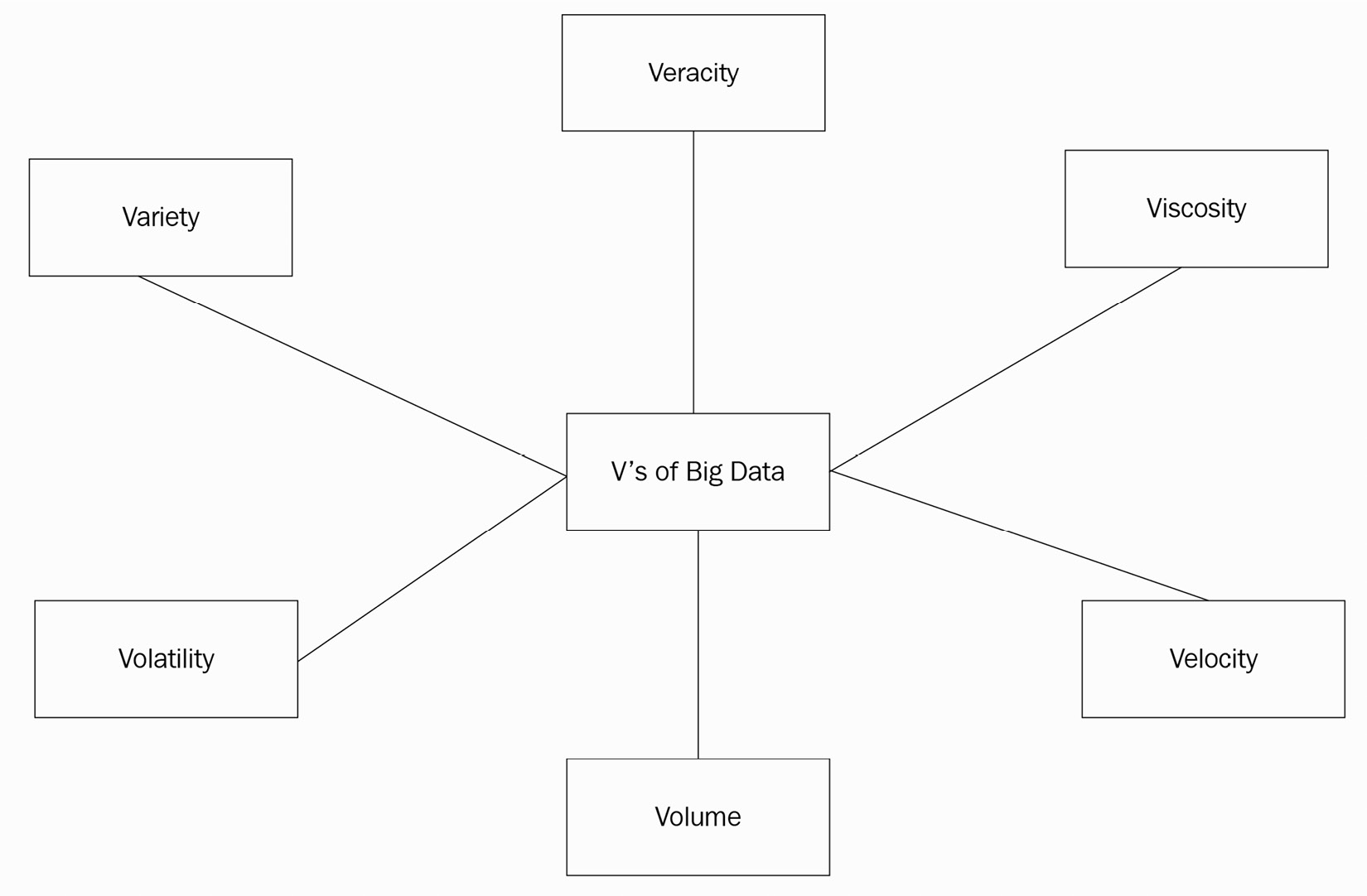
Figure 6.1 – The evolution of big data

So, you have already learned about data modeling concepts in Chapter 5, Ingesting and Streaming Data from the Edge, which is a standard way of organizing data into meaningful structures based on data types and relationships and extracting value out of it. However, collecting data, storing it in a stream or a persistent layer, and processing it quickly to take intelligent actions is only one side of the story. The next challenge is to work out how to keep a high quality of data throughout its life cycle so that it continues to generate business value for downstream applications over inconsistency or risk. For IoT workloads, this aspect is critical as the devices or gateways reside in a physical world, with intermittent connectivity, at times, being susceptible to different forms of interference. This is where the domain-driven design (DDD) approach can help.

What is domain-driven design?

To manage the quality of the data better, we need to learn how to organize data by content such as data domains or subject areas. One of the most common approaches in which to do that is through DDD, which was introduced by Eric Evans in 2003. In his book, Eric states The heart of software is its ability to solve domain-related problems for its user. All other features, vital though they may be, support this basic purpose. Therefore, DDD is an approach to software development centering around the requirements, rules, and processes of a business domain.

The DDD approach includes two core concepts: bounded context and ubiquitous language. Let's dive deeper into each of them:

• Bounded context: Bounded contexts help you to define the logical boundaries of a solution. They can be implemented on the application or business layer, as per the requirements of the organization. However, the core concept is that a bounded context should have its own application, data, and process. This allows the respective teams to clearly define the components they own in a specific domain. These boundaries are important in managing data quality and minimizing data silos, as they grow with different Vs and get redistributed with different consumers within or outside an organization. For example, with a connected HBS solution, there can be different business capabilities required by the internal business functions of HBS and their end consumers. This could include the following:
  • Internal capabilities (for the organizational entities):
    • Product engineering: The utilization of different services or features
    • Fleet operation: Monitoring fleet health
    • Information security: Monitoring the adherence to different regulatory requirements, such as GDPR
    • More such as CRM, ERP, and marketing
  • External capabilities (for the end consumer):
    • Fleet telemetry: The processing of data feeds such as a thermostat or HVAC readings from devices in near real time
    • Fleet monitoring: Capturing fleet health information or critical events such as the malfunctioning of sensors
    • Fleet analytics: Enriching telemetry data with other metadata to perform analysis factoring in different environmental factors such as time, location, and altitude

  The following diagram is an illustration of a bounded context:

Figure 6.2 – A bounded context

All of these different business capabilities can be defined as a bounded context. So, now the business capabilities have been determined, we can define the technology requirements within this bounded context to deliver the required business outcome. The general rule of thumb is that the applications, data, or processes should be cohesive and not span for consumption by other contexts. In this chapter, we are going to primarily focus on building bounded contexts for external capabilities that are required by end consumers using different technologies.

Note

However, in the real world, there can be many additional factors to bear in mind when it comes to defining a bounded context, such as an organizational structure, product ownership, and more. We will not be diving deep into these factors as they are not relevant to the topic being discussed here.

• Ubiquitous language: The second concept in DDD is ubiquitous language. Each bounded context is supposed to have its own ubiquitous language. Applications that belong together within a bounded context should all follow the same language. If the bounded context changes, the ubiquitous language is also expected to be different. This allows the bounded context to be developed and managed by one team and, therefore, aligns with the DevOps methodology as well. This operating model makes it easier for a single team, familiar with the ubiquitous language, to own and resolve different applications or data dependencies quicker.Later in this chapter, you will discover how the different bounded contexts (or workflows) are implemented using a diverse set of languages.

  Note

  The DDD model doesn't mandate how to determine the bounded context within application or data management. Therefore, it's recommended that you work backward from your use case and determine the appropriate cohesion.

So, with this foundation, let's define some design principles of data management on the cloud – some of these will be used for the remainder of the chapter.

What are the principles to design data workflows using DDD?

We will outline a set of guardrails (that is principles) to understand how to design data workloads using DDD:

• Principle 1: Manage data ownership through domains – The quality of the data along with the ease of usability are the advantages of using domains. The team that knows the data best, owns and manages it. Therefore, the data ownership is distributed as opposed to being centralized.
• Principle 2: Define domains using bounded contexts – A domain implements a bounded context, which, in turn, is linked to a business capability.
• Principle 3: Link a bounded context to one or many application workloads – A bounded context can include one or many applications. If there are multiple applications, all of them are expected to deliver value for the same business capability.
• Principle 4: Share the ubiquitous language within the bounded context – Applications that are responsible for distributing data within their bounded context use the same ubiquitous language to ensure that different terminologies and data semantics do not conflict. Each bounded context has a one-to-one relationship with a conceptual data model.
• Principle 5: Preserve the original sourced data – Ingested raw data needs to be preserved as a source of truth in a centralized solution. This is often referred to as the golden dataset. This will allow different bounded contexts to repeat the processing of data in the case of failures.
• Principle 6: Associate data with metadata – With the growth of data in terms of variety and volume, it's necessary for any dataset to be easily discoverable and classified. This eases the reusability of data by different downstream applications along with establishing a data lineage.
• Principle 7: Use the right tool for the right job – Based on the data workflow such as the speed layer or the batch layer, the persistence and compute tools will be different.
• Principle 8: Tier data storage – Choose the optimal storage layer for your data based on its access patterns. By distributing the datasets into different storage services, you can build a cost-optimized storage infrastructure.
• Principle 9: Secure and govern the data pipeline – Implement control to secure and govern all data at rest and in transit. A mechanism is required to only allow authorized entities to visualize, access, process, and modify data assets. This helps us to protect data confidentiality and data security.
• Principle 10: Design for Scale – Last but not least, the cloud is all about the economies of scale. So, take advantage of the managed services to scale elastically and handle any volume of data reliably.

In the remainder of the chapter, we will touch upon most of these design principles (if not all) as we dive deeper into the different design patterns, data flows, and hands-on labs.

Designing data patterns on the cloud

As data flows from the edge to the cloud securely over different channels (such as through speed or batch layers), it is a common practice to store the data in different staging areas or a centralized location based on the data velocity or data variety.These data sources act as a single source of truth and help to ensure the quality of the data for their respective bounded contexts. Therefore, in this section, we will discuss different data storage options, data flow patterns, and anti-patterns on the cloud. Let's begin with data storage.

Data storage

As we learned, in earlier chapters, since edge solutions are constrained in terms of computing resources, it's important to optimize the number of applications or the amount of data persisted locally based on the use case. On the other hand, the cloud doesn't have that constraint, as it comes with virtually unlimited resources with different compute and storage options. This makes it a perfect fit for big data applications to grow and contract based on the demand. In addition to this, it provides easy access to a global infrastructure to orchestrate data required by different downstream or end consumers in the region that is closer to them. Finally, data is more valuable when it's augmented with other data or metadata; thus, in recent times, patterns such as data lakes have become very popular. So, what is a data lake?

A data lake is a centralized, secure, and durable storage platform that allows you to ingest, store structured and unstructured data, and transform the raw data as required. You can think of data lake as a superset of the data pond concepts introduced in Chapter 5, Ingesting and Streaming Data from the Edge. Since the IoT devices or gateways are relatively low in storage, only highly valuable data that's relevant for the edge operations can be persisted locally in a data pond:

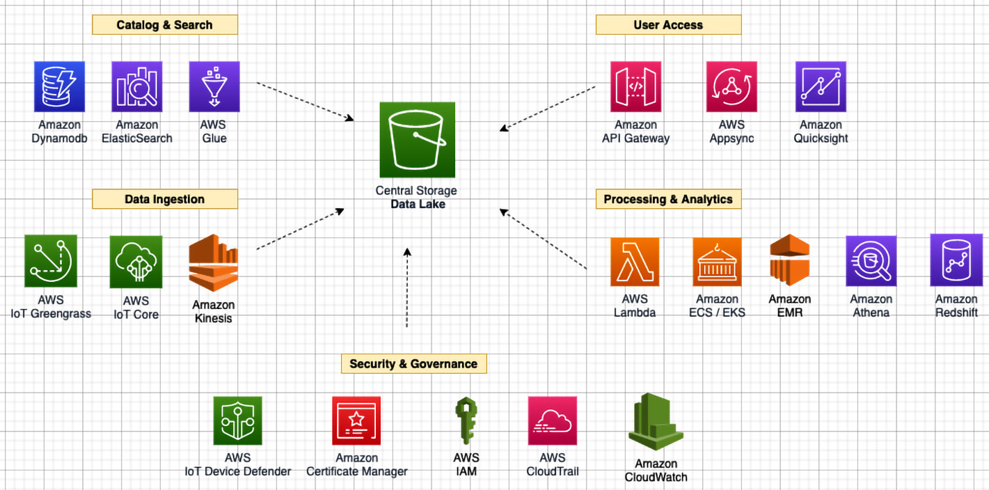
Figure 6.3 – The data lake architecture

Some of the foundational characteristics of the data lake architecture are explained here:

• There is central storage for storing raw data with minimal or no transformation securely. This is a single source of truth of data. The choice of compute, storage layer, schema, ingestion frequency, and data quality is left to the data producer. Amazon S3 is commonly chosen as the central storage since it's a highly scalable, highly durable, and cost-effective service that allows the decoupling of the compute and storage layers. AWS offers different tiering options within Amazon S3 along with a full-fledged archival service referred to as Amazon Glacier.
• There is a persistence layer for storing domain-specific data marts or transformed data in a columnar format (such as Parquet, ORC, or Avro) to achieve isolation by bounded contexts, faster performance, or lower cost. AWS offers different services such as AWS Glue for data transformation and data catalogs, Amazon Athena or Amazon Redshift for data warehouses and data marts, and Amazon EMR or Spark on EMR for managing big data processing.
• There is a persistence layer for storing transactional data ingested from the edge securely. This layer is often referred to as the Operational Data Store (ODS). AWS offers different services that can be leveraged here based on the given data structures and access patterns, such as Amazon DynamoDB, Amazon RDS, and Amazon Timestream.

You must be wondering how data from a data lake is made available to a data warehouse or an ODS. That's where data integration patterns play a key role.

Data integration patterns

Data Integration and Interoperability (DII) happens through the batch, speed, and serving layers. A common methodology in the big data world that intertwines all these layers is Extract, Transform, and Load (ETL) or Extract, Load, and Transform (ELT). We have already explained these concepts, in detail, in Chapter 5, Ingesting and Streaming Data from the Edge, and discussed how they have evolved with time into different data flow patterns such as event-driven, batch, lambda, and complex event processing. Therefore, we will not be repeating the concepts here. But in the next section, we will explain how they relate to data workflows in the cloud.

Data flow patterns

Earlier in this chapter, we discussed how bounded contexts can be used to segregate different external capabilities for end consumers, such as fleet telemetry, fleet monitoring, or fleet analytics. Now, it's time to learn how these concepts can be implemented using different data flow patterns.

Batch (or aggregated processing)

Let's consider a scenario; you discover that you have been getting a higher electricity bill for the last six months, and you would like to compare the utilization of different equipment for that time period. Alternatively, you want visibility of more granular information, such as how many times did the washing machine run during the day in the last six months? And for how long? This led to how many X watts of consumption?

This is where batch processing helps. It had been the de facto standard of the industry before event-driven architecture gained popularity and is still heavily used for different use cases such as order management, billing, payroll, financial statements, and more. In this mode of processing, a large volume of data, such as thousands or hundreds of thousands of records (or more), is typically transmitted in a file format (such as TXT or CSV), cleaned, transformed, and loaded into a relational database or data warehouse. Thereafter, the data is used for data reconciliation or analytical purposes. A typical batch processing environment also includes a job scheduler that can trigger an analytical workflow based on schedules of feed availability or those that are required by the business.

To design the fleet analytics bounded context, we have designed a batch workflow, as follows:

Figure 6.4 – The batch architecture

In this pattern, the following activities are taking place:

• Events streamed from the edge are routed through a streaming service (that is, Amazon Kinesis) to a data lake (that is, Amazon S3).
• Amazon Kinesis allows the preprocessing or enrichment of the data (if required) with additional metadata prior to persisting it to a data lake.
• The data can be crawled or transformed through an ETL engine (that is, AWS Glue) and be easily queried using a serverless analytical service (that is, Amazon Athena). Amazon Athena uses a Presto engine under the hood and is compatible with ANSI SQL.
• Different services such as Amazon S3 and Amazon Athena offer integrations with Amazon QuickSight and different third-party Business Intelligence (BI) tools through JDBC and ODBC connectors.
• Amazon S3 is highly available and durable object storage that integrates with other big data services such as a fully managed Hadoop cluster (that is, Amazon EMR) or a data warehouse (that is, Amazon Redshift).

  Fun fact

  Amazon EMR and Amazon Redshift support big data processing through decoupling of the compute layer and the storage layer, which means there is no need to copy all the data to local storage from the data lake. Therefore, processing becomes more cost-efficient and operationally optimal.

The ubiquitous language used in this bounded context includes the following:

• A REST API for stream processing on Amazon Kinesis, data processing on Amazon S3 buckets, and ETL processing on AWS Glue
• SQL for data analytics on Amazon Athena and Amazon Redshift
• MapReduce or Spark for data processing on Amazon EMR
• Rest APIs, JDBC, or ODBC connectors with Amazon QuickSight or third-party BI tools

Batch processing is powerful since it doesn't have any windowing restrictions. There is a lot of flexibility in terms of how to correlate individual data points with the entire dataset, whether it's terabytes or exabytes in size for desired analytical outcomes.

Event-driven processing

Let's consider the following scenario: you have rushed out of your home, and you get a notification after boarding your commute that you left the cooking stove on. Since you have a connected stove, you can immediately turn it off remotely from an app to avoid fire hazards. Bingo!

This looks easy, but there is a certain level of intelligence required at the local hub (such as HBS hub) and a chain of events to facilitate this workflow. These might include the following:

• Detect from motion sensors, occupancy sensors, or cameras that no one is at home.
• Capture multiple measurements from stove sensors over a period of time.
• Correlate the events to identify this as a hazard scenario using local processes at the edge.
• Stream an event to a message broker and persist it in an ODS.
• Trigger a microservice(s) to notify this event to the end user.
• Remediate the issue based on user response.

So, as you can observe, a lot is happening in a matter of seconds between the edge, the cloud, and the end user to help mitigate the hazard. This is where patterns such as event-driven architectures became very popular in the last decade or so.

Prior to EDA, polling and Webhooks were the common mechanisms in which to communicate events between different components. Polling is inefficient since there is always a lag in terms of how to fetch new updates from the data source and sync them with downstream services. Webhooks are not always the first choice, as they might require custom authorization and authentication configurations. In short, both of these methods require additional work to be integrated or have scaling issues. Therefore, you have the concept of events, which can be filtered, routed, and pushed to different other services or systems with less bandwidth and lower resource utilization since the data is transmitted as a stream of small events or datasets. Similar to the edge, streaming allows the data to be processed as it arrives without incurring any delay.

Generally, event-driven architectures come in two topologies, the mediator topology and the broker topology. We have explained them here:

• The mediator topology: There is a need for a central controller or coordinator for event processing. This is generally useful when there is a chain of steps for processing events.
• The broker topology: There is no mediator, as the events are broadcast through a broker to different backend consumers.

The broker topology is very common with edge workloads since it decouples the edge from the cloud and allows the overall solution to scale better. Therefore, for the fleet telemetry bounded context, we have designed an event-driven architecture using a broker topology, as shown in the following diagram.

In the following data flow, the events streamed from a connected HBS hub (that is, the edge) are routed over MQTT to an IoT gateway (that is, AWS IoT Core), which allows the filtering of data (if required) through an in-built rules engine and persists the data to an ODS (that is, Amazon DynamoDB). Amazon DynamoDB is a highly performant nonrelational database service that can scale automatically based on the volume of data streamed from millions of edge devices. From the previous chapter, you should already be familiar with how to model data and optimize NoSQL databases for time series data. Once the data is persisted in Amazon DynamoDB, Create, Read, Update, and Delete (CRUD) operations can be performed on top of the data using serverless functions (that is, AWS Lambda). Finally, the data is made available through an API access layer (that is, the Amazon API gateway) in a synchronous or asynchronous manner:

Figure 6.5 – Streaming architecture

The ubiquitous language used in this bounded context includes the following:

• SQL for DynamoDB table access
• Python for developing a lambda function
• A REST API for API gateway and DynamoDB access

Stream processing and EDA is powerful for many IoT use cases that require near-real-time attention such as alerting, anomaly detection, and more, as it analyzes the data as soon as it arrives. However, there is a trade-off with every architecture and EDA is no exception either. With a stream, since the processed results are made available immediately, the analysis of a particular data point cannot consider future values. Even for past values, it's restricted to a shorter time interval, which is generally specified through different windowing mechanisms (such as sliding, tumbling, and more). And that's where batch processing plays a key role.

Complex event processing

Let's consider the following scenario where you plan to reduce food wastage at your home. Therefore, every time you check-in at a grocery store, you receive a notification with a list of perishable items in your refrigerator (or food shelf), as they have not even been opened or are underutilized and are nearing their expiry date.

This might sound like an easy problem to solve, but there is a certain amount of intelligence required at the local hub (such as HBS hub) and a complex event processing workflow on the cloud to facilitate this. It might include the following:

• Based on location sharing and user behavior, the ability to recognize the pattern (or a special event) that the user plans to do grocery shopping.
• Detect from camera sensors installed in the refrigerator or on the food shelves that some of the perishable items are due to expire. Alternatively, use events from smell sensors to detect a pattern of rotten food items.
• Correlate all these patterns (that is, the user, location, and food expiry date) through state machines and apply business rules to identify the list of items that requires attention.
• Trigger a microservice(s) to notify this information to the end user.

This problem might become further complicated for a restaurant business due to the volume of perishable items and the scale at which they operate. In such a scenario, having near real-time visibility to identify waste based on current practices can help the business optimize its supply chain and save a lot of costs. So, as you can imagine, the convergence of edge and IoT with big data processing capabilities such as CEP can help unblock challenging use cases.

Processing and querying events as they arrive in small chunks or in bulk is relatively easier compared to recognizing patterns by correlating events. That's where CEP is useful. It's considered as a subset of stream processing with the focus to identify special (or complex) events by correlating events from multiple sources or by listening to telemetry data for a longer period of time. One of the common patterns to implement CEP is by building state machines.

In the following flow, the events streamed from a connected HBS hub (that is, the edge) are routed over MQTT to an IoT gateway (that is, AWS IoT Core), which filters the complex events based on set criteria and pushes them to different state machines defined within the complex event processing engine (that is, AWS IoT events). AWS IoT events is a fully managed CEP service that allows you to monitor equipment or device fleets for failure or changes in operation and, thereafter, trigger actions based on defined events:

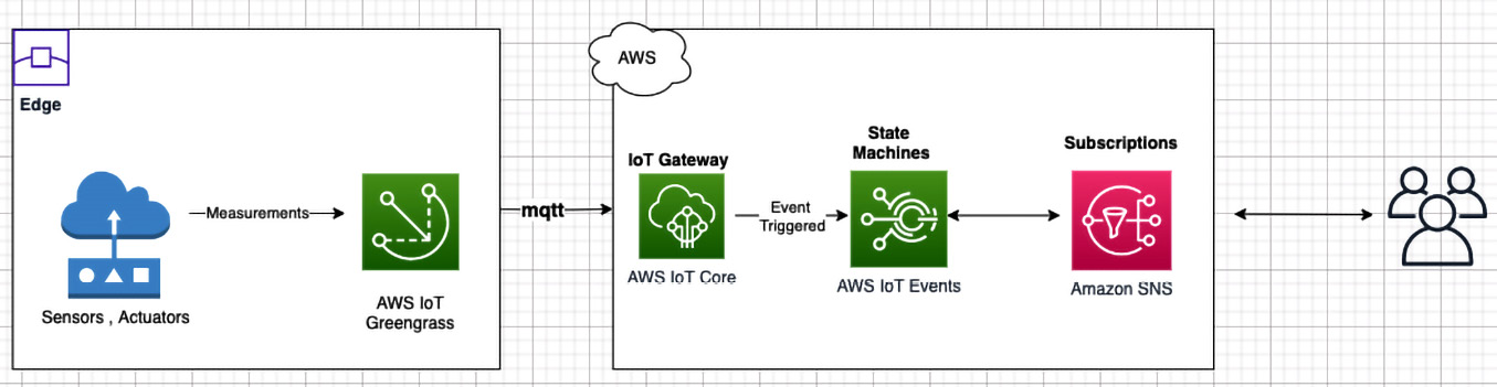
Figure 6.6 – CEP architecture

The ubiquitous language used in the fleet monitoring bounded context includes the following:

• State machines for complex event processing
• A REST API for notifications or subscriptions through Amazon Simple Notification Service (SNS)

CEP can be useful for many IoT use cases that require attention based on events from multiple sensors, timelines, or other environmental factors.

There can be many other design patterns that you need to consider in order to design a real-life IoT workload. Those could be functional or non-functional requirements such as data archival for regulatory requirements, data replication for redundancy, and disaster recovery for achieving required RTO or RPO; however, that's beyond the scope of this book, as these are general principles and not necessarily related to edge computing or IoT workloads. There are many other books or resources available on those topics if they are of interest to you.

Data flow anti-patterns for the cloud

The anti-patterns for processing data on the cloud from edge devices can be better explained using three laws – the law of physics, the law of economics, and the law of the land:

• Law of physics: For use cases where latency is critical, keeping data processing closer to the event source is usually the best approach, since we cannot beat the speed of light, and thus, the round-trip latency might not be affordable. Let's consider a scenario where an autonomous vehicle needs to apply a hard brake after detecting a pedestrian; it cannot afford the round-trip latency from the cloud. This factor is also relevant for physically remote environments, such as mining, oil, and gas facilities where there is poor or intermittent network coverage. Even for our use case here, with connected HBS, if there is a power or network outage, the hub is still required to be intelligent enough to detect intrusion by analyzing local events.
• Law of economics: The cost of compute and storage has reduced exponentially in the last few decades compared to networking cost, which might still become prohibitive at scale. Although digital transformation has led to data proliferation across different industries, much of the data is of low quality. Therefore, local aggregation and the filtering of data on the edge will allow you to publish high-value data to the cloud only reducing networking bandwidth costs.
• Law of the land: Most industries need to comply with regulations or compliance requirements related to data sovereignty. Therefore, the local retention of data in a specific facility, region, or country might turn out to be a key factor in the processing of data. Even for our use case here with connected HBS, the workload might need to be in compliance with GDPR requirements.

AWS offers different edge services for supporting use cases that need to comply with the preceding laws and are not limited to IoT services only. For example, consider the following:

• Infrastructure: AWS Local Zones, AWS Outposts, and AWS Wavelength
• Networking: Amazon CloudFront, and POP locations
• Storage: AWS Storage Gateway
• Rugged and disconnected edge devices: AWS Snowball Edge and AWS Snowcone
• Robotics: AWS Robomaker
• Video analytics: Amazon Kinesis Video Streams
• Machine learning: Amazon Sagemaker Neo, Amazon Sagemaker Edge Manager, Amazon Monitron, and AWS Panorama

The preceding services are beyond the scope of the book, and the information is only provided for you to be well informed of the breadth and depth of AWS edge services.

A hands-on approach with the lab

In this section, you will learn how to design a piece of architecture on the cloud leveraging the concepts that you have learned in this chapter. Specifically, you will continue to use the lambda architecture pattern introduced in Chapter 5, Ingesting and Streaming Data from the Edge, to process the data on the cloud:

Figure 6.7 – Hands-on architecture

In the previous chapter, you already completed steps 1 and 4. This chapter will help you to complete steps 2, 3, 5, 6, and 7, which includes consuming the telemetry data and building an analytics pipeline for performing BI:

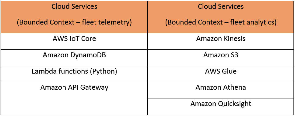
Figure 6.8 – Hands-on lab components 

In this hands-on section, your objectives include the following:

1. Query the ODS.
2. Build an API interface layer to enable data consumption.
3. Build an ETL layer for processing telemetry data in the data lake.
4. Visualize the data through a BI tool.

Building cloud resources

This lab builds on top of the cloud resources that you have already deployed in Chapter 5, Ingesting and Streaming Data from the Edge. So, please ensure you have completed the hands-on section there prior to proceeding with the following steps here. In addition, please go ahead and deploy the CloudFormation template from the chapter 6/cfn folder to create the resources required in this lab, such as the AWS API gateway, lambda functions, and AWS Glue crawler.

Note

Please retrieve the parameters required for this CloudFormation template (such as an S3 bucket) from the Output section of the deployed CloudFormation stack of Chapter 5, Ingesting and Streaming Data from the Edge.

In addition to this, you can always find the specific resource names required for this lab (such as lambda functions) from the Resources or Output sections of the deployed CloudFormation stack. It is a good practice to copy those into a notepad locally so that you can refer to them quickly.

Once the CloudFormation has been deployed successfully, please continue with the following steps.

Querying the ODS

Navigate to the AWS console and try to generate insights from the data persisted in the operational (or transactional) data store. As you learned in the previous chapter, all the near real-time data processed is persisted in a DynamoDB table (packt_sensordata):

1. To query the data, navigate to DynamoDB Console, select Tables (from the left-hand pane), click on the table, and then click on View items.
2. Click on the Query tab. Put a value of 1 into the device_id partition key and click on Run. This should return a set of data points with all the attributes.
3. Expand the filters section, and add filters to the following attributes:  
   • Attribute name – temperature.
   • Type – Number.
   • Condition – Greater than or Equal.
   • Value – 50.  
   • Click Add filter.
   • Attribute name – humidity.
   • Type – Number.
   • Condition – Greater than or Equal.
   • Value – 35.  
   • Click on Run.

   Here, the query interface allows you to filter the data quickly based on different criteria. If you are familiar with SQL, you can also try the PartiQL editor, which is on the DynamoDB console.

4. Additionally, DynamoDB allows you to scan an entire table or index, but this is generally an expensive operation, particularly for a large dataset. To scan a table, click on the Scan tab (which is adjacent to Query) and then click on Run.

For better performance and faster response times, we recommend that you use Query over Scan.

AWS Lambda

In addition to having interactive query capabilities on data, you will often need to build a presentation layer and business logic for various other personas (such as consumers, fleet operators, and more) to access data. You can define the business logic layer using Lambda:

1. Navigate to the AWS Lambda console. Click on Functions (from the left-hand pane), and choose the function created using the CloudFormation template earlier.
2. Do you remember that we created two facets (getItems and putItems) during the data modeling exercise in Chapter 5, Ingesting and Streaming Data from the Edge, to access data? The following is the logic embedded in a lambda function to implement the equivalent functional construct. Please review the code to understand how the get and put functionalities work:

     try {

       switch (event.routeKey) {

         case "GET /items/{device_id}":

           var nid = String(event.pathParameters.id);

           body = await dynamo

             .query({

               TableName: "<table-name>",

               KeyConditionExpression: "id = :nid",

               ExpressionAttributeValues: {

                 ":nid" : nid

               }

             })

             .promise();

           break;

         case "GET /items":

           body = await dynamo.scan({ TableName: "<table-name>" }).promise();

           break;

         case "PUT /items":

           let requestJSON = JSON.parse(event.body);

           await dynamo

             .put({

               TableName: "<table-name>",

               Item: {

                 device_id: requestJSON.id,

                 temperature: requestJSON.temperature,

                 humidity: requestJSON.humidity,

                 device_name: requestJSON.device_name

               }

             })

             .promise();

           body = `Put item ${requestJSON.id}`;

           break;

         default:

           throw new Error(`Unsupported route: "${event.routeKey}"`);

       }

     } catch (err) {

       statusCode = 400;

       body = err.message;

     } finally {

       body = JSON.stringify(body);

     }

     return {

       statusCode,

       body,

       headers

     };};

Please note that here, we are using lambda functions. This is because serverless functions have become a common pattern to process event-driven data in near real time. Since it alleviates the need for you to manage or operate any servers throughout the life cycle of the application, your only responsibility is to write the code in a supported language and upload it to the Lambda console.

Fun fact

AWS IoT Greengrass provides a Lambda runtime environment for the edge along with different languages such as Python, Java, Node.js, and C++. That means you don't need to manage two different code bases (such as embedded and cloud) or multiple development teams. This will cut down your development time, enable a uniform development stack from the edge to the cloud, and accelerate your time to market.

Amazon API gateway

Now the business logic has been developed using the lambda function, let's create the HTTP interface (aka the presentation layer) using Amazon API gateway. This is a managed service for creating, managing, and deploying APIs at scale:

1. Navigate to the Amazon API Gateway console, click on APIs (from the left-hand pane), and choose the API (MyPacktAPI) created using the CloudFormation template.
2. Expand the Develop section (in the left-hand pane). Click on Routes to check the created REST methods.
3. You should observe the following operations:

   /items GET – allows accessing all the items on the DynamoDB table (can be an expensive operation)

4. Continue underneath the Develop drop-down menu. Click on Authorization and check the respective operations. We have not attached any authorizer in this lab, but it's recommended for real-world workloads. API gateway offers different forms of authorizers, including built-in IAM integrations, JSON Web Tokens (JWT), or custom logic using lambda functions.
5. Next, click on Integrations (underneath Develop) and explore the different REST operations (such as /items GET). On the right-hand pane, you will see the associated lambda functions. For simplicity, we are using the same lambda function here for all operations, but you can choose other functions or targets such as Amazon SQS, Amazon Kinesis, a private resource in your VPC, or any other HTTP URI if required for your real-world use case.
6. There are many additional options offered by API gateway that relate to CORS, reimport/export, and throttling, but they are not considered in the scope of this lab. Instead, we will focus on executing the HTTP APIs and retrieving the sensor data.
7. Click on the API tab (in the left-hand pane), copy the invoke URL underneath Stages, and run the following commands to retrieve (or GET) items from your device Terminal:

   a. Query all items from the table

   curl https://xxxxxxxx.executeapi.<region>.amazonaws.com/items

   You should see a long list of items on our Terminal that has been retrieved from the dynamodb table.

Amazon API gateway allows you to create different types of APIs, and the one configured earlier falls into the HTTP API category that allows access to lambda functions and other HTTP endpoints. Additionally, we could have used the REST APIs here, but the HTTP option was chosen for its simplicity of use, as it can automatically stage and deploy the required APIs without any additional effort and can be more cost-effective. In summary, you have now completed implementing the bounded context of an ODS through querying or API interfaces.

Building the analytics workflow

In this next section, you will build an analytics pipeline on the batch data persisted on Amazon S3 (that is, the data lake). To achieve this, you can use AWS Glue to crawl data and generate a data catalog. Thereafter, you will use Athena for interactive querying and use QuickSight for visualizing data through charts/dashboards.

AWS Glue

AWS Glue is a managed service that offers many ETL functionalities, such as data crawlers, data catalogs, batch jobs, integration with CI/CD pipelines, Jupyter notebook integration, and more. Primarily, you will use the data crawler and cataloging capabilities in this lab. We feel that might be sufficient for IoT professionals since data engineers will be mostly responsible for these activities in the real world. However, if you believe in learning and are curious, please feel free to play with the other features:

1. Navigate to the AWS Glue console, click on Crawlers (from the left-hand pane), and select the crawler created earlier using the CloudFormation template.
2. Review some of the key attributes of the crawler definition, such as the following:
   • State: Is the crawler ready to run?
   • Schedule: Is the frequency of the crawler set correctly?
   • Data store: S3.
   • Include path: Is the location of the dataset correct? This should point to the raw sensor data bucket.
   • Configuration options: Is the table definition being updated in the catalog based on upstream changes?
3. Additionally, Glue allows you to process different data formats through its classifier functionality. You can process the most common data formats such as Grok, XML, JSON, and CSV with its built-in classifiers along with specifying custom patterns if you have data in a proprietary format.
4. Here, the crawler should run on the specified schedule configured through CloudFormation; however, you can also run it on demand by clicking on Run Crawler. If you do the same, please wait for the crawler to complete the transition from the starting -> running -> stopping -> ready status.
5. Now the data crawling is complete, navigate to Tables (from the left-hand pane) and confirm whether a table (or tables) resembling the name of *packt* has been created. If you have a lot of tables already created, another quick option is to use the search button and filter on Database: packt_gluedb.
6. Click on the table to verify the properties, such as the database, the location, the input/output formats, and the table schema. Confirm the schema is showing the attributes that you are interested in retaining. If not, you can click on Edit schema and make the necessary changes:
   

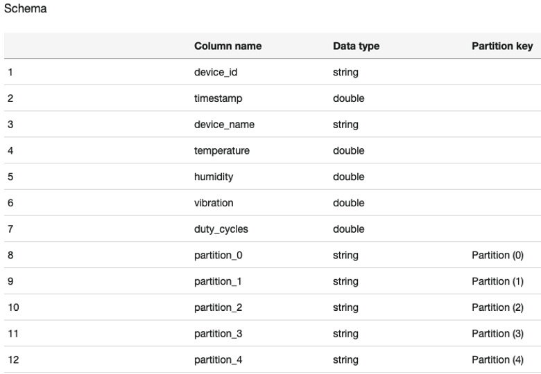
   Figure 6.9 – The table schema in Glue

7. Keep a note of the database and the table name, as you will need them in the next two sections.

In this lab, you used a crawler with a single data source only; however, you can add multiple data sources if required by your use case. Once the data catalog is updated and the data (or metadata) is available, you can consume it through different AWS services. You might need to often clean, filter, or transform your data as well. However, these responsibilities are not generally performed by the IoT practitioners and, primarily, fall with the data analysts or data scientists.

Amazon Athena

Amazon Athena acts as a serverless data warehouse where you run analytical queries on the data that's curated by an ETL engine such as Glue. Athena uses a schema-on-read approach; thus, a schema is projected onto your data when you run a query. And since Athena enables the decoupling of the compute and storage layers, you can connect to different data lake services such as S3 to run these queries on. Athena uses Apache Hive for DDL operations such as defining tables and creating databases. For the different functions supported through queries, Presto is used under the hood. Both Hive and Presto are open source SQL engines:

1. Navigate to the AWS Athena console, and choose Data Sources from the left-hand pane.
2. Keep the data source as default and choose the database name of packt_gluedb:
   • This was created in the previous section by the Glue crawler automatically after scanning the S3 destination bucket, which is storing the batched sensor data.
3. This should populate the list of tables created under this database.
4. Click on the three dots adjacent to the table resembling the name of *mysensordatabucket* and select Preview table. This should automatically build and execute the SQL query.

This should bring up the data results with only 10 records. If you would like to view the entire dataset, please remove the 10-parameter limit from the end of the query. If you are familiar with SQL, please feel free to tweak the query and play with different attributes or join conditions.

Note

Here, you processed JSON data streamed from an HBS hub device. But what if your organization wants to leverage a more lightweight data format? Athena offers native support for various data formats such as CSV, AVRO, Parquet, and ORC through the use of serializer-deserializer (SerDe) libraries. Even complex schemas are supported through regular expressions.  

So far, you have crawled the data from the data lake, created the tables, and successfully queried the data. Now, in the final step, let's learn how to build dashboards and charts that can enable BI on this data.

QuickSight

As an IoT practitioner, building business dashboards might not be part of your core responsibilities. However, some basic knowledge is always useful. If you think of traditional BI solutions, it might take data engineers weeks or months to build complex interactive ad hoc data exploration and visualization capabilities. Therefore, business users are constrained to pre-canned reports and preselected queries. Also, these traditional BI solutions require significant upfront investments and don't perform as well at scale as the size of data sources grow. That's where Amazon QuickSight helps. It's a managed service that's easy to use, highly scalable, and supports complex capabilities required for business:

1. Navigate to the Amazon QuickSight console and complete the one-time setup, as explained here:
   • Enroll for the Standard Edition (if you have not used it before).
   • Purchase SPICE capacity for the lab
   • Note that this has a 60-day trial, so be sure to cancel the subscription after the workshop to prevent getting charged.
   • Click on your login user (in the upper-right corner), and select Manage QuickSight | Security & Permissions | Add and Remove | Check Amazon Athena | Apply.
   • Click on the QuickSight logo (in the upper-left corner) to navigate to the home page.
   • Click on your login user (in the upper-right corner) and you will observe that your region preference is listed beneath your language preference.
   • Confirm or update the region so that it matches your working region.
2. Click on New Analysis, then New dataset, and choose Athena.
3. Enter the data source name as packt-data-visualization, keep the workgroup as its default setting, and click on Create Data Source.
4. Keep the Catalog as default, choose Database, and then select the table created in step 5 of the AWS Glue section.
5. Click on Select, choose to directly query your data, and then click on Visualize again.
6. Now build the dashboard:
   • Choose a timestamp for the X-axis (select MINUTE from the Value drop-down menu).
   • Choose the other readings such as device_id, temperature, and humidity for the Y-axis (select Average from the Value drop-down menu for each reading).

Feel free to play with different fields or visual types to visualize other smart home-related information. As you might have observed, while creating the dataset, QuickSight natively supports different AWS and third-party data sources such as Salesforce, ServiceNow, Adobe Analytics, Twitter, Jira, and more. Additionally, it allows instant access to the data through mobile apps (such as iOS and Android) for business users or operations to quickly infer data insights for a specific workload along with integrations to machine learning augmentation.

Congratulations! You have completed the entire life cycle of data processing and data consumption on the cloud using different AWS applications and data services. Now, let's wrap up this chapter with a summary and knowledge-check questions.

Challenge zone (Optional)

In the Amazon API gateway section, you built an interface to retrieve all the items from the dynamodb table. However, what if you need to extract a specific item (or set of items) for a particular device such as HVAC? That can be a less costly operation compared to scanning all data.

Hint: You need to define a route such as GET /items {device_id}. Check the lambda function to gain a better understanding of how it will map to the backend logic.

Summary

In this chapter, you were introduced to big data concepts relevant to IoT workloads. You learned how to design data flows using DDD approach along with different data storage and data integration patterns that are common with IoT workloads. You implemented a lambda architecture to process fleet telemetry data and an analytical pipeline. Finally, you validated the workflow by consuming data through the APIs and visualizing it through business dashboards. In the next chapter, you will learn how all of this data can be used to build, train, and deploy machine learning models.

Knowledge check

Before moving on to the next chapter, test your knowledge by answering these questions. The answers can be found at the end of the book:

1. Can you think of at least two benefits of domain-driven design from the standpoint of edge workloads?
2. True or false: bounded context and ubiquitous language are the same.
3. What do you think is necessary to have an operational datastore or a data lake/data warehouse?
4. Can you recall the design pattern name that brings together streaming and batch workflows?
5. What strategy could you incorporate to transform raw data on the cloud?
6. True or false: You cannot access data from a NoSQL data store through APIs.
7. When would you use a mediator versus broker topology for the event-driven workload?
8. Can you think of at least one benefit of using a serverless function for processing IoT data?
9. What business intelligence (BI) services can you use for data exposition to end consumers?
10. True or false: JSON is the most optimized data format for big data processing on the cloud.
11. How would you build an API interface on top of your operational data store (or data lake)?

References

Take a look at the following resources for additional information on the concepts discussed in this chapter:

• Data Management – Body of Knowledge: https://www.dama.org/cpages/body-of-knowledge 
• Domain-Driven Design by Eric Evans: https://www.amazon.com/Domain-Driven-Design-Tackling-Complexity-Software-ebook/dp/B00794TAUG
• Domain Language: https://www.domainlanguage.com/ddd
• Big Data on AWS: https://aws.amazon.com/big-data/use-cases/
• AWS Serverless Data Analytics Pipeline: https://d1.awsstatic.com/whitepapers/aws-serverless-data-analytics-pipeline.pdf
• Modern serverless architecture on AWS: https://d1.awsstatic.com/architecture-diagrams/ArchitectureDiagrams/mobile-web-serverless-RA.pdf?did=wp_card&trk=wp_card
• BI Tools: https://aws.amazon.com/blogs/big-data/tag/bi-tools/