Chapter 7: Machine Learning Workloads at the Edge

The growth of edge computing is not only driven by advancements in computationally efficient hardware devices but also by the advent of different software technologies that were only available on the cloud (or on-premises infrastructure) a decade back. For example, think of smartphones, smartwatches, or personal assistants such as Amazon Alexa that bring a mix of powerful hardware and software capabilities to consumers. Capabilities such as unlocking your phone or garage doors using facial recognition, having a conversation with Alexa using natural language, or riding an autonomous car have become the new normal. Thus, a need for cyber-physical systems to build intelligence throughout their lifetime based on continuous learning from their surroundings has become key for various workloads in today's world.

It's important to realize that most of the top technology companies (such as Apple, Amazon, Google, and Meta, formerly Facebook) use machine learning (ML) and have made it more accessible to consumers through their products. It's not a new technology, either, and has been used by industry sectors such as financial, healthcare, and industrial settings for a long time. In this chapter, we will focus on how ML capabilities can be leveraged for any internet of things (IoT) workload.

We will continue to work on the connected hub solution and learn how to develop ML capabilities on the edge (aka a Greengrass device). In the previous chapters, you have already learned about processing different types of data on the edge, and now, it's time to learn how different ML models can perform inference on this data to derive intelligent insights on the edge.

In this chapter, we will cover the following topics:

• Defining ML for IoT workloads
• Designing an ML workflow in the cloud
• Hands-on with ML workflow architecture

Technical requirements

The technical requirements for this chapter are the same as those outlined in Chapter 2, Foundations of Edge Workloads. See the full requirements in that chapter.

Defining ML for IoT workloads

ML technologies are no longer technologies of the future— they have transformed the lives of millions of people in the last few decades. So, what is ML?

"Machine Learning is the field of study that gives computers the ability to learn without being explicitly programmed."

– Arthur Samuel, 1959

Let's look at some real-world examples of ML applications for IoT workloads from the consumer and industrial segments.

First, here are some examples from the consumer segment:

• Smartphones or smartwatches that can identify your daily habits and provide recommendations related to fitness or productivity
• Personal assistants (such as Alexa, Google, and Siri) that you can interact with in a natural way for different needs such as controlling your lights and heating, ventilation, and air conditioning (HVAC)
• Smart cameras that can monitor your surroundings and detect unexpected behaviors or threats
• Smart garages that can recognize your car through its visual attributes, license plates, or even drivers' faces
• Self-driving cars that can continuously become smarter in identifying driving patterns, objects, and pedestrians in traffic

Here are some examples from the industrial segment:

• Smart factories that enable better optimization of overall equipment effectiveness (OEE)
• Better worker safety and productivity in different industrial plants, warehouses, or working sites
• Real-time quality control (QC) using computer vision (CV) or audio to identify defects
• Improving supply chain to reduce waste and enhance customer experience such as 1 hour or 15 mins delivery (with drones) from Amazon.com

To build the aforementioned capabilities, customers have used different ML frameworks and algorithms. For the sake of brevity, we are not going to cover every ML framework that exists today. We believe it's an area of data science that doesn't fit into the daily responsibilities of an IoT practitioner. But if you are interested in diving deeper, there are many books on ML/artificial intelligence (AI) available. Thus, our focus in this chapter will be to learn a bit about the history and core concepts of ML systems, and the approach to integrating ML with IoT and edge workloads.

What is the history of ML?

Today, as humans, we can communicate with machines of different kinds (from mobiles to self-driving cars) using voice, vision, or touch. This would not have been possible without the adoption of ML technologies. This is just the beginning, and ML will be more accessible in the years to come to transform our lives in different ways. You can take a quick tour through the history of this amazing technology in this article published by Forbes: https://www.forbes.com/sites/bernardmarr/2016/02/19/a-short-history-of-machine-learning-every-manager-should-read/?sh=1ca6cea115e7.

Beyond the research community, technology companies such as Amazon.com, Google, and others also started adopting ML technologies in the late 1990s. For example, Amazon.com used ML algorithms to learn about the reading preferences of their customers and built a model to notify them of new book releases matching their interests or genres. Google used ML for their search engine, Microsoft used it for identifying spam in emails, and so on. Since then, this technology has been adopted by many other industries for a plethora of use cases.

Now that we have learned a bit about the background of ML, let's now try to understand the foundation of ML.

What are the different types of ML systems?

Similar to distributed data systems, where there are different kinds of technologies to process different types of data, ML systems also come in different flavors. If we classify them into broader categories, the distinction can be described in this way:

• Supervised ML (SML)—In this method of ML, the model is trained with a labeled dataset and requires human supervision (or a teacher). For example, let's consider a scenario where we need a connected hub solution to identify different objects such as cats, dogs, humans (or seasonal birds?) who might have intruded onto your premises. Thus, the images are required to be labeled by a human (or humans), and the models will be trained on that data using a classification algorithm before they are ready (that is, the models) to predict the outcomes. In the following screenshot, you can see some objects are already labeled while the rest are not. So, humans are required to do their due diligence with labeling for the model to be effective:

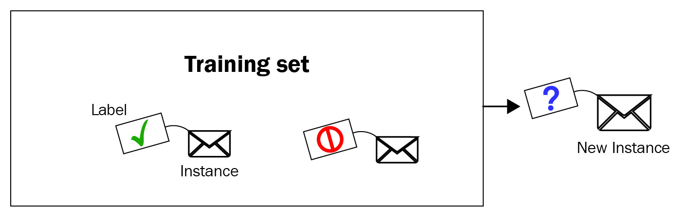
Figure 7.1 – A labeled training set of image classification

The length of the training and the volume and quality of the data will determine the accuracy of the model.

• Unsupervised ML (UML)—In this method of ML, the model is trained with an unlabeled dataset and requires no human supervision (or self-teaching). For example, let's consider that you have a new intruder on your premises, such as a deer, a wolf (or a tiger?), and you expect the model to detect that as an anomaly and notify you. In the following screenshot, you can see that none of the images is labeled and the model is required to figure out the anomaly on its own:

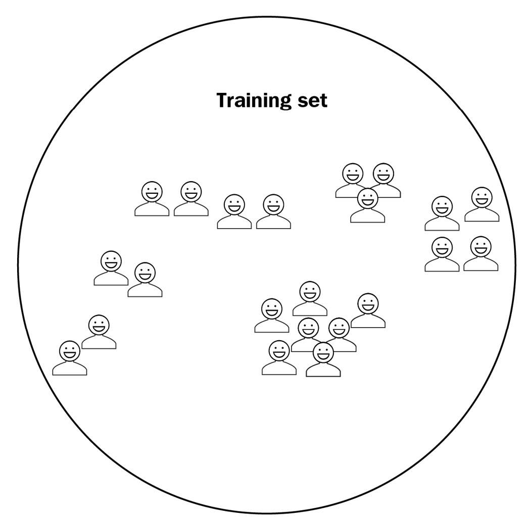
Figure 7.2 – An unlabeled training set of image classification

Considering the training dataset did not have pictures of a deer, a wolf, or a tiger, the model needs to be smart enough to identify that as an anomaly (or a novelty detection) using algorithms such as random forest.

• Semi-supervised ML (SSML)—In this method of ML, the model is trained with a dataset that is a mix of unlabeled and labeled data (think of on-demand teaching where you need to learn most of the content on your own). So, let's consider a scenario where you collected pictures of your guests from a party thrown at your home. Different guests show up in different photos and most of them are not labeled, which is the unsupervised part of the algorithm (such as clustering). Now, as the host of the party, if you label the unique individuals once in the dataset, the ML model can immediately recognize those individuals in other pictures on its own, as shown in the following diagram:

Figure 7.3 – SSML

This might be very useful if you want to search photos of individuals or families and share these with them (who cares about photos of other families, huh?).

• Reinforcement learning (RL)—In this method of ML, the model is trained to make a sequence of decisions in an environment and maximize a long-term objective. The model learns through an iterative process of trial and error. An agent such as a physical or virtual device uses this model to take actions guided by a policy at a given environment state and reaches a new state. This makes the agent eligible for a reward (positive or negative), and the agent continues to iterate on this process until it leads to the most optimal long-term rewards. The entire life cycle of an agent progressing from an initial state to a final state is called an episode.

  For example, using RL, you can train a robot to take pictures of all guests from a party thrown at your home. The robot will stay on a specific track and capture images from that environment. It will receive a positive reward if it stays on track and captures acceptable images and a negative reward for going off track or capturing distorted snaps. As it continues to iterate through this process, eventually it will learn how to maximize its long-term objectives of capturing glorious images. The following diagram reflects this process of RL:

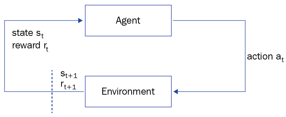
Figure 7.4 – RL

We have explained a broader category of ML in the preceding diagram; however, there is a plethora of frameworks and algorithms that are beyond the scope of this book. So, in the next section, we will focus on the most common ones that can apply to data generated from IoT and edge workloads.

Taxonomy of ML with IoT workloads

The three most common uses of ML in IoT are in the fields of classification, regression, and clustering, as depicted in the following diagram:

Figure 7.5 – Summarized taxonomy of ML algorithms

Let's discuss the nomenclature in the preceding diagram in more detail, as follows:

• Classification—Classification is an SML technique where you start with a set of observed values and derive some conclusion about unknown data. In the real world, classification can be used in image classification, speech recognition, drugs classification, sentiment analysis, biometric identification, and more.
• Regression—Regression is an SML technique where you can predict a continuous value. The prediction happens by estimating the relationship between the dependent variable (Y) and one or more independent variables (X) using a best-fit straight line. In the real world, regression can be applied to forecasting the temperature tomorrow, the price of energy utilization, the price of gold, and so on.
• Clustering—Clustering is a UML algorithm where you can group unlabeled data points. This is used very often for statistical analysis. The grouping of unlabeled data points in a dataset is performed by identifying data points in a dataset that share common properties and features. In the real world, this algorithm can be applied to market segmentation, medical imaging, anomaly detection, and social network analysis.

In the hands-on lab section of this chapter, you will learn how to use a classification algorithm to classify objects (such as cars and pets).

Why is ML accessible at the edge today?

We have already introduced you to three laws of edge computing in Chapter 6, Processing and Consuming Data on the Cloud: Law of Physics (latency-sensitive use cases), Law of Economics (cost-sensitive use cases), and Law of the Land (data-sensitive use cases). Based on these laws, we can identify various use cases in today's world, especially related to IoT and the edge, where it makes a lot of sense to process and generate insights from the data locally on the device or the gateway itself rather than publishing them continuously to the cloud.

However, the constraint is the limited resources (such as central processing unit (CPU), graphics processing unit (GPU), memory, network, and energy) available on these edge devices or gateways. Thus, it is recommended to take advantage of the computing power of the cloud to build and train ML models using the preferred framework (such as MXNET, TensorFlow, PyTorch, Caffe, or Gluon) and then deploy the model to the edge for inferencing.

For example, if there is a lot of noisy data generated in a smart home from a baby crying, a dog barking, or construction noises from the surroundings, the ML model can identify that as noisy data, trigger any specified action locally—such as an alert to check on the baby or the pet—but avoid publishing those data points to the cloud. In that way, a large amount of intermittent data that's of less long-term value can be filtered out at the site itself.

ML at the edge is an evolving space and there are many emerging frameworks and hardware offerings available today from different vendors, a few of which are listed in the following tables.

Here are common ML frameworks for the edge:

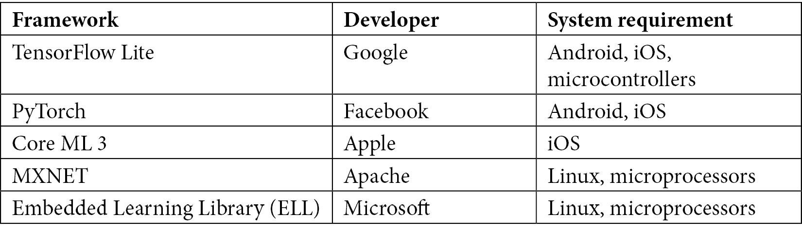
Figure 7.6 – Common ML frameworks for the edge

Here are common hardware stacks for performing ML at the edge:

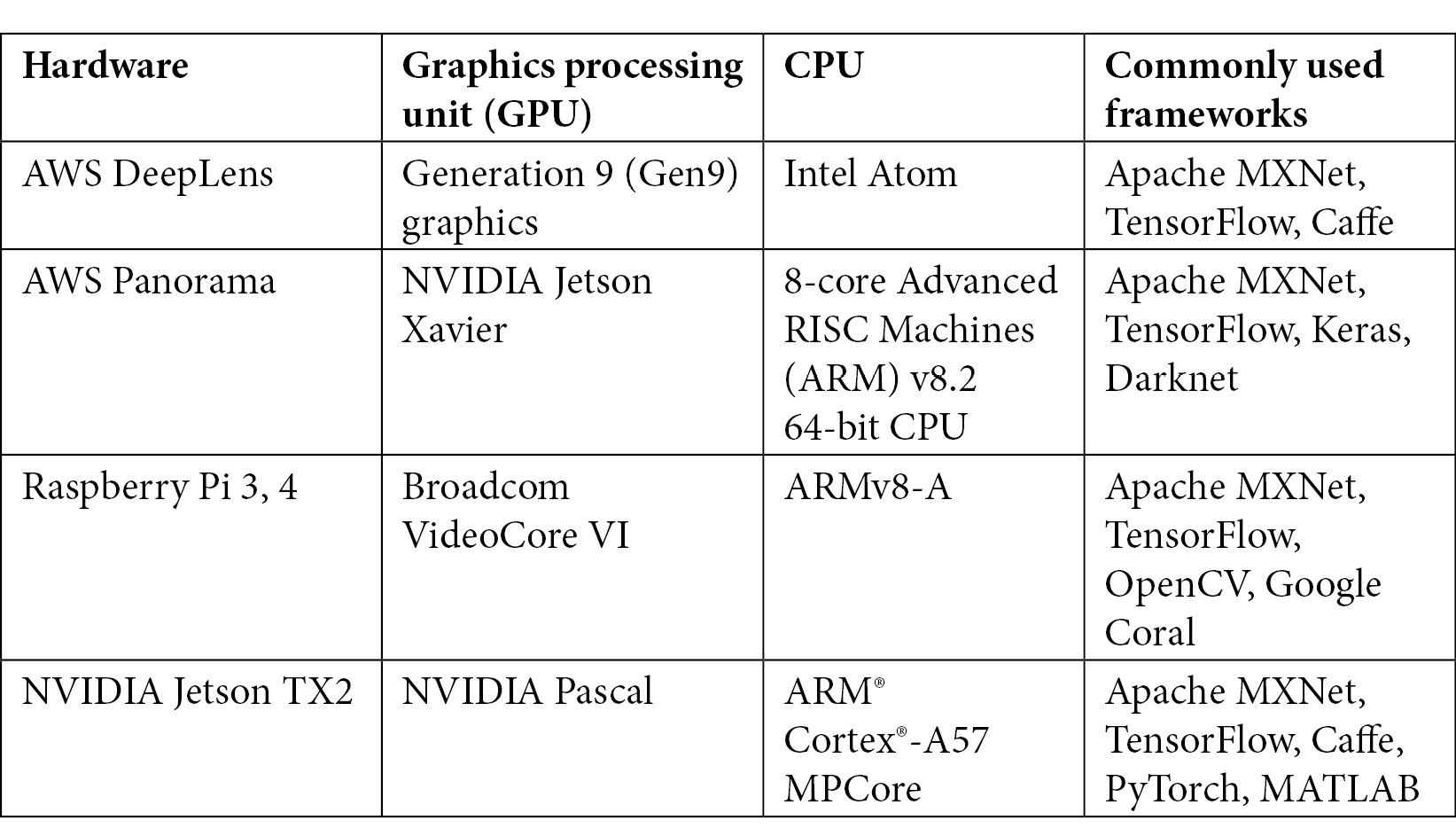
Figure 7.7 – Common hardware stacks for performing ML at the edge

You are already using Raspberry Pi as the underlying hardware for the different labs in this book. In the Hands-on with ML architecture section, you will learn how to train Apache MXNET-based ML models in the cloud and deploy them at the edge for inferencing. With this background, let's discuss how to get started with building ML applications for the edge.

Designing an ML workflow in the cloud

ML is an end-to-end (E2E) iterative process consisting of multiple phases. As we explain the different phases throughout the rest of the book, we will align to the general guidelines provided by Cross Industry Standard Process for Data Mining (CRISP-DM) consortium. The CRISP-DM reference model was conceived in late 1996 by three pioneers of the emerging data mining market and continued to evolve through participation from multiple organizations and service suppliers across various industry segments. The following diagram shows the different phases of the CRISP-DM reference model:

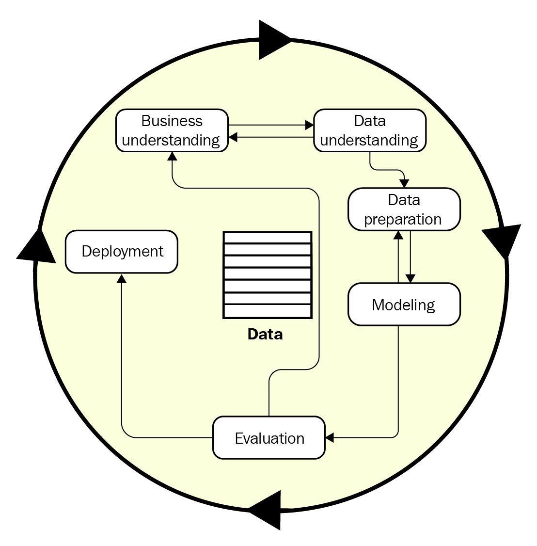
Figure 7.8 – Phases of the CRISP-DM reference model (redrawn from https://www.the-modeling-agency.com/crisp-dm.pdf)

This model is still considered a baseline and a proven tool for conducting successful data mining projects as its application is neutral and applies well to a wide variety of ML pipelines and workloads. Using the preceding reference model (Figure 7.5) as the foundation, the life cycle of an ML project can be expanded to the following activities:

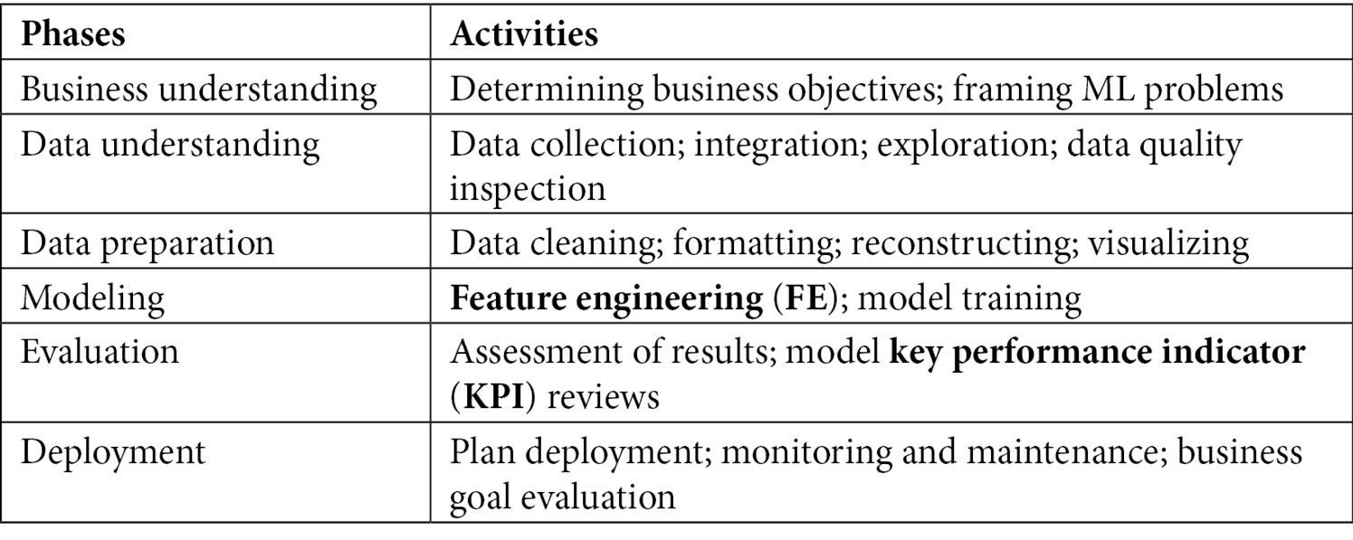
Figure 7.9 – Life cycle of an ML project

The workflow of the preceding ML activities can be visually depicted as follows:

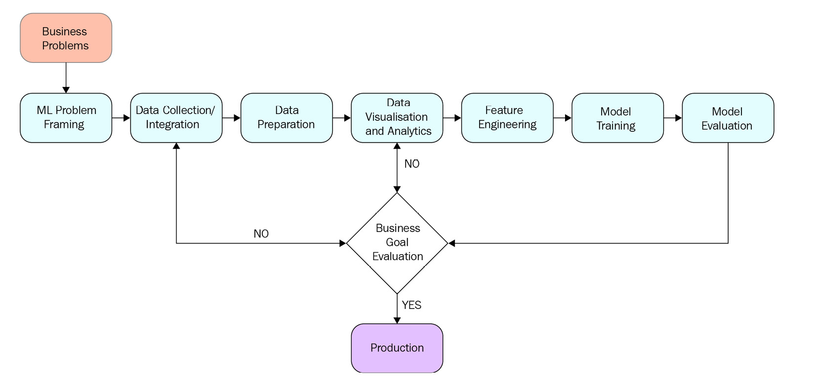
Figure 7.10 – E2E ML process

In the following section, we will elaborate on these concepts in detail by using an image classification scenario for your connected home.

Business understanding and problem framing

The first phase is working backward from the use case and understanding the requirements from a business perspective. Once that's clear, the business context gets translated to the technical requirements (such as the need for ML technologies) to achieve the required business outcomes. Does this concept sound familiar? If yes, congrats—you were able to relate to the concepts of domain-driven design (DDD), introduced in Chapter 6, Processing and Consuming Data on the Cloud. The ML capabilities can be treated as just another bounded context with its own set of ubiquitous languages.

But problem-solving using ML can be different, and here is a great quote from Peter Norvig (Director of Research at Google) on that:

"Machine Learning changes the way you think about a problem. The focus shifts from a mathematical science to a natural science, running experiments and using statistics, not logic, to analyze its results."

An organization needs to clearly identify whether the business problem they are trying to solve is an ML problem. If the problem can be solved using traditional programming methods, building ML models might be overkill. For example, if you plan to forecast the future revenue of your business for a specific quarter based on historical data, traditional analytical methods might be sufficient. But if you start factoring prediction of other variables such as weather, competitor campaigns, promotions, economy, this becomes a better fit for an ML problem. So, as a rule of thumb, always try to start your ML journey with the following questions:

• What problem is my organization or product facing?

  Let's consider a scenario where you are trying to solve the problem of securing your family, pets, and neighbors from incoming traffic around your parking space.

• Would it be a good problem to solve using ML or classic analytics methods?

  Here, a connected Home Base Solutions (HBS) hub is required to identify any living things in the parking space when a vehicle approaches or departs the area. This problem cannot be solved using a classic analytics method because you won't have the schedule available for every visitor, neighbor, or delivery van for your area. Thus, the hub can detect the movement of a vehicle(s) using motion sensors, capture different images from the surroundings (using the installed camera), and run real-time inferences to detect any objects around it. If that's found, it will alert the driver, kids, or pets in real time and avoid accidents.

  Earlier, computer vision (CV) models relied on raw pixel data as an input, but this was found to be inefficient due to several other factors such as different backgrounds behind the object, lighting, camera angle, or focus. Thus, image classification is clearly an ML problem.

• If it's an ML problem, do I have enough data of optimal quality?

  Considering the objects in scope here are generic—such as humans, cats, or cars—we can rely on public datasets such as Caltech-256. This dataset contains more than 30,000 images of 256 different types of objects.  

  This is often the most common question we come across: How much data is enough for training? It really depends.

  You should have at least a few thousand data points for basic linear models, and hundreds of thousands for neural networks (such as with image classification, as previously mentioned). More data of optimal quality enables the model to predict smarter. If you have less data or data of poor quality, the recommendation is to consider a purpose-built AI service non-ML solution first. I often like to quote that with data, it's always garbage in = garbage out. Thus, if you have questionable data quality, it is of less value to a classic analytics method or an ML process. Additionally, an ML process is more expensive as you will waste a lot of time and resources and incur costs to train models with questionable performance.

Now, let's assume that you have met the preceding requirements and identified that the problem you are trying to solve is truly an ML one. In that case, you can choose the following best practices to summarize the problem framing:

1. Formulate the ML problem into a set of questions with its respective inputs and desired outputs.
2. Define tangible performance metrics for the project, such as accuracy, prediction, or latency.
3. Establish the definition of success for the project.
4. Frame a strategy for data sourcing and data annotation.
5. Start simple—build a model that is easy to interpret, test, debug, and manage.

Data collection or integration

In this of the E2E ML process, you will identify a dataset that will feed as an input to the ML pipeline and evaluate the appropriate means to collect that. In the previous chapters, you have learned that for different IoT use cases, AWS provides a number of ways to ingest the raw data in bulk or in real time. In other real-world scenarios, if you have petabytes (PB) of historical data in your cloud platform or data centers from IoT devices and information technology (IT) systems, there are multiple ways to transfer that to a data lake in the cloud, as follows:

• Transfer over the public internet
• Transfer over a private network using a dedicated fiber channel setup from your data centers to AWS using AWS Direct Connect
• Transfer using hardware devices such as AWS Snowball, AWS Snowmobile, or AWS Snowcone, as it will take less time than transfering over the public internet

  Fun Fact

  Transporting data through snow devices is very similar to how you return a package to Amazon.com! You get hardware with an E-link screen acting as the return label, where the data can be loaded and shipped back to AWS data centers. If you have exabytes (EB) of data, AWS can even send you a truck for data transportation referred to as an AWS snowmobile. Please refer to the AWS documentation, How to get started with AWS Snow Family (https://docs.aws.amazon.com/snowball/index.html), to understand the required steps.

Again, consider the scenario of developing an ML model to identify vehicles approaching a parking-space area. Here, you can use a training dataset from a public data repository such as Caltech, as you mostly require generic images of kids, pets, and moving objects such as cars and trucks to be classified. There will be two datasets in scope, as follows:

• Training dataset—Public dataset from Caltech to be hosted on a data lake (Amazon Simple Storage Service (Amazon S3))
• Inferencing dataset—Generated in real time on the hub

The following code enables the downloading of two datasets from a public data repository:

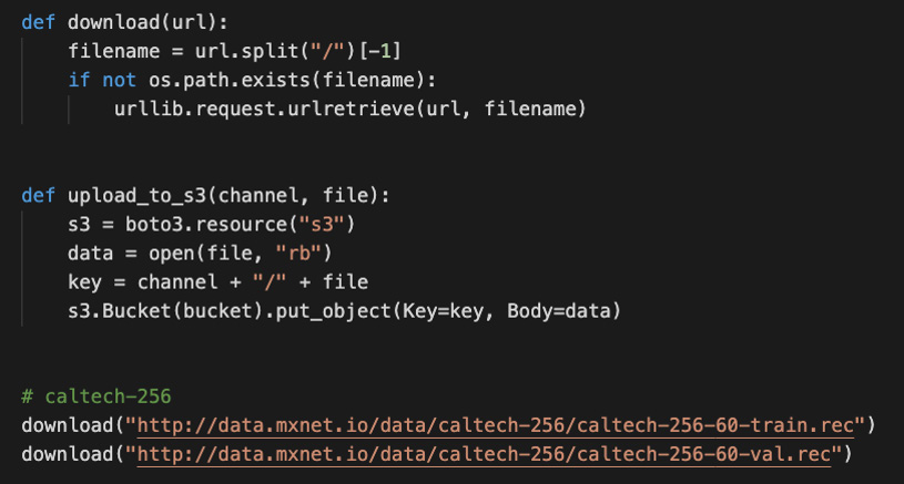
Figure 7.11 – Data understanding

For a different use case where a public dataset is not an option, your organization needs to have enough data points with optimal quality.

A summary of best practices for this phase is provided here:

• Define the various sources of data that you will use as an input to the ML pipeline
• Determine the form of data to be used as an input (that is, raw versus transformed) to the pipeline
• Use data lineage mechanisms to ensure that the data location and source are cataloged if required for further processing
• Use different AWS-managed services to collect, store, and process the data without additional heavy lifting

Data preparation

Data preparation is a key step in the pipeline as the ML models cannot perform optimally if the underlying data is not cleaned, curated, and validated. With IoT workloads, since the edge devices are co-existing in a physical environment with humans (over being hosted in a physical data center), the amount of noisy data generated can be substantial. In addition, as the dataset continues to grow from the connected ecosystem, data validation through schema comparisons can help detect if the data structure in newly obtained datasets has changed (for example, when a feature is deprecated). You can also detect if your data has started to drift—that is, the underlying statistics of the incoming data are different from the initial dataset used to train the model. Drift can happen due to an underlying trend or seasonality of the data or other factors.

Thus, the general recommendation is to start the data preparation with a small, statistically valid sample that can be iteratively improved with different strategies, such as the following:

• Checking for data anomalies
• Checking for changes in the data schema
• Checking for statistics of the different dataset versions
• Checking for data integrity, and so on

AWS provides a number of ways to help you prepare data at scale. You have already played with AWS Glue in Chapter 5, Ingesting and Streaming Data from the Edge. If you remember, AWS Glue allows you to manage the life cycle of data—such as to discover, clean, transform, and catalog. Once the data treatment is complete and the data quality meets the required standard, it can be fed as an input to an ML process.

In this chapter, we have introduced you to a different problem statement though, which is dealing with an unstructured dataset (aka images). Considering you are using a public dataset that's already labeled, you will only split the dataset into a training and a validation subset. The most common approach used by data scientists is to split the available data into a training and a test dataset, which is generally 70-30 (%) or 80-20 (%).

The following code enables the splitting of two datasets from a public data repository:

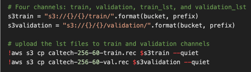
Figure 7.12 – Data preparation

In the real world, though, you may not have clean or labeled data. Thus, you can leverage services such as Amazon SageMaker Ground Truth, which has an inbuilt capability to label data (such as images, text, audio, video) automatically along with easy access to public and private human labelers. This is useful if you lack in-house ML skills or are cost-sensitive to hiring data science professionals. Ground Truth uses an ML model to automatically label the raw data and produce high-quality training datasets at a fraction of a cost. But if the model fails to label the data confidently, it will route the problem to humans for resolution. Another aspect of data preparation is to understand the patterns in your dataset.

A summary of best practices for this phase is provided here:

• Profile your data through discovery and transformation.
• Choose the right tool for the right job (such as data labeling versus tuning).
• Understand the patterns from data compositions.

Data visualization and analytics

In this phase, you can continue the data exploration through various analytics and visualization tools to assess the data fitment for ML training post profiling. You can continue to leverage services such as Amazon Athena, Amazon Quicksight, and others introduced to you in Chapter 6, Processing and Consuming Data on the Cloud.

Feature engineering (FE)

In this phase, your responsibilities as IoT professionals are very limited. This is where the data scientists will determine the unique attributes in the dataset that can be useful in training the ML model. You can think of rows as observations and columns as properties (or attributes). As data scientists, your goal is to identify the columns that matter in solving a specific business problem (aka features). For example, with image classification, the color or brand of a car is not a key feature to determine it as a vehicle. This process of selecting and transforming variables to ensure the creation of an optimized ML model is referred to as FE. Thus, the key objective of FE is to curate data in a form that an ML algorithm can use to extract patterns and infer better results.

Let's break down the different phases of FE, as follows:

• Feature creation to identify the attributes from a dataset relevant to the problem in scope, such as height and width of the pixels for images
• Feature transformation for data compatibility or quality transformation, such as resizing inputs to a fixed size or converting non-numeric to numeric data
• Feature extraction to determine a reduced set of features that offers the most value
• Feature selection to filter redundant features from a dataset by observing variance of correlation thresholds

If the number of features in a dataset becomes substantially large compared to the observations it can generate, the ML model may suffer from a problem called overfitting. On the other hand, if the number of features is limited, the model may infer a lot of incorrect predictions. This problem is referred to as underfitting. In other words, the model has trained well on the test data but is unable to apply the generalization to new or unseen datasets. Thus, feature extraction can help optimize a set of features for ML processing that are sufficient to generate a comprehensive version of the original set. Other than reducing the overfitting risk, feature extraction also speeds up the training through data compression and accuracy improvements. Different feature extraction techniques include Principal Component Analysis (PCA), Independent Component Analysis (ICA), Linear Discriminant Analysis (LDA), and Canonical Correlation Analysis (CCA).

AWS provides a number of ways to help you perform FE on your dataset at scale in an iterative way. For example, Amazon SageMaker as a managed service provides a hosted Jupyter notebook environment where you can use scikit-learn libraries to perform FE. If your organization is already invested in an extract, transform, load (ETL) framework such as AWS Glue, AWS Glue DataBrew, or a managed Hadoop framework such as Amazon Elastic MapReduce (Amazon EMR), the data scientists can perform FE and transformation there, prior to leveraging SageMaker to train and deploy the models.

Another option is using Amazon SageMaker Processing. This feature provides a fully managed environment for running analytics jobs for FE and model evaluation at scale, along with incorporating various security and compliance requirements.

Here is a summary of best practices for this phase:

• Evaluate the attributes from the dataset that fit the feature paradigm
• Consider features that are useful to solve the problem at hand and remove redundant ones
• Build an iteration mechanism to explore new features or feature combinations

Model training

The key activities in this phase include choosing an ML algorithm that's appropriate for your problem and then training the model with the preprocessed data (aka features) from the earlier phases. We have already introduced you to the ML algorithms that are most common for IoT workloads in the Taxonomy of ML with IoT workloads section. Let's dive a bit deeper into those algorithms, as follows:

• Classification—Classification can be applied in two ways; that is, binomial or multiclass. Binomial is useful when you have a set of observed values around two groups or categories, such as dog versus cat, or email being spam or not spam. Multiclass includes more than two groups or categories such as a set of flowers —roses, lilies, orchids, or tulips. Different classification techniques include decision trees, random forests, logistic regression, and naive Bayes.
• Regression—Classification is used to predict a discrete value, whereas regression is used to predict a continuous variable. Regression can be applied in three ways: least square method, linear, or logistic.
• Clustering—K-means is a very popular clustering algorithm generally used to assign a group to unlabeled data. This algorithm is fast and scalable as it uses a methodology to assign each group by computing the distance between the data point and each group center.

In the safety scenario around the parking space cited earlier, we are using a multiclass classification algorithm, since we expect the model to classify multiple categories of objects, such as humans (specially kids), cars, and animals (such as cats, dogs, and rabbits). AWS services such as SageMaker do the undifferentiated heavy lifting of creating and managing the underlying infrastructure required for the training. You can choose different types of instances, such as CPU- or GPU-enabled. In the following example, you only specify an instance type of ml.p2.xlarge along with other required parameters such as volume and instance_count, and SageMaker does the rest, using the estimator interface for instantiating and managing the infrastructure:

Figure 7.13 – ML training infrastructure

You will be using the MXNet framework in this chapter, but SageMaker allows most other ML frameworks, such as TensorFlow, PyTorch, and Gluon, to train your model.

Please note that model optimization is a critical aspect of ML where you need to train a model with different sets of parameters to identify the most performant one. SageMaker hyperparameter tuning jobs help to optimize the models using Bayesian optimization or random search techniques. As you can see in the following example, the model is getting trained using hyperparameters such as batch size and shape to solve your business problem:

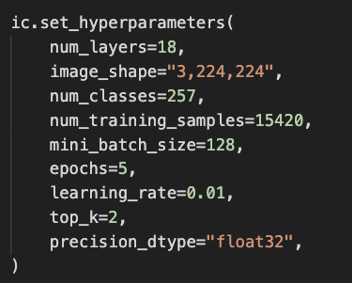
Figure 7.14 – ML training parameters

To make this process of model training easier and cost-effective for organizations new to ML, SageMaker supports automatic model tuning (through Autopilot) to automatically perform these actions on your behalf. It's also possible to use your custom ML algorithm as a container image and train it using SageMaker. For example, if you already have a homegrown image classification model that doesn't use any of the SageMaker-supported ML frameworks, you can use your model as a container image and retrain it in SageMaker without starting from scratch. SageMaker also offers a monitoring and debugging capability that allows clear visibility to the training metrics.

Here is a summary of best practices of this phase:

• Choose the right algorithm and training parameters for your data or let the managed services choose these for you
• Ensure the dataset is segregated into training and test sets
• Apply incremental learning to build the most optimized model
• Monitor the training metrics to ensure the model performance doesn't degrade over time

Model evaluation and deployment

In this phase, the model is evaluated to assess if it solves the business problem in context. If it doesn't, you can build multiple models with different business rules or methodologies (such as a different algorithm, other training parameters, and so on) until you find the optimized model that meets the business KPIs. Data scientists may often uncover inferences for other business problems in this phase as they test the model(s) against a real application. In order to evaluate the model, it can be tested against historical data (aka offline evaluation) or live data (aka online evaluation). Once the ML algorithm passes the evaluation, the next step is to deploy the model(s) to production.

The scenario for IoT/edge workloads gets a bit tricky, though, if your use cases primarily deal with offline processing and inferencing on the edge. In that case, you don't have access to the scale of the cloud, and thus the best practice is often to further optimize the models. SageMaker Neo can be useful in this scenario, as it allows you to train your model once and run anywhere in the cloud or at the edge. With this service, you can compile the model in most common frameworks (such as MXNET, TensorFlow, PyTorch, Keras) and deploy the optimized version on a target platform of your choice (such as hardware from Intel, NXP, NVIDIA, Apple, and so on). The following code helps to optimize the model based on different parameters such as OS and Architecture:

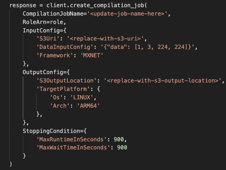
Figure 7.15 – Optimizing the model with SageMaker Neo

The way SageMaker Neo works is, its compiler uses an ML model under the hood to apply the best available performance for your model on the respective edge platform or device. Neo can optimize models to perform up to 25 times faster with no loss in accuracy and requires as little as one-tenth of the footprint compared to a non-optimized model. But how? Let's explore, as follows:

• Neo has a compiler and a runtime component.
• The Neo compiler has an application programming interface (API) that can read models developed using various frameworks. Once the read operation is complete, it converts the framework-specific functions and operations into a framework-agnostic intermediate representation.
• Once the conversion is complete, it then starts performing a set of optimizations. As a result of this optimization, binary code is generated and persisted to a shared object library, along with the model definition and parameters that are stored in separate files.
• Finally, Neo runtime APIs for the supported target platform can load and execute this compiled model to offer the required performance boost.

As you can imagine, this optimization is powerful for edge devices as they are resource-constrained. The following screenshot diagrammatically represents how you can deploy an optimized model in your production environment. In the Hands-on with ML architecture section of this chapter, you will learn how to deploy a model trained with SageMaker Neo:

Figure 7.16 – Optimizing the ML model for the hardware

Once the model is deployed, you need to monitor the performance metrics over time. This is because it's pretty common for models to function less effectively as the real-world data may start to differ from the data that was used to train the model. The SageMaker Model Monitor service can help detect deviations and alert you, the data scientists, or ML operators, to take remedial action.

Here is a summary of best practices for this phase:

• Evaluate if the model performance meets the business goals
• Identify the inferencing method required for your models (offline versus online)
• Deploy the model on the cloud with automatic scaling options or on the edge with hardware-specific optimization
• Monitor the model performance in production to identify drift and perform remediations

ML design principles

Now that you have learned about the common activities in an ML workflow, let's summarize the design principles from the steps explained in the preceding section, as follows:

• Work backward from the use case to identify if it's a problem that needs ML or that can be solved using a classic analytical approach.
• Collect enough data of optimal quality to have accurate ML models.  
• Perform profiling to understand the data relationships and compositions. Remember: garbage in = garbage out, thus data preparation is key in an ML process.
• Start with a small set of features (aka attributes) to solve a specific business problem and evolve through experimentation.
• Consider using different sets of data for training, evaluating, and inferencing purposes.
• Evaluate the accuracy of the models and continue to iterate until it's optimal for the business problem in context.
• Determine if the model needs to inference on real-time (online) or historical (offline) data.
• Host different variants of the model on the cloud or on the edge and identify the most optimal one against real-world data.
• Continuously monitor the metrics from the deployed models for accuracy, remediation, and improvement.
• Leverage managed services for offloading the heavy lifting of managing the underlying infrastructure.
• Automate the different activities of the pipeline as much as possible, such as data preparation, model training, evaluation, hosting, monitoring, and alerting.

ML anti-patterns for IoT workloads

Similar to any other distributed solutions, IoT workloads based on ML have anti-patterns as well. Here are some of them:

• Don't put all your eggs in one basket—The E2E ML process includes many activities and thus requires different personas such as the following:
  • Data engineer—For data preparation, designing ETL (or ELT) processes
  • Data scientists—For building, training, and optimizing the models
  • Development-operations (DevOps or MLOps) engineers—For building a scalable and repeatable machine learning infrastructure built with operating and monitoring mechanisms
  • IoT engineers—For building a cloud-to-edge deployment pipeline along with integration from the IoT gateway to different backend services

  In summary, expecting a single resource to perform all these activities at scale will lead to the failure of the project.

• Don't assume the requirements; get aligned—A plethora of tools is available for analytical and ML purposes and each has its pros and cons. For example, consider the following:
  • Both R and Python are popular programming languages for developing ML systems. In general, business analysts or statisticians will prefer R or other commercial solutions (such as MATLAB), while data scientists will choose Python.
  • Similarly, data scientists may have their preferred ML framework, such as TensorFlow over PyTorch. Choosing different languages or frameworks has downstream impacts—for example, the edge hardware may need to support the respective version or libraries required for inferencing the ML model.

  Thus, it's important for all the different personas engaged in ML activities to stay aligned on the business and technical requirements.

• Plan for technical debt—ML systems for IoT workloads are prone to accruing technical debt due to their data dependencies from IoT sources that are often unreliable due to their noisiness. This may also happen due to dependencies on other upstreams having inconsistent data. For example, consider the following:
  • If the composition of any feature (or a few) changes substantially, it will lead the model to behave differently in the real world. This problem is also referred to as the training-serving skew, where there is a discrepancy in how you handle data in the training and serving pipelines.
  • The reason ML workloads are different from traditional IT systems is their behavior can be determined only through real data over unit testing with a small sample.

Thus, it's key to monitor the accuracy of the model, optimize it iteratively based on the knowledge of the gathered data, and redeploy.

Hands-on with ML architecture

In this section, you will deploy a solution on a connected HBS hub that will require you to build and train ML models on the cloud and then deploy them to the edge for inferencing. The following screenshot shows the architecture of the lab with the highlighted steps (1-5) that you will complete:

Figure 7.17 – Hands-on ML architecture

Your objectives include the following, which are highlighted as distinct steps in the preceding architecture:

• Build the ML workflow using Amazon SageMaker
• Deploy the ML model from the cloud to the edge using AWS IoT Greengrass
• Perform ML inferencing on the edge and visualize the results

The following table shows the list of components you will use during the lab:

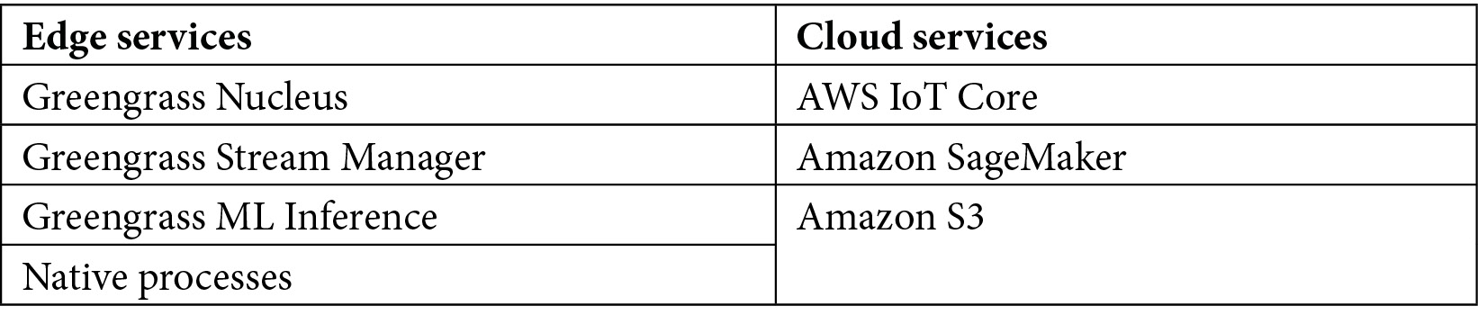
Figure 7.18 – Hands-on lab components

Building the ML workflow

In this section, you will build, train, and test the ML model using Amazon SageMaker Studio.

Note

Training models using Amazon SageMaker will incur additional cost. If you want to save on that, please use a trained ML model available in GitHub for your platform and skip to the next section, that is, Deploying the model from cloud to the edge.

Amazon Sagemaker Studio is a web-based integrated development environment (IDE) that enables data scientists (or ML engineers) with a single-stop shop for all things ML. To train the model, you will use a public dataset from Caltech that has a collection of over 30,000 images across 256 object categories. Let's begin. Proceed as follows:

1. Please navigate to the Amazon SageMaker console and select SageMaker Domain Studio (from the left pane). If this is the first time you are interacting with the studio, you will be prompted to complete a one-time setup. Please choose Quick setup, click Submit, choose Default VPC with a subnet (s) of your choice, then click Save and continue.
2. It will take a few minutes for the studio to be set up. Please wait until the status shows Ready and then click Launch app -> Studio.
3. This should open up the SageMaker Studio (aka Jupyter console) for you. In case you are new to Jupyter, consider this as an IDE for developing ML models similar to Eclipse, Visual Studio, and so on, used for developing distributed applications.
4. Please upload the Jupyter notebook (Image-Classification*.ipynb) and the synset.txt file from the chapter7/notebook folder using the Upload file button in the top-left pane.
5. Double-click to open the Jupyter notebook and choose the Python runtime and kernel, as shown in the following screenshot:
   

   Figure 7.19 – Jupyter notebook kernel

6. Choosing a kernel is a critical step as it provides you with the appropriate runtime for training the ML model. Update the kernel (top right) to choose the GPU runtime for training the ML model. Since you will be processing images, a GPU runtime is preferable. After choosing the kernel, the Jupyter notebook will have the following kernel and configuration:
   

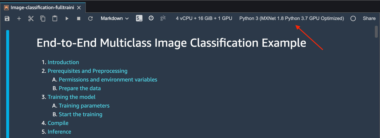
   Figure 7.20 – Choosing a kernel

7. Now, navigate through the code slowly. Please ensure you read the text preceding the code to better understand the functioning of each of these blocks.
8. Click the Run button, as highlighted in the following screenshot, to execute one block at a time. Please don't click on the Run button if you see an asterisk (*) adjacent to the block. The asterisk implies that the code is still running. Please wait for that to disappear before you proceed:
   

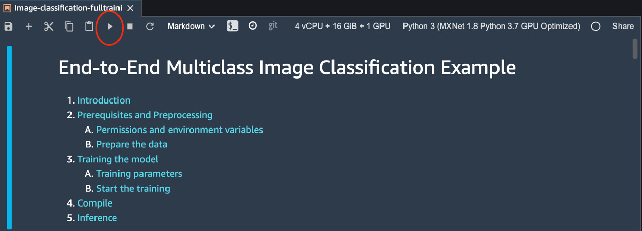
   Figure 7.21 – Running the steps

9. If you go through all the steps till the end, you will be able to complete the following steps:
   1. Downloading a training dataset
   2. Preparing and preprocessing the data
   3. Splitting the dataset into training and test samples
   4. Training the model using the appropriate framework and parameters
   5. Optimizing the model for the edge hardware
   6. Hosting the model artifacts on the Amazon S3 repository

   The model training can take up to 10 minutes to complete. After the training, you have an ML model that's trained using the MXNet framework and is capable of performing classification on 256 different objects.

10. Please navigate through the S3 bucket (sagemaker-<region>-<accountid>/ic-fulltraining/). Copy the S3 Uniform Resource Identifier (URI) for the model object (DLR-resnet50-*-cpu-ImageClassification.zip), as you will need it in the next section.

Now that the model is trained on the cloud, you will deploy it on the edge using Greengrass for near-real-time inferencing.

Deploying the model from cloud to the edge

As an IoT practitioner, deploying the model from the cloud to the edge is the step you will primarily be involved in. This is the transition point, where the ML or data science team provides a model that needs to be pushed to a fleet of devices on the edge. Although it's possible to automate these steps in the real world using a continuous integration/continuous deployment (CI/CD) pipeline, you will do it manually to learn the process in detail.

Similar to the components you have created in the earlier chapters for deploying different processes on the edge (such as publisher, subscriber, aggregator), deploying an ML resource needs the same approach. We will create a component that includes the ML model trained in the previous section. We will continue to use the AWS console for continuity.

Note

Greengrass provides a sample image classification model component that you toyed with in Chapter 4, Extending the Cloud to the Edge. Here, you are learning how to modify existing model components with your custom resources. In the real world, you may even have to create a new model component from scratch, where you can follow a similar process.

Let's begin. Proceed as follows:

1. Please navigate to the Amazon IoT Greengrass console, click on Components, click on the My components tab, and then on Create Component. Under Component information, select Enter recipe as JSON as your component source.

   In the Recipe box, paste the component recipe from the chapter7/recipe folder. Now, let's update the recipe to point to the trained model. Please replace the URI (marked with an arrow) with the S3 URI copied in Step 10 of the Building the ML workflow section, as illustrated in the following screenshot. If you have skipped the earlier section and used a trained model from GitHub, please manually upload the model to the S3 bucket of your choice and update the S3 URI in the recipe accordingly:

   

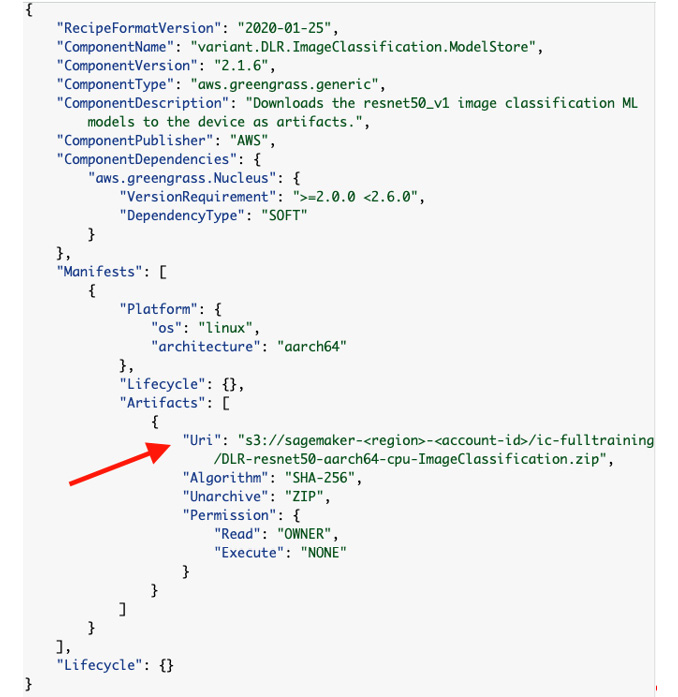
   Figure 7.22 – Recipe configuration

2. Click Create component to finish creating the model resource. This model should appear on the My components tab of the Components page.
3. Now, you need to create an inferencing component. This is the resource that triggers the model on the edge and publishes the results to the cloud.

   Note

   Greengrass provides a sample image classification inferencing component, aws.greengrass.DLRImageClassification, that you already played with in Chapter 4, Extending the Cloud to the Edge. Here, you are learning how to use the same inferencing component to work with your custom ML model. In the real world, you may have to create a new inferencing component from scratch with a modified manifest file, as you just did with the model.

4. On the Amazon Greengrass console, choose Deployments. On the Deployments page, revise your existing deployment and choose the following components:
   • variant.DLR.ImageClassification.ModelStore: ML model trained through SageMaker. You can choose this from the My components tab.
   • aws.greengrass.DLRImageClassification: Inferencing script for the ML model. You can choose this from the Public Component tab.
   • variant.DLR: Runtime required for the ML inferencing. You can choose this from the Public Component tab.
5. On the Select Components page, ensure the components shown in the following screenshot are chosen, and then click Next:
   

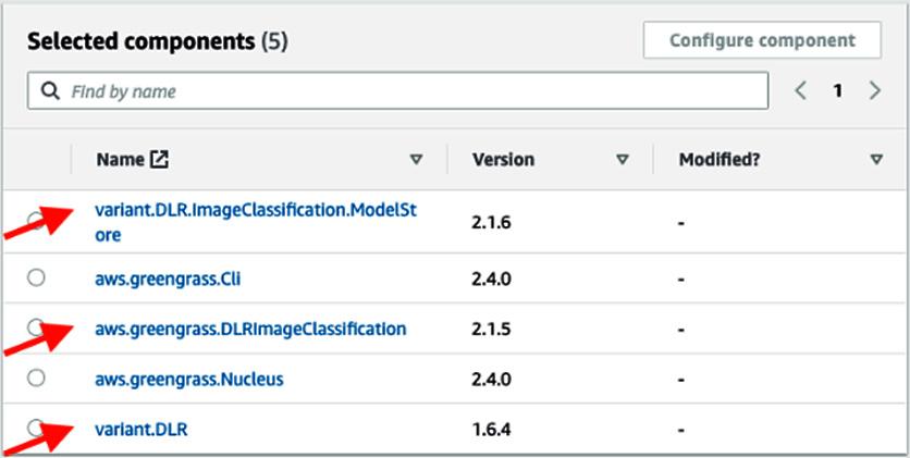
   Figure 7.23 – Greengrass component dependencies

6. On the Configure components page, select the aws.greengrass.DLRImageClassification component. This will enable the Configure component option; click on that.
7. Update the Configuration to merge section (right pane) with the following configuration and click on Confirm:

   {

     "InferenceInterval": "5"

   }

8. Keep all the other options as default in the following screens and choose Deploy.

Let's now move on to the next section.

Performing ML inferencing on the edge and validating results

So, by now, the models are built, trained, and deployed on Greengrass. The images to be inferred are stored in the following directory:

Figure 7.24 – Images directory on Greengrass hub

Similar to the cat image, you can deploy other images as well (such as dogs, humans, and so on) and configure the inferencing component to infer on them.

Let's visualize the inferencing results that are being published from the edge to the cloud. These results are key in assessing if the model is performing at the expected accuracy level. We'll proceed as follows:

1. First, let's check if the component status shows as running and also check the Greengrass log to verify that there are no exceptions. Here's the code we'll need to do this:

   sudo /greengrass/v2/bin/greengrass-cli component list

   sudo tail -100f /greengrass/v2/logs/greengrass.log

   sudo tail -100f aws.greengrass.DLRImageClassification.log

2. If there are no errors, please navigate to the AWS IoT console, choose Test, and then choose MQTT test client.
3. Under Subscriptions, choose ml/dlr/image-classification. Click Subscribe to view the results, which should look like this:

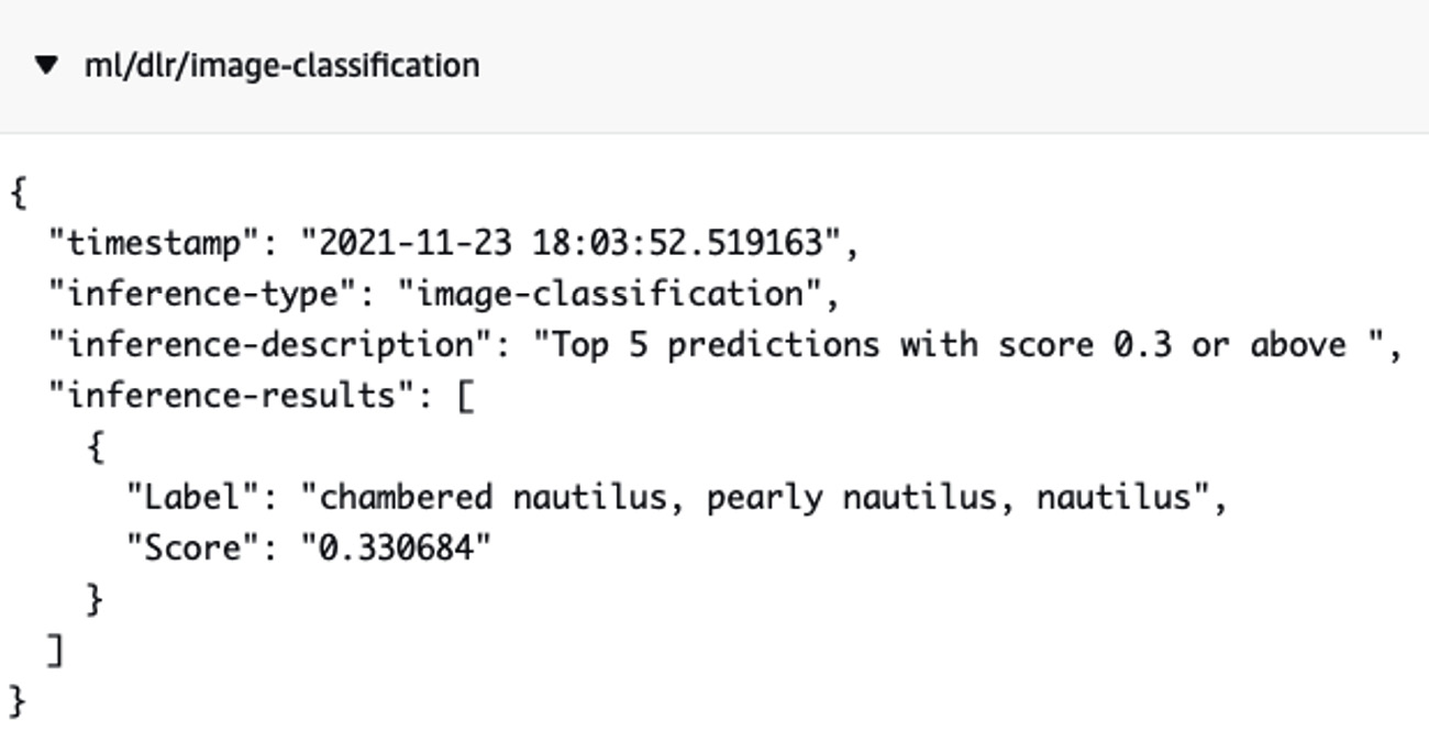
Figure 7.25 – Inferenced results from ML

If you get stuck or require help, please refer to the Troubleshooting section in GitHub.

Congratulations on finishing the hands-on section of this chapter! Now, your connected HBS hub is equipped with ML capabilities that can operate in both online and offline conditions and can classify humans, pets, and vehicles in your parking-space area.

Challenge Zone (Optional)

Can you figure out how to act on the inference results published to AWS IoT Core? This will be useful to automatically trigger an announcement through notifications/alarms for cautioning kids/pets strolling in the parking-space area.

Hint: You need to define a routing logic in the IoT Rules Engine to push the results through a notification service.

Isn't it incredible that you have now learned how to build ML capabilities for IoT workloads on the edge? It's time for a well-deserved break! Let's wrap up this chapter with a quick summary and a set of questions.

Summary

In this chapter, you were introduced to ML concepts relevant to IoT workloads. You learned how to design ML pipelines, along with optimizing models for IoT workloads. You implemented an edge-to-cloud architecture to perform inferences on unstructured data (images). Finally, you validated the workflow by visualizing the inferencing results from the edge for additional insights. 

In the next chapter, you will learn how to implement DevOps and MLOps practices to achieve operational efficiency for IoT edge workloads deployed at scale.

Knowledge check

Before moving on to the next chapter, test your knowledge by answering these questions. The answers can be found at the end of the book:

1. True or false: Two types of ML algorithms exist: supervised and unsupervised.
2. Can you recall the four types of ML systems and their significance?
3. True or false: K-means is a classification algorithm.
4. Can you put the three phases of the ML project life cycle in the right order?
5. Can you think of at least two common frameworks used for training ML models?
6. What is the AWS service used for deploying trained models from the cloud to the edge?
7. True or False: AWS IoT Greengrass only supports custom components for image classification problems.
8. Can you tell me about one anti-pattern for ML with IoT workloads?

References

Take a look at the following resources for additional information on the concepts discussed in this chapter:

• CRISP: https://www.datascience-pm.com/crisp-dm-2/
• A Short History of Machine Learning: https://www.forbes.com/sites/bernardmarr/2016/02/19/a-short-history-of-machine-learning-every-manager-should-read/?sh=1ca6cea115e7
• Machine Learning on AWS: https://aws.amazon.com/machine-learning/
• ML with AWS IoT services: https://aws.amazon.com/blogs/iot/category/artificial-intelligence/sagemaker/
• Using AWS IoT Greengrass Version 2 with Amazon SageMaker Neo and NVIDIA DeepStream Applications: https://aws.amazon.com/blogs/iot/using-aws-iot-greengrass-version-2-with-amazon-sagemaker-neo-and-nvidia-deepstream-applications/
• Well-Architected Framework for ML: https://docs.aws.amazon.com/wellarchitected/latest/machine-learning-lens/machine-learning-lens.html
• Learn from AWS through Machine Learning University (MLU): https://aws.amazon.com/machine-learning/mlu/