To illustrate this topic, we use a standard supply-versus-demand model from economics. In this model, supply and demand are related to prices by functional relationships, and the equilibrium market is found by determining the intersection of the supply and demand curves. The mathematical formulae we use in the example are somewhat arbitrary (thus possibly unrealistic) but will go beyond what is found in textbooks, where supply and demand are in general assumed to be linear.

The formulae that specify the supply and demand curves are as follows:

We will use the function factory pattern. Run the following lines of code in a cell:

def make_supply(A, B, C):
    def supply_func(q):
        return A * q / (C  - B * q)
    return supply_func
def make_demand(K, L):
    def demand_func(q):
        return K / (1 + L * q)
    return demand_func

The preceding code doesn't directly define the supply and demand curves. Instead, it specifies function factories. This approach makes it easier to work with parameters, which is what we normally want to do in applied problems since we expect the same model to be applicable to a variety of situations.

Next, we set the parameter values and call the function factories to define the functions that actually evaluate the supply and demand curves, as follows:

A, B, C = 23.3, 9.2, 82.4
K, L = 1.2, 0.54
supply = make_supply(A, B, C)
demand = make_demand(K, L)

The following lines of code make a graph of the curves:

q = linspace(0.01,5,200)
plot(q, supply(q), lw = 2)
plot(q, demand(q), lw = 2)
title('Supply and demand curves')
xlabel('Quantity (thousands of units)')
ylabel('Price ($)')
legend(['Supply', 'Demand'], loc='upper left')

The following is the graph that is the output of the preceding lines of code:

The curves chosen for supply and demand reflect what would be reasonable assumptions: supply increases and demand decreases as the price gets higher. Even with a zero price, the demand is finite (reflecting the fact that there is a limited population interested in the product). On the other hand, the supply curve has a vertical asymptote (not shown in the plot), indicating that there is a production limit (so, even if the price goes to infinity, there is a limited quantity that can be offered in the market).

The equilibrium point of the market is the intersection of the supply and demand curves. To find the equilibrium, we use the optimize module, which, besides providing functions for optimization, also has functions to solve numerical equations. The recommended function to find solutions for one-variable functions is brentq(), as illustrated in the following code:

from scipy import optimize
def opt_func(q):
    return supply(q) - demand(q)
q_eq = optimize.brentq(opt_func, 1.0, 2.0)
print q_eq, supply(q_eq), demand(q_eq)

The brentq() function assumes that the right-hand side of the equation we want to solve is 0. So, we start by defining the opt_func() function that computes the difference between supply and demand. This function is the first argument of brentq(). The next two numerical arguments give an interval that contains the solutions. It is important to choose an interval that contains exactly one solution of the equation. In our example, this is easily done by looking at the graph, from which it is clear that the curves intersect between 1 and 2.

Running the preceding code produces the following output:

1.75322153719 0.616415252177 0.616415252177

The first value is the equilibrium point, which is the number of units (in thousands) that can be sold at the optimal price. The optimal price is computed using both the supply and demand curves (to check that the values are indeed the same).

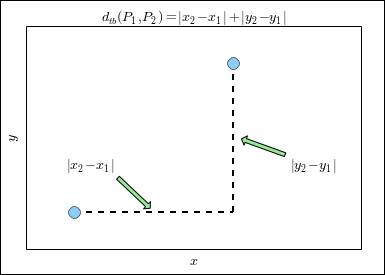
To illustrate an optimization problem in two variables, let's consider a problem of optimal facility location. Suppose a factory has several manufacturing stations that need materials to be distributed from a single supply station. The factory floor is rectangular, and the distribution rails must be parallel to the walls of the factory. This last requirement is what makes the problem interesting. The function to be minimized is related to the so-called taxicab distance, which is illustrated in the following image:

The first step is to define the points where the manufacturing stations are given, as follows:

points = array([[10.3,15.4],[6.5,8.8],[15.6,10.3],[4.7,12.8]])

The positions are stored as a 4 x 2 NumPy array called points, with one point in each row. The following command produces a plot of the points mentioned in the previous command line:

plot(points[:,0],points[:,1], 'o', ms=12, mfc='LightSkyBlue')

The points are displayed using a circular marker specified by the argument o, which also turns off the line segments connecting the points. The ms and mfc options specify the size of the marker (in pixels) and its color, respectively. The following image is then generated as the output:

The next step is to define the function to be minimized. We again prefer the approach of defining a function factory, as follows:

def make_txmin(points):
    def txmin_func(p):
        return sum(abs(points - p))
    return txmin_func

The main point of this code is the way in which the taxicab distance is computed, which takes full advantage of the flexibility of the array operations of NumPy. This is done in the following line of code:

return sum(abs(points - p))

This code first computes the vector difference, points-p. Note that, here, points is a 4 x 2 array, while p is a 1 x 2 array. NumPy realizes that the dimensions of the arrays are different and uses its broadcasting rules. The effect is that the array p is subtracted from each row of the points array, which is exactly what we want. Then the abs() function computes the absolute value of each of the entries of the resulting array, and finally sum() adds all the entries. That's a lot of work done in a single line of code!

We then have to use the function factory to define the function that will actually compute the taxicab distance.

txmin = make_txmin(points)

The function factory is simply called with the array containing the actual positions as its argument. At this point, the problem is completely set up, and we are ready to compute the optimum, which is done with the following code:

from scipy import optimize
x0 = array([0.,0.])
res = optimize.minimize(
         txmin, x0,
         method='nelder-mead',
         options={'xtol':1e-5, 'disp':True})

The minimization is computed by a call to the minimize() function. The first two arguments of this function are the objective function defined in the previous cell, txmin(), and an initial guess, x0. We just choose the origin as the initial guess, but in a real-world problem, we use any information we can gather to select a guess that is close to the actual minimum. Several optimization methods are available, suitable for different types of objective functions. We use the Nelder-Mead method, which is a heuristic algorithm that does not require smoothness of the objective function. This is well suited for the problem at hand. Finally, we specify two options for the method: the desired tolerance and a display option to print diagnostics. This produces the following output:

Optimization terminated successfully.
         Current function value: 23.800000
         Iterations: 87
         Function evaluations: 194

The preceding output states that a minimum was successfully found and gives its value. Note that, as in any numerical optimization method, in general, it can only be guaranteed that a local minimum was found. In this case, since the objective function is convex, the minimum is guaranteed to be global. The result of the function is stored in a SciPy data structure of the OptimizeResult type defined in the optimize module. To get the optimal position of the facility, we can use the following command:

print res.x

The output of the preceding command is as follows:

[  8.37782286  11.36247412]

To finish this example, we present the code that displays the optimal solution:

plot(points[:,0],points[:,1], 'o', ms=12, mfc='LightSkyBlue')
plot(res.x[0], res.x[1],'o', ms=12, mfc='LightYellow')
locstr = 'x={:5.2f}, y={:5.2f}'.format(res.x[0], res.x[1])
title('Optimal facility location: {}'.format(locstr))

The calls to the plot() function are similar to the ones in the previous example. To give a nicely formatted title, we first define the locstr string, which displays the optimal location coordinates. This is a Python-formatted string with the format specification of {:5.2f}, that is, a floating-point field with width 5 and a precision of 2 digits. The result is the following figure:

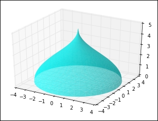
As an example of a calculus computation, we will show you how to compute the volume of a solid of revolution. The solid is created by rotating the curve displayed in the following figure around the y-axis:

This curve is plotted with the following code:

def make_gen(a,b):
    def gen_func(y):
        return a/pi * arccos(2.0 * y / b - 1.0)
    return gen_func
a = 5.
b = 4.
gen = make_gen(a,b)
x = linspace(0,b,200)
y = gen(x)
subplot(111, aspect='equal')
plot(x,y,lw=2)

The curve is essentially a stretched and transposed inverse cosine function, as defined in the make_gen() function. It depends on two parameters, a and b, that specify its height and length, respectively. The make_gen() function is a function factory that returns a function that actually computes values in the curve. The actual function defining the curve is called gen() (for generator), so this is the function that is plotted.

When this curve is rotated around the vertical axis, we obtain the solid plotted as follows:

The preceding figure, of course, was generated with IPython using the following code:

from mpl_toolkits.mplot3d import Axes3D
na = 50
nr = 50
avalues = linspace(0, 2*pi, na, endpoint=False)
rvalues = linspace(b/nr, b, nr)
avalues_r = repeat(avalues[...,newaxis], nr, axis=1)
xvalues = append(0, (rvalues*cos(avalues_r)).flatten())
yvalues = append(0, (rvalues*sin(avalues_r)).flatten())
zvalues = gen(sqrt(xvalues*xvalues+yvalues*yvalues))
fig = plt.figure()
ax = fig.gca(projection='3d')
ax.plot_trisurf(xvalues, yvalues, zvalues, 
                color='Cyan',alpha=0.65,linewidth=0.)

The key function in this code is the call to plot_trisurf() in the last line. This function accepts three NumPy arrays, xvalues, yvalues, and zvalues, specifying the coordinates of the points on the surface. The arrays, xvalues and yvalues define points in a succession of concentric circles, as shown in the following image:

The value of the z coordinate is obtained by computing gen(sqrt(x*x+y*y)) at each of these points, which has the effect of assigning the same height in the 3D plot to all points of each concentric circle.

To compute the volume of the solid, we use the method of cylindrical shells. An explanation of how the method works is beyond the scope of this book, but it boils down to computing an integral, as shown in the following formula:

In this formula, the f(x) function represents the curve being rotated around the y-axis. To compute this integral, we use the scipy.integrate package. We use the quad() function, which is appropriate for the generic integration of functions that do not have singularities. The following is the code for this formula:

import scipy.integrate as integrate
int_func  = lambda x: 2 * pi * x * gen(x)
integrate.quad(int_func, 0, b)

After importing the integrate module, we define the function to be integrated. Note that we use the lambda syntax since this is a one-line calculation. Finally, we call quad() to perform the integration. The arguments to the call are the function being integrated and the bounds of integration (from 0 to b in this case). The following is the output of the preceding lines of code:

(94.24777961000055, 1.440860870616234e-07)

The first number is the value of the integral, and the second one is an error estimate.

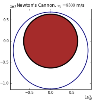
In the next example, we consider Newton's canon, a thought experiment at the very root of modern physics and calculus. The situation is illustrated in the following image, which is an engraving from the book by Sir Isaac Newton, A Treatise of The System of the World:

Newton asks us to imagine a canon sitting at the top of a very high mountain. If the canon shoots a projectile, it will fly for a while and eventually hit the ground. The larger the initial velocity of the projectile, the further away it will hit the ground. Let's imagine that we can shoot the projectile as fast as we want, and that there is no air resistance. Then, as the initial velocity increases, eventually the projectile will go around the earth and, if the canon is removed quickly enough, then the projectile will continue its orbit around Earth forever. Newton used this example to explain how the moon could revolve around Earth without ever falling under the action of gravity alone.

To model this situation, we need to use Newton's law of gravitation as a system of differential equations:

We will not attempt to explain how these formulae were obtained, with the only important point for us being that there are four state variables, with the first two representing the position of the projectile and the last two representing its velocity vector. Since the movement takes place in a plane through the center of Earth, only two position variables are needed. G and M are constants representing Newton's universal gravitational constant and the mass of Earth, respectively. The mass of the projectile does not appear, since the gravitational mass is exactly cancelled by the inertial mass.

The first step to solve this using SciPy is to define this set of differential equations, which is done with the following code:

M = 5.9726E24
G = 6.67384E-11
C = G * M
def ode_func(xvec, t):
    x1, x2, v1, v2 = xvec
    d = (x1 * x1 + x2 * x2) ** 1.5
    return array([v1, v2, -C * x1 / d, -C * x2 / d ])

All that we need to do is define a function that computes the right-hand side of the system of differential equations. We start by defining the constants, M and G (using SI units), and the auxiliary constant C, since G and M only appear in the equations through their product. The system is represented by the ode_func() function. This function must accept at least two parameters: a NumPy array, xvec, and a floating-point value, t. In our case, xvec is a four-dimensional vector since there are four state variables in our system. The variable, t, is not used in the system since there are no external forces (as there would be if we were launching a rocket instead of shooting a projectile). However, it must still be listed as an input parameter.

Inside ode_func(), we first extract the elements of the xvec vector with the assignment, as follows:

x1, x2, v1, v2 = xvec

This is not strictly necessary but improves readability. We then compute the auxiliary quantity, d (this is the denominator of the last two equations). Finally, the output array is computed according to the formulae in the system. Note that no derivatives are computed since all information that is needed by the solver is contained in the right-hand side of the equations.

We are now ready to solve the system of differential equations using the following lines of code:

import scipy.integrate as integrate
earth_radius = 6.371E6
v0 = 8500
h0 = 5E5
ic = array([0.0, earth_radius + h0, v0, 0.0])
tmax = 8700.0
dt = 10.0
tvalues = arange(0.0, tmax, dt)
xsol = integrate.odeint(ode_func, ic, tvalues)

The first line of the preceding code imports the integrate module, where the differential equations are solved. We then need to specify the initial position and velocity of the projectile. We assume that the canon is at the North Pole, atop a tower of 50,000 m (although this is clearly unrealistic, we just choose such a large value to enhance the visibility of the orbit). Since Earth is not a perfect sphere, we use an average value for the radius. The initial velocity is set to 8500 m/s.

The initial conditions are stored in a NumPy array with the following assignment:

ic = array([0.0, earth_radius + h0, v0, 0.0])

The next step is to define the initial time (zero in our case) and the array of times at which the solution is sought. This is done with the following three lines of code:

tmax = 8650.0
dt = 60.0
tvalues = arange(0.0, tmax, dt)

We first define tmax as being the duration of the simulation (in seconds). The variable dt stores the time intervals at which we want to record the solution. In the preceding code, the solution will be recorded every 60 seconds for 8,650 seconds. The final time was chosen by trial-and-error to correspond, approximately, to one orbit of the projectile.

We are now ready to compute the solution, which is done with a call to the odeint() function. The solution is stored in the vector, xsol, which has one row for each time at which the solution is computed. To see the first few rows of the vector, we can run the following command:

xsol[:10]

The preceding command produces the following output:

array([[  0.00000000e+00,   6.87100000e+06,   8.50000000e+03,
          0.00000000e+00],
       [  5.09624253e+05,   6.85581217e+06,   8.48122162e+03,
         -5.05935282e+02],
       [  1.01700042e+06,   6.81036510e+06,   8.42515172e+03,
         -1.00800330e+03],
       [  1.51991202e+06,   6.73500470e+06,   8.33257580e+03,
         -1.50243025e+03],
       [  2.01620463e+06,   6.63029830e+06,   8.20477026e+03,
         -1.98562415e+03],
       [  2.50381401e+06,   6.49702131e+06,   8.04345585e+03,
         -2.45425372e+03],
       [  2.98079103e+06,   6.33613950e+06,   7.85073707e+03,
         -2.90531389e+03],
       [  3.44532256e+06,   6.14878788e+06,   7.62903174e+03,
         -3.33617549e+03],
       [  3.89574810e+06,   5.93624710e+06,   7.38099497e+03,
         -3.74461812e+03],
       [  4.33057158e+06,   5.69991830e+06,   7.10944180e+03,
         -4.12884566e+03]])

These values are the position and velocity vectors of the projectile from time 0 s to time 360 s at intervals of 60 s.

We definitely want to produce a plot of the orbit. This can be done by running the following code in a cell:

subplot(111, aspect='equal')
axis(earth_radius * array([-1.5, 1.5, -1.8, 1.2]))
earth = Circle((0.,0.), 
                earth_radius, 
                ec='Black', fc='Brown', lw=3)
gca().add_artist(earth)
plot(xsol[:,0], xsol[:,1], lw=2, color='DarkBlue')
title('Newton's Canon, $v_0={}$ m/s'.format(v0))

We want to use the same scale in both axes since both axes represent spatial coordinates in meters. This is done in the first line of code. The second line sets the axis limits so that the plot of the orbit fits comfortably in the picture.

Then, we plot a circle to represent Earth using the following lines of code:

earth = Circle((0.,0.), 
               earth_radius, 
               ec='Black', fc='Brown', lw=3)
gca().add_artist(earth)

We have not emphasized using Artist objects in our plots since these are at a lower level than is usually required for scientific plots. Here, we are constructing a Circle object by giving its center, radius, and appearance options: a black edge color, brown face color, and a line width equal to 3. The second line of code shows how to add the Circle object to the plot.

After drawing Earth, we plot the orbit using the following line of code:

plot(xsol[:,0], xsol[:,1], lw=2, color='DarkBlue')

This is a standard call to the plot() function. Note that we plot only the first two columns of the xsol array since these represent the position of the projectile (recall that the other two represent the velocity). The following image is what we get as the output:

A numerical solution for differential equations is a sophisticated topic, and a complete treatment of the issue is beyond the scope of this book, but we will present the full form of the odeint() function and comment on some of the options. The odeint() function is a Python wrapper on the lsoda solver from ODEPACK, the Fortran library. Detailed information about the solver can be found at http://people.sc.fsu.edu/~jburkardt/f77_src/odepack/odepack.html

The following lines of code are the complete signature of odeint():

odeint(ode_func, x0, tvalues, args=(), Dfun=None, col_deriv=0,
       full_output=0, ml=None, mu=None, rtol=None, atol=None,
       tcrit=None, h0=0.0, hmax=0.0, hmin=0.0,ixpr=0, mxstep=0,
       mxhnil=0, mxordn=12, mxords=5, printmessg=0)

The arguments, ode_func, x0 and tvalues, have already been discussed. The argument args allows us to pass extra parameters to the equation being solved. This is a very common situation, which is illustrated in the next example. In this case, the function defining the system must have the following signature:

ode_func(x, t, p1, p2, … , pn)

Here, p1, p2, and pn are extra parameters. These parameters are fixed for a single solution but can change from one solution to the other (they are normally used to represent the environment). The tuple passed to args must have a length exactly equal to the number of parameters that ode_func() requires.

The following is a partial list of the meaning of the most common options:

In the last example in this section, we present the Lorenz oscillator, a simplified model for atmospheric convection, and a famous equation that displays chaotic behavior for certain values of the parameters. We will also use this example to demonstrate how to plot solutions in three dimensions.

The Lorenz system is defined by the following equations:

We start by defining a Python function representing the system, as follows:

def ode_func(xvec, t, sigma, rho, beta):
    x, y, z = xvec
    return array([sigma * (y - x),
                  x * (rho - z) - y,
                  x * y - beta * z ])

The only difference between this system and the previous one is the presence of the parameters sigma, rho, and beta. Note that they are just added as extra arguments to ode_func(). Solving the equation is almost the same as solving the previous example:

tmax = 50
tdelta = 0.005
tvalues = arange(0, tmax, tdelta) 
ic = array([0.0, 1.0, 0.0])
sol = integrate.odeint(ode_func, ic, tvalues, 
                       args=(10., 28., 8./3.))

We define the array of times and the initial condition just as we did in the previous example. Notice that since this is a three-dimensional problem, there are initial conditions in an array with three components. Then comes the call to odeint(). The call now has an extra argument:

args=(10., 28., 8./3.)

This sets sigma, rho, and beta, respectively, to the values 10, 28, and 8/3. These are values that are known to correspond to chaotic solutions.

The solution can then be plotted with the following code:

from mpl_toolkits.mplot3d import Axes3D
fig = plt.figure(figsize=(8,8))
from mpl_toolkits.mplot3d import Axes3D
fig = plt.figure(figsize=(8,8))
ax = fig.add_subplot(111, projection='3d')
x, y, z = sol.transpose() 
ax.plot(x, y, z, lw=0.5, color='DarkBlue')
ax.set_xlabel('$x$')
ax.set_ylabel('$y$')
ax.set_zlabel('$z$')

The first three lines of code set up the axes for three-dimensional plotting. The next line extracts the data in a format suitable for plotting:

x, y, z = sol.transpose()

This code illustrates a common pattern. The array sol contains the coordinates of the solutions along its columns, so we transpose the array so that the data is along the rows of the array, and then assign each row to one of the variables x, y, and z.

The other lines of code are pretty straightforward: we call the plot() function and then add labels to the axes. The following is the figure that we get as the output:

The preceding image is known as the classical Lorenz butterfly, a striking example of a strange attractor.