When working with projects of some complexity, it is common to have the need to run scripts written by others. It is also always necessary to load data and save results. In this section, we will describe the facilities that IPython provides for these tasks.
The following Python script generates a plot of a solution of the Lorenz equations, a famous example in the theory of chaos. If you are typing the code, do not type it in a cell in the notebook. Instead, use a text editor and save the file with the name lorenz.py in the same directory that contains the notebook file. The code is as follows:
import numpy as np
import matplotlib.pyplot as plt
from scipy.integrate import odeint
from mpl_toolkits.mplot3d import Axes3D

def make_lorenz(sigma, r, b):
    def func(statevec, t):
        x, y, z = statevec
        return [ sigma * (y - x),
                 r * x - y - x * z,
                 x * y - b * z ]
    return func

lorenz_eq = make_lorenz(10., 28., 8./3.)

tmax = 50
tdelta = 0.005
tvalues = np.arange(0, tmax, tdelta)
ic = np.array([0.0, 1.0, 0.0])
sol = odeint(lorenz_eq, ic, tvalues)

x, y, z = np.array(zip(*sol))

fig = plt.figure(figsize=(10,10))
ax = fig.add_subplot(111, projection='3d')
ax.plot(x, y, z, lw=1, color='red')
ax.set_xlabel('$x$')
ax.set_ylabel('$y$')
ax.set_zlabel('$z$')
plt.show()
Now, go to the notebook and run a cell using the following command:
%run lorenz.py
This will run the script and produce a plot of the solution, as shown in the following figure:
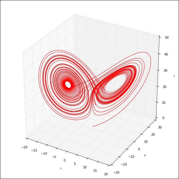
The %run magic executes the script in the notebook's namespace so that all global variables, functions, and classes defined in the script are made available in the current notebook.
It is also possible to use the %load magic for the same purpose:
%load lorenz.py
The difference is that %load does not immediately run the script, but places its code in a cell. It can then be run from the cell it was inserted in. A slightly annoying behavior of the %load magic is that it inserts a new cell with the script code even if there already is one from a previous use of %load. The notebook has no way of knowing if the user wants to overwrite the code in the existing cell, so this is the safest behavior. However, unwanted code must be deleted manually.
The %load magic also allows code to be loaded directly from the web by providing a URL as input:
%load http://matplotlib.org/mpl_examples/pylab_examples/boxplot_demo2.py
This will load the code for a box plot example from the matplotlib site to a cell. To display the image, the script must be run in the cell.
We can also run scripts written in other languages directly in the notebook. The following table contains some of the supported languages:
Now, let's see some examples of scripts in some of these languages. Run the following code in a cell:
%%SVG
<svg width="400" height="300">
    <circle  cx="200" cy="150" r="100"
        style="fill:Wheat; stroke:SteelBlue; stroke-width:5;"/>
    <line x1="10" y1="10" x2="250" y2="85"
        style="stroke:SlateBlue; stroke-width:4"/>
    <polyline points="20,30 50,70 100,25 200,120"
        style="stroke:orange; stroke-width:3;
               fill:olive; opacity:0.65;"/>
    <rect x="30" y="150" width="120" height="75"
        style="stroke:Navy; stroke-width:4; fill:LightSkyBlue;"/>
    <ellipse cx="310" cy="220" rx="55" ry="75"
        style="stroke:DarkSlateBlue; stroke-width:4;
               fill:DarkOrange; fill-opacity:0.45;"/>
    <polygon points="50,50 15,100 75,200 45,100"
        style="stroke:DarkTurquoise; stroke-width:5; fill:Beige;"/>
</svg>
This displays a graphic composition with basic shapes, described using SVG. SVG is an HTML standard, so this code will run in modern browsers that support the standard.
To illustrate the use of JavaScript, let's first define (in a computation cell) an HTML element that can be easily accessed:
%%html
<h1 id="hellodisplay">Hello, world!</h1>
Run this cell. The message "Hello, world!" in the size h1 is displayed. Then enter the following commands in another cell:
%%javascript
element = document.getElementById("hellodisplay")
element.style.color = 'blue'
When the second cell is run, the color of the text of the "Hello, world!" message changes from black to blue.
The notebook can actually run any scripting language that is installed in your system. This is done using the %%script cell magic. As an example, let's run some code in the Julia scripting language. Julia is a new language for technical computing and can be downloaded from http://julialang.org/. The following example assumes that Julia is installed and can be accessed with the julia command (this requires that the executable for the language interpreter is in the operating system's path). Enter the following code in a cell and run it:
%%script julia
function factorial(n::Int)
    fact = 1
    for k=1:n
      fact *= k
    end
    fact
end

println(factorial(10))
The preceding code defines a function (written in julia) that computes the factorial of an integer, and then prints the factorial of 10. The following output is produced:
factorial (generic function with 1 method)
3628800
The first line is a message from the julia interpreter and the second is the factorial of 10.
The manner in which data is loaded or saved is dependent on both the nature of the data and the format expected by the application that is using the data. Since it's impossible to account for all combinations of data structure and application, we will only cover the most basic methods of loading and saving data using NumPy in this section. The recommended way to load and save structured data in Python is to use specialized libraries that have been optimized for each particular data type. When working with tabular data, for example, we can use pandas, as described in Chapter 4, Handling Data with pandas.
A single array can be saved with a call to the save() function of NumPy. Here is an example:
A = rand(5, 10)
print A
save('random_array.npy', A)
This code generates an array of random values with five rows and 10 columns, prints it, and then saves it to a file named random_array.npy. The .npy format is specific for NumPy arrays. Let's now delete the variable containing the array using the following command:
del A
A
Running a cell with the preceding commands will produce an error, since we request the variable A to be displayed after it has been deleted. To restore the array, run the following command in a cell:
A = load('random_array.npy')
A
It is also possible to save several arrays to a single compressed file, as shown in the following example:
xvalues = arange(0.0, 10.0, 0.5)
xsquares = xvalues ** 2
print xvalues
print xsquares
savez('values_and_squares.npz', values=xvalues, squares=xsquares)
Notice how keyword arguments are given to specify names for the saved arrays in disk. The arrays are now saved to a file in the .npz format. The data can be recovered from disk using the load() function, which can read files in both formats used by NumPy:
my_data = load('values_and_squares.npz')
If the file passed to load() is of the .npz type, the returned value is an object of the NpzFile type. This object does not read the data immediately. Reading is delayed to the point where the data is required. To figure out which arrays are stored in the file, execute the following command in a cell:
my_data.files
In our example, the preceding command produces the following output:
['squares', 'values']
To assign the arrays to variables, use the Python dictionary access notation as follows:
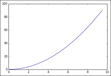
xvalues = my_data['values']
xsquares = my_data['squares']
plot(xvalues, xsquares)
The preceding code produces the plot of half of a parabola: