In this section, we will work with a realistic dataset of moderate size. We will use the World Development Indicators dataset, which is provided free of charge by the World Bank. This is a reasonably sized dataset that is not too large or complex to experiment with.

In any real application, we will need to read data from some source, reformat it to our purposes, and save the reformatted data back to some storage system. pandas offers facilities for data retrieval and storage in multiple formats:

The list of formats supported by pandas keeps growing with each new update to the library. Please refer to http://pandas.pydata.org/pandas-docs/stable/io.html for a current list.

Treating all formats supported by pandas is not possible in a book with the current scope. We will restrict examples to CSV files, which is a simple text format that is widely used. Most software packages and data sources have options to format data as CSV files.

Curiously enough, CSV is not a formally described storage format. pandas does a good job of providing enough options to read the great majority of files. However, the format of the data may vary depending on the data source. Luckily, since CSV files are simply text files, we can open the files in a spreadsheet program or even a text editor to examine their structure.

The dataset for this section can be downloaded from http://data.worldbank.org/data-catalog/world-development-indicators, and is also available in the book website. If you choose to download the data from the original website, make sure you choose the CSV file format. The file is in compressed ZIP format, and is about 40 MB in size. Once the archive is decompressed, we get the following files.

As is typical of any realistic dataset, there's always a lot of ancillary information associated with the data. This is called metadata and is used to give information about the dataset, including things such as the labels used for rows and/or columns, data collection details, and explanations concerning the meaning of the data. The metadata is contained in the various files contained within the archive. The reader is encouraged to open the different files using spreadsheet software (or a text editor) to get a feel for the kind of information available. For us, the most important metadata file is WDI_Series.csv, which contains information on the meaning of data labels for the several time series contained in the data.

The actual data is in the WDI_Data.csv file. As this file contains some of the metadata information, we will be able to do all the work using this file only.

Make sure the WDI_Data.csv file is in the same directory that contains your IPython notebook files, and run the following command in a cell:

wdi = pd.read_csv('WDI_Data.csv')

This will read the file and store it in a DataFrame object that we assign to the variable, wdi. The first row in the file is assumed to contain the column labels by default. We can see the beginning of the table by running the following command:

wdi.loc[:5]

Note that the DataFrame class is indexed by integers by default. It is possible to choose one of the columns in the data file as the index by passing the index_col parameter to the read_csv() method. The index column can be specified either by its position or by its label in the file. The many options available to read_csv() are discussed in detail at http://pandas.pydata.org/pandas-docs/stable/io.html#io-read-csv-table.

An examination of the file shows that it will need some work to be put in a format that can be easily used. Each row of the file contains a time series of annual data corresponding to one country and economic indicator. One initial step is to get all the countries and economic indicators contained in the file. To get a list of unique country names, we can use the following command line:

countries = wdi.loc[:,'Country Name'].unique()

To see how many countries are represented, run the following command line:

len(countries)

Some of the entries in the file actually correspond to groups of countries, such as Sub-Saharan Africa.

Now, for indicators, we can run the following command line:

indicators = wdi.loc[:,'Indicator Code'].unique()

There are more than 1300 different economic indicators in the file. This can be verified by running the following command line:

len(indicators)

To show the different kinds of computation one might be interested in performing, let's consider a single country, for example, Brazil. Let's also suppose that we are only interested on the Gross Domestic Product (GDP) information. Now, we'll see how to select the data we are interested in from the table. To make the example simpler, we will perform the selection in two steps. First, we select all rows for the country name Brazil, using the following command line:

wdi_br = wdi.loc[wdi.loc[:,'Country Name']=='Brazil',:]

In the code preceding command line, consider the following expression:

wdi.loc[:,'Country Name']=='Brazil'

This selects all the rows in which the country name string is equal to Brazil. For these rows, we want to select all columns of the table, as indicated by the colon in the first term of the slicing operation.

Let's now select all the rows that refer to the GDP data. We start by defining a function that, given a string, determines if it contains the substring GDP (ignoring the case):

select_fcn = lambda string: string.upper().find('GDP') >= 0

We now want to select the rows in wdi_br that return True when select_fcn is applied to the Indicator Code column. This can be done with the following command lines:

criterion = wdi_br.loc[:,'Indicator Code'].map(select_fcn)
wdi_br_gdp = wdi_br.loc[criterion,:]

The map() method of the Series object does exactly what we want: it applies a function to all elements of a series. We assign the result of this call to the variable, criterion. Then, we use criterion in the slicing operation that defines wdi_br_gdp. To see how many rows were selected, run the following command:

len(wdi_br_gdp)

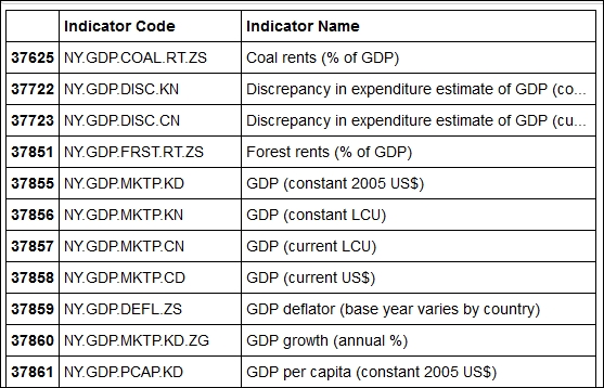
In the dataset used at the writing of this book, the preceding command returns 32. This means that there are 32 GDP-related indicators for the country named Brazil. Since we now have a manageable amount of data, we can display a table that has the indicator codes and their meanings using the following command line:

wdi_br_gdp.loc[:,['Indicator Code', 'Indicator Name']]

The preceding command line generates a nicely formatted table of the indicator and corresponding names, as shown in the following table:

Let's say that we are interested only in four indicators: the GDP, annual GDP growth, GDP per capita, and GDP per capita growth. We can further trim the data with the following command:

wdi_br_gdp = wdi_br_gdp.loc[[37858, 37860, 37864, 37865], :]

This produces quite a manageable table with 4 rows and 58 columns. Each row contains a time series of the corresponding GDP data starting with the year 1960.

The problem with this table as it is laid out is that it is the "transpose" of what is the usual convention in pandas: the time series are across the rows of the table, instead of being down the columns. So, we still need to do a little more work with our table. We want the indexes of our table to be the years. We also want to have one column for each economic indicator and want to use the economic indicator names (not the codes) as the labels of the columns. Here is how this can be done:

idx = wdi_br_gdp.loc[:,'1960':].columns
cols = wdi_br_gdp.loc[:,'Indicator Name']
data = wdi_br_gdp.loc[:,'1960':].as_matrix()
br_data = DataFrame(data.transpose(), columns=cols, index=idx)

The following is an explanation of what the preceding command lines do:

Now that we have the data we want in a nice format, it is a good time to save it:

br_data.to_csv('WDI_Brazil_GDP.csv')

At this point, we can open the WDI_Brazil_GDP.csv file in a spreadsheet program to view it.

Now, let's start playing with the data by creating a few plots. Let's first plot the GDP and GDP growth, starting in 1980. Since the data is given in dollars, we scale to give values in billions of dollars.

pdata = br_data.ix['1970':, 0] / 1E9
pdata.plot(color='DarkRed', lw=2, 
           title='Brazil GDP, billions of current US$')

The preceding command lines produce the following chart:

As a final example, let's draw a chart comparing the percent growth of per capita GDP for the BRIC (Brazil, Russia, India, and China) countries in the period 2000 to 2010. Since we already have explored the structure of the data, the task is somewhat simpler:

bric_countries = ['Brazil', 'China', 'India', 'Russian Federation']
gdp_code = 'NY.GDP.PCAP.KD.ZG'
selection_fct = lambda s: s in bric_countries
criterion = wdi.loc[:,'Country Name'].map(selection_fct)
wdi_bric = wdi.loc[criterion & (wdi.loc[:,'Indicator Code'] == gdp_code),:]

We first define a list with the names of the BRIC countries and a string with the indicator code for percent GDP growth per capita. Then, we define a selection function: a string is selected if it is one of the BRIC country names. The map() method is then used to apply the selection function to all entries of the Country Name column. The last command line performs the actual selection. Note the use of the Boolean operator & to combine the two criteria used in the row selection.

We now perform the reformatting of the data to have the relevant data series along the columns of the table. The command lines are similar to the ones in the previous example:

df_temp = wdi_bric.loc[:, '2000':'2010']
idx = df_temp.columns
cols = wdi_bric.loc[:, 'Country Name']
data = df_temp.as_matrix()
bric_gdp = DataFrame(data.transpose(), columns=cols, index=idx)

Once this is done, plotting the data is straightforward:

bric_gdp.plot(lw=2.5,
              title='Annual per capita GDP growth (%)')

The preceding command lines result in the following plot: