The DataFrame class is used to represent two-dimensional data. To illustrate its use, let's create a DataFrame class containing student data as follows:

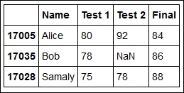
grades = DataFrame(
    [['Alice',  80., 92., 84,],
     ['Bob',    78., NaN, 86,],
     ['Samaly', 75., 78., 88.]],
    index = [17005, 17035, 17028],
    columns = ['Name', 'Test 1', 'Test 2', 'Final']
    )

This code demonstrates one of the most straightforward ways to construct a DataFrame class. In the preceding case, the data can be specified as any two-dimensional Python data structure, such as a list of lists (as shown in the example) or a NumPy array. The index option sets the row names, which are integers representing student IDs here. Likewise, the columns option sets the column names. Both the index and column arguments can be given as any one-dimensional Python structure, such as lists, NumPy arrays, or a Series object.

To display the output of the DataFrame class, run the following statement in a cell:

grades

The preceding command displays a nicely formatted table as follows:

The DataFrame class features an extremely flexible interface for initialization. We suggest that the reader run the following command to know more about it:

DataFrame?

This will display information about the construction options. Our goal here is not to cover all possibilities, but to give an idea of the offered flexibility. Run the following code in a cell:

idx = pd.Index(["First row", "Second row"])
col1 = Series([1, 2], index=idx)
col2 = Series([3, 4], index=idx)
data = {"Column 1":col1, "Column2":col2}
df = DataFrame(data)
df

The preceding code produces the following table:

This example illustrates a useful way of thinking of a DataFrame object: it consists of a dictionary of Series objects with a common Index object labeling the rows of the table. Each element in the dictionary corresponds to a column in the table. Keep in mind that this is simply a way to conceptualize a DataFrame object, and this is not a description of its internal storage.

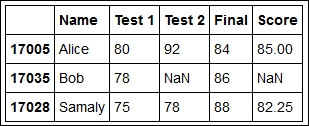
Let's go back to our student data example. Let's add a column with the total score of each student, which is the average of the grades, with the final having weight two. This can be computed with the following code:

grades.loc[:,'Score'] = 0.25 * (grades['Test 1'] + grades['Test 2'] + 2 * grades['Final']) 
grades

The output for the preceding command line is as follows:

In the preceding command line, we used one of the following recommended methods of accessing elements from a DataFrame class:

To use any of these methods, the corresponding entry (or entries) in the DataFrame object must already exist. So, these methods cannot be used to insert or append new data.

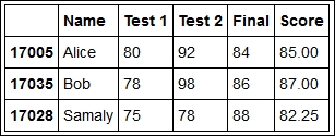
Notice that Bob does not have a grade in his second test, indicated by the NaN entry (he was probably sick on the day of the test). When he takes a retest, his grade can be updated as follows:

grades.loc[17035,'Test 2'] = 98
grades

In the output, you will notice that Bob's final score is not automatically updated. This is no surprise because a DataFrame object is not designed to work as a spreadsheet program. To perform the update, you must explicitly execute the cell that computes the score again. After you do that, the table will look like this:

The teacher is a little disappointed, because no student got an A grade (score above 90). So, students are given an extra credit assignment. To add a column with the new grade component beside the Final column, we can run the following command lines:

grades.insert(4, 'Extra credit', [2., 6., 10.])
grades

Obviously, we can also insert rows. To add a new student we could use the following command lines:

grades.loc[17011,:] = ['George', 92, 88, 91, 9, NaN]
grades

Of course, the scores have to be updated as follows to take the extra credit into account:

grades.loc[:,'Score'] = 0.25 * (grades['Test 1'] + grades['Test 2'] + 2 * grades['Final']) + grades['Extra credit'] 
grades

Now, suppose we want to find all students who got an A and had a score of less than 78 in Test 1. We can do this by using a Boolean expression as index, as shown in the following code:

grades[(grades['Score'] >= 90) & (grades['Test 1'] < 78)]

Two important things should be noted from the preceding example:

This will return a subtable with the rows that satisfy the condition expressed by the Boolean expression.

Suppose we want the names and scores of the students who have a score of at least 80, but less than 90 (these could represent the "B" students). The following command lines will be useful to do so:

grades[(80 <= grades['Score']) & grades['Score'] < 90].loc[:,['Name', 'Score']]]

This is what this code does:

An important point about pandas data structures is that whenever data is referred to, the returned object may be either a copy or a view of the original data. Let's create a DataFrame class with pseudorandom data to see some examples. To make things interesting, each column will contain normal data with a given mean and standard deviation. The code is as follows:

means = [0, 0, 1, 1, -1, -1, -2, -2]
sdevs = [1, 2, 1, 2,  1,  2,  1,  2]
random_data = {}
nrows = 30
for mean, sdev in zip(means, sdevs):
    label = 'Mean={}, sd={}'.format(mean, sdev)
    random_data[label] = normal(mean, sdev, nrows)
row_labels = ['Row {}'.format(i) for i in range(nrows)]
dframe = DataFrame (random_data, index=row_labels)

The preceding command lines create the data we need for the examples. Perform the following steps:

The preceding code will generate a table of 30 rows and 8 columns. You can see the table, as usual, by evaluating dframe by itself in a cell. Notice that even though the table is of a moderately large size, the IPython notebook does a good job of displaying it.

Let's now select a slice of the DataFrame class. For the purpose of demonstration, we will use the mixed indexing .ix method:

dframe_slice = dframe.ix['Row 3':'Row 11', 5:]
dframe_slice

Notice how the ranges are specified:

Now, run the following command lines in a cell:

dframe_slice.loc['Row 3','Mean=1, sd=2'] = normal(1, 2)
print dframe_slice.loc['Row 3','Mean=1, sd=2']
print dframe.loc['Row 3','Mean=1, sd=2']

The first line resamples a single cell in the data table, and the other two rows print the result. Notice that the printed values are the same! This shows that no copying has taken place, and the variable dframe_slice refers to the same objects (memory area) that already existed in the DataFrame class referred to by the dframe variable. (This is the analogous to pointers in languages such as C, where more than one pointer can refer to the same memory. It is, actually, the standard way variables behave in Python: there is no default copying.)

What if we really want a copy? All pandas objects have a copy() method, so we can use the following code:

dframe_slice_copy = dframe.ix['Row 3':'Row 11', 5:].copy()
dframe_slice_copy

The preceding command lines will produce the same output as the previous example. However, notice what happens if we modify dframe_slice_copy:

dframe_slice_copy.loc['Row 3','Mean=1, sd=2'] = normal(1, 2)
print dframe_slice_copy.loc['Row 3','Mean=1, sd=2']
print dframe.loc['Row 3','Mean=1, sd=2']

Now the printed values are different, confirming that only the copy was modified.

To finish this section, let's consider a few more examples of slicing a DataFrame as follows. In all of the following examples, there is no copying; only a new reference to the data is created.