PART III: PROBLEMS
Section 5.2
5.2.1 Let X1, …, Xn be i.i.d. random variables having a rectangular distribution R(θ1, θ2), -∞ < θ1 < θ2 < ∞.
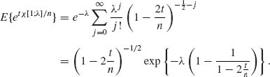
5.2.2 Let X1, …, Xn be i.i.d. random variables having an exponential distribution, E(λ), 0 < λ < ∞.
where T = ![]() and a+ = max (a, 0).
and a+ = max (a, 0).
where P(j; λ) is the c.d.f. of P(λ) and H(k| x) = ![]() . [H(k| x) can be determined recursively by the relation
. [H(k| x) can be determined recursively by the relation
![]()
and H(1|x) is the exponential integral (Abramowitz and Stegun, 1968).
5.2.3 Let X1, …, Xn be i.i.d. random variables having a two–parameter exponential distribution, X1 ∼ μ + G(λ, 1). Derive the UMVU estimators of μ and λ and their covariance matrix.
5.2.4 Let X1, …, Xn be i.i.d. N(μ, 1) random variables.
5.2.5 Consider Example 5.4. Find the variances of the UMVU estimators of p(0; λ) and of p(1; λ). [Hint: Use the formula of the p.g.f. of a P(nλ).]
5.2.6 Let X1, …, Xn be i.i.d. random variables having a NB(![]() , ν) distribution; 0 <
, ν) distribution; 0 < ![]() < ∞ (ν known). Prove that the UMVU estimator of
< ∞ (ν known). Prove that the UMVU estimator of ![]() is
is
![]()
5.2.7 Let X1, …, Xn be i.i.d. random variables having a binomial distribution B(N, θ), 0 < θ < 1.
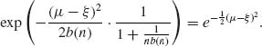
5.2.8 Let X1, …, Xn be i.i.d. N(μ, 1) random variables. Find a constant b(n) so that
![]()
is a UMVU estimator of the p.d.f. of X at ξ, i.e., ![]() . [Hint: Apply the m.g.f. of (
. [Hint: Apply the m.g.f. of (![]() – ξ)2.]
– ξ)2.]
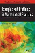
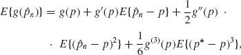
5.2.9 Let J1, …, Jn be i.i.d. random variables having a binomial distribution B(1, e-Δ/θ), 0 < θ < 1 (Δ known). Let ![]() n =
n =  . Consider the estimator of θ
![]()
Determine the bias of ![]() n as a power–series in 1/n.
n as a power–series in 1/n.
5.2.10 Let X1, …, Xn be i.i.d. random variables having a binomial distribution B(N, θ), 0 < θ < 1. What is the Cramér – Rao lower bound to the variance of the UMVU estimator of ω = θ (1-θ)?
5.2.11 Let X1, …, Xn be i.i.d. random variables having a negative–binomial distribution NB(![]() , ν). What is the Cramér – Rao lower bound to the variance of the UMVU estimator of
, ν). What is the Cramér – Rao lower bound to the variance of the UMVU estimator of ![]() ? [See Problem 6.]
? [See Problem 6.]
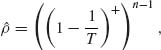
5.2.12 Derive the Cramér – Rao lower bound to the variance of the UMVU estimator of δ = e– λ in Problem 2.
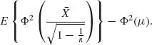
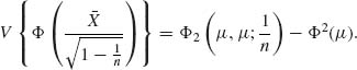
5.2.13 Derive the Cramér – Rao lower bound to the variance of the UMVU estimator of Φ(μ) in Problem 4.
5.2.14 Derive the BLBs of the second and third order for the UMVU estimator of Φ(μ) is Problem 4.
5.2.15 Let X1, …, Xn be i.i.d. random variables having a common N(μ, σ2) distribution, -∞ < μ < ∞, 0 < σ2 < ∞.
5.2.16 Let X1, …, Xn be i.i.d. random variables having a common N(μ, σ2) distribution, -∞ < μ < ∞, 0 < σ < ∞. Determine the Cramér – Rao lower bound for the variance of the UMVU estimator of ω = μ + zγ σ, where zγ = Φ−1(γ), 0 < γ < 1.
5.2.17 Let X1, …, Xn be i.i.d. random variables having a G(λ, ν) distribution, 0 < λ < ∞, ν ≥ 3 fixed.
5.2.18 Consider Example 5.8. Show that the Cramér – Rao lower bound for the variance of the MVU estimator of cov(X, Y) = ρ σ2 is ![]() .
.
5.2.19 Let X1, …, Xn be i.i.d. random variables from N(μ1, ![]() ) and Y1, …, Yn i.i.d. from N(μ2,
) and Y1, …, Yn i.i.d. from N(μ2, ![]() ). The random vectors X and Y are independent and n ≥ 3. Let δ =
). The random vectors X and Y are independent and n ≥ 3. Let δ = ![]() .
.
5.2.20 Let X1, …, Xn be i.i.d. random variables having a rectangular distribution R(0, θ), 0 < θ < ∞. Derive the Chapman – Robbins inequality for the UMVU of θ.
5.2.21 Let X1, …, Xn be i.i.d. random variables having a Laplace distribution L(μ, σ), -∞ < μ < ∞, 0 < σ < ∞. Derive the Chapman – Robbins inequality for the variances of unbiased estimators of μ.
Section 5.3
5.3.1 Show that if ![]() (X) is a biased estimator of θ, having a differentiable bias function B(θ), then the efficiency of
(X) is a biased estimator of θ, having a differentiable bias function B(θ), then the efficiency of ![]() (X), when the regularity conditions hold, is
(X), when the regularity conditions hold, is
![]()
5.3.2 Let X1, …, Xn be i.i.d. random variables having a negative exponential distribution G(λ, 1), 0 < λ < ∞.
5.3.3 Consider Example 5.8.
 .
.Section 5.4
5.4.1 Let X1, …, Xn be equicorrelated random variables having a common unknown mean μ. The variance of each variable is σ2 and the correlation between any two variables is ρ = 0.7.
5.4.2 Let X1, X2, X3 be i.i.d. random variables from a rectangular distribution R(μ – σ, μ + σ), -∞ < μ < ∞, 0 < σ < ∞. What is the best linear combination of the order statistics X(i), i = 1, 2, 3, for estimating μ, and what is its variance?
5.4.3 Suppose that X1, …, Xn are i.i.d. from a Laplace distribution with p.d.f. f(x;μ, σ) = ![]() , where
, where ![]() (z) =
(z) = ![]() . What is the best linear unbiased combination of X(1), Me, and X(n) for estimating μ, when n = 5?
. What is the best linear unbiased combination of X(1), Me, and X(n) for estimating μ, when n = 5?
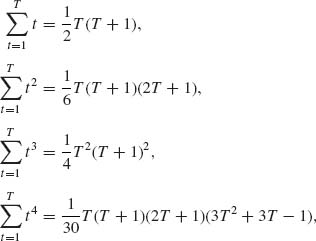
5.4.4 Let ![]() k(T) =
k(T) = ![]() .
.
![]()

[Hint: To prove (i), show that both sides are ![]() (Anderson, 1971, p. 83).]
(Anderson, 1971, p. 83).]
5.4.5 Let Xt = f(t) + et, where t = 1, …, T, where
![]()
et are uncorrelated random variables, with E{et} = 0, V{et} = σ2 for all t = 1, …, T.
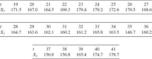
5.4.6 The annual consumption of meat per capita in the United States during the years 1919 – 1941 (in pounds) is (Anderson, 1971, p. 44)
5.4.7 Let (x1i, Y1i), i = 1, …, n1, and (x2i, Y2i), i = 1, …, n2, be two independent sets of regression points. It is assumed that
![]()
where xji are constants and eji are i.i.d. N(0, σ2). Let
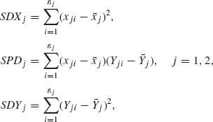
where ![]() j and
j and ![]() j are the respective sample means.
j are the respective sample means.
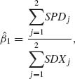
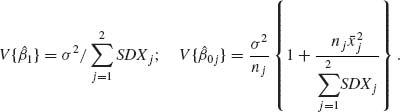
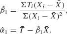
and that the LSEs of β0j (j = 1, 2) are
![]()
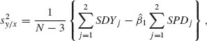
where N = n1 + n2.
Section 5.5
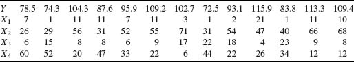
5.5.1 Consider the following raw data (Draper and Smith, 1966, p. 178).
Section 5.6
5.6.1 Let X1, …, Xn be i.i.d. random variables having a binomial distribution B(1, θ), 0 < θ < 1. Find the MLE of
5.6.2 Let X1, …, Xn be i.i.d. P(λ), 0 < λ < ∞. What is the MLE of p(j;λ) = e–λ · λj/j!, j = 0, 1, …?
5.6.3 Let X1, …, Xn be i.i.d. N(μ, σ2), -∞ < μ < ∞, 0 < σ < ∞. Determine the MLEs of
5.6.4 Using the delta method (see Section 1.13.4), determine the large sample approximation to the expectations and variances of the MLEs of Problems 1, 2, and 3.
5.6.5 Consider the normal regression model
![]()
where x1, …, xn are constants such that ![]() , and e1, …, en are i.i.d. N(0, σ2).
, and e1, …, en are i.i.d. N(0, σ2).
5.6.6 Let (xi, Ti), i = 1, …, n be specified in the following manner. x1, …, xn are constants such that ![]() are independent random variables and Ti ∼
are independent random variables and Ti ∼ ![]() , i = 1 = 1, …, n.
, i = 1 = 1, …, n.
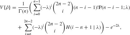
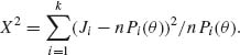
5.6.7 Consider the MLE of the parameters of the normal, logistic, and extreme–value tolerance distributions (Section 5.6.6). Let x1 < … < xk be controlled experimental levels, n1, …, nk the sample sizes and J1, …, Jk the number of response cases from those samples. Let pi = (Ji + 1/2)/(ni + 1). The following transformations:
![]()
is minimal; or

is maximal. Determine W2 and D2 to each one of the above models, according to the data in (iii), and infer which one of the three models better fits the data.
5.6.8 Consider a trinomial according to which (J1, J2) has the trinomial distribution M(n, P(θ)), where
![]()
This is the Hardy – Weinberg model.
![]()
5.6.9 A minimum chi–squared estimator (MCE) of θ in a multinomial model M(n, P(θ)) is an estimator ![]() n minimizing
n minimizing
For the model of Problem 8, show that the MCE of θ is the real root of the equation
![]()
Section 5.7
5.7.1 Let X1, …, Xn be i.i.d. random variables having a common rectangular distribution R(0, θ), 0 < θ < ∞.
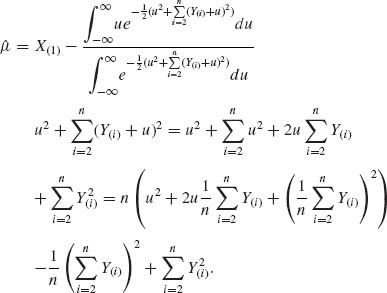
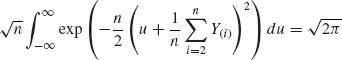
5.7.2 Let X1, …, Xn be i.i.d. random variables having a common location–parameter Cauchy distribution, i.e., f(x;μ) = ![]() , -∞ < x < ∞; -∞ < μ < ∞. Show that the Pitman estimator of μ is
, -∞ < x < ∞; -∞ < μ < ∞. Show that the Pitman estimator of μ is
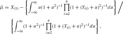
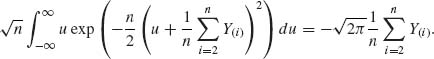
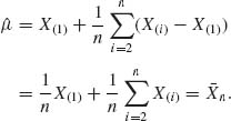
where Y(i) = X(i) – X(1), i = 2, …, n. Or, by making the transformation ω = (1 + u2)−1 one obtains the expression
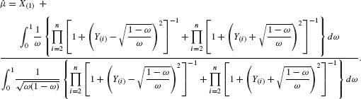
This estimator can be evaluated by numerical integration.
5.7.3 Let X1, …, Xn be i.i.d. random variables having a N(μ, σ2) distribution. Determine the Pitman estimators of μ and σ, respectively.
5.7.4 Let X1, …, Xn be i.i.d. random variables having a location and scale parameter p.d.f. f(x;μ, σ) = ![]() , where -∞ < μ < ∞, 0 < σ < ∞ and
, where -∞ < μ < ∞, 0 < σ < ∞ and ![]() (z) is of the form
(z) is of the form
Determine the Pitman estimators of μ and σ for (i) and (ii).
Section 5.8
5.8.1 Let X1, …, Xn be i.i.d. random variables. What are the MEEs of the parameters of
 known,
5.8.2 It is a common practice to express the degree and skewness and kurtosis (peakness) of a p.d.f. by the coefficients
![]()
and
![]()
Provide MEEs of ![]() and β2 based on samples of n i.i.d. random variables X1, …, Xn.
and β2 based on samples of n i.i.d. random variables X1, …, Xn.
5.8.3 Let X1, …, Xn be i.i.d. random variables having a common distribution which is a mixture α G(λ, ν1) + (1 – α) G(λ, ν2), 0 < α < 1, 0 < λ, ν1, ν2 < ∞. Construct the MEEs of α, λ, ν1, and ν2.
5.8.4 Let X1, …, Xn be i.i.d. random variables having a common truncated normal distribution with p.d.f.
![]()
where n(x| μ, σ2) = 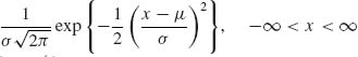 . Determine the MEEs of (μ, σ, ξ).
Section 5.9
5.9.1 Consider the fixed–effects two–way ANOVA (Section 4.6.2). Accordingly, Xijk, i = 1, …, r1; j = 1, … r2, k = 1, …, n, are independent normal random variables, N(μ ij, σ2), where
![]()
Construct PTEs of the interaction parameters ![]() and the main–effects
and the main–effects ![]()
![]() (i = 1, …, r1; j = 1, …, r2). [The estimation is preceded by a test of significance. If the test indicates nonsignificant effects, the estimates are zero; otherwise they are given by the value of the contrasts.]
(i = 1, …, r1; j = 1, …, r2). [The estimation is preceded by a test of significance. If the test indicates nonsignificant effects, the estimates are zero; otherwise they are given by the value of the contrasts.]
5.9.2 Consider the linear model Y = Aβ + e, where Y is an N× 1 vector, A is an N × p matrix (p < N) and β a p× 1 vector. Suppose that rank (A) = p. Let β′ = (β}(1), β′(2)), where β(1) is a k× 1 vector, 1 ≤ k < p. Construct the LSE PTE of β (1). What is the expectation and the covariance of this estimator?
5.9.3 Let ![]() be the sample variance of n1 i.i.d. random variables having a N(μ1,
be the sample variance of n1 i.i.d. random variables having a N(μ1, ![]() ) distribution and
) distribution and ![]() the sample variance of n2 i.i.d. random variables having a N(μ2,
the sample variance of n2 i.i.d. random variables having a N(μ2, ![]() ) distribution. Furthermore,
) distribution. Furthermore, ![]() and
and ![]() are independent. Construct PTEs of
are independent. Construct PTEs of ![]() and
and ![]() . What are the expectations and variances of these estimators? For which level of significance, α, these PTEs have a smaller MSE than
. What are the expectations and variances of these estimators? For which level of significance, α, these PTEs have a smaller MSE than ![]() and
and ![]() separately.
separately.
Section 5.10
5.10.1 What is the asymptotic distribution of the sample median Me when the i.i.d. random variables have a distribution which is the mixture
![]()
L(μ, σ) designates the Laplace distribution with location parameter μ and scale parameter σ.
5.10.2 Suppose that X(1) ≤ … ≤ X(9) is the order statistic of a random sample of size n = 9 from a rectangular distribution R(μ – σ, μ + σ). What is the expectation and variance of
5.10.3 Simulate N = 1000 random samples of size n = 20 from the distribution of X∼ 10 + 5t[10]. Estimate in each sample the location parameter μ = 10 by ![]() , Me, GL,
, Me, GL, ![]() .10 and compare the means and MSEs of these estimators over the 1000 samples.
.10 and compare the means and MSEs of these estimators over the 1000 samples.
PART IV: SOLUTIONS OF SELECTED PROBLEMS
5.2.1
![]()
where U(1) < … < U(n) are the order statistics of n i.i.d. R(0, 1) random variables. The p.d.f. of U(i), i = 1, …, n is
![]()
Thus, Ui ∼ Beta(i, n – i + 1). Accordingly
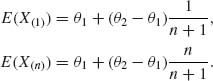
Solving the equations
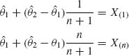
for ![]() 1 and
1 and ![]() 2, we get UMVU estimators
2, we get UMVU estimators
![]()
and
![]()
![]()
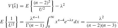
5.2.3 The m.s.s. is nX(1) and U = ![]() ;
;
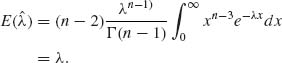
Thus ![]() is UMVU of λ, provided n> 2. X(1) ∼ μ + G(nλ, 1). Thus, E
is UMVU of λ, provided n> 2. X(1) ∼ μ + G(nλ, 1). Thus, E![]() , since E{U} =
, since E{U} = ![]() . Thus,
. Thus, ![]() = X(1) –
= X(1) – ![]() is a UMVU.
is a UMVU.
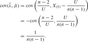
Thus,
![]()
provided n> 3. Since X(1) and U are independent,
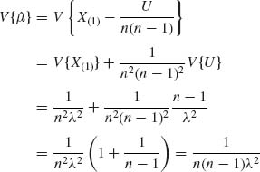
for n> 1.
5.2.4
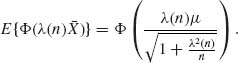
Set 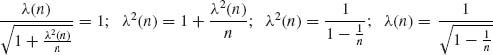 . The UMVU estimator of Φ(μ) is Φ
  .
.
is
If Y ∼ N(η, τ2) then
![]()
In our case,
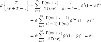
5.2.6 X1, …, Xn ∼ i.i.d. NB(![]() , ν), 0 <
, ν), 0 < ![]() < ∞ ν is known. The m.s.s. is T =
< ∞ ν is known. The m.s.s. is T = ![]() .
.
5.2.8 ![]() . Hence,
. Hence, ![]() , where
, where ![]() . Therefore,
. Therefore,
Set t = ![]() we get
we get
Thus, ![]() or
or ![]() .
.
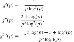
5.2.9 The probability of success is p = e-Δ/θ. Accordingly, θ = -Δ/log (p). Let ![]() . Thus,
. Thus, ![]() . The estimator of θ is
. The estimator of θ is ![]() n = -Δ/log (
n = -Δ/log (![]() n). The bias of
n). The bias of ![]() n is B(
n is B(![]() n) = -Δ
n) = -Δ ![]() . Let
. Let ![]() . Taylor expansion around p yields
. Taylor expansion around p yields
where |p -p| < |![]() n – p|. Moreover,
n – p|. Moreover,
Furthermore,
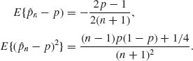
Hence,
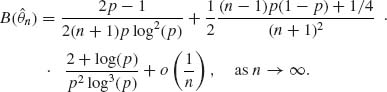
5.2.17 X1, …, Xn ∼ G(λ, ν), ν ≥ 3 fixed.
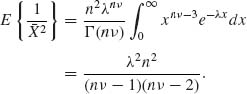
The UMVU of λ2 is ![]() .
.
![]()
![]()
![]()
The second order BLB is
![]()
and third and fourth order BLB do not exist.
5.3.3 This is continuation of Example 5.8. We have a sample of size n of vectors (X, Y), where ![]() . We have seen that
. We have seen that ![]() . We derive now the variance of
. We derive now the variance of ![]() 2 = (QX + QY)/2n, where QX =
2 = (QX + QY)/2n, where QX = ![]() and QY =
and QY = ![]() . Note that QY| QX ∼ σ2(1 – ρ2)χ2
. Note that QY| QX ∼ σ2(1 – ρ2)χ2![]() . Hence,
. Hence,
![]()
and
![]()
It follows that
![]()
Finally, since (QX + QY, PXY) is a complete sufficient statistic, and since ![]() is invariant with respect to translations and change of scale, Basu’s Theorem implies that
is invariant with respect to translations and change of scale, Basu’s Theorem implies that ![]() 2 and
2 and ![]() are independent. Hence, the variance – covariance matrix of (
are independent. Hence, the variance – covariance matrix of (![]() 2,
2, ![]() ) is
) is
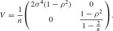
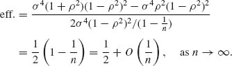
Thus, the efficiency of (![]() 2,
2, ![]() ), according to (5.3.13), is
), according to (5.3.13), is
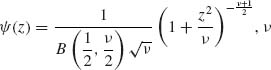
5.4.3 X1, …, X5 are i.i.d. having a Laplace distribution with p.d.f. ![]() , where -∞ < μ < ∞, 0 < σ < ∞, and
, where -∞ < μ < ∞, 0 < σ < ∞, and ![]() (x) =
(x) = ![]() , -∞ < x < ∞. The standard c.d.f. (μ = 0, σ = 1) is
, -∞ < x < ∞. The standard c.d.f. (μ = 0, σ = 1) is
![]()
Let X(1) < X(2) < X(3) < X(4) < X(5) be the order statistic. Note that Me = X(3). Also X(i) = μ + σ U(i), i = 1, …, 5, where U(i) are the order statistic from a standard distribution.
The densities of U(1), U(3), U(5) are
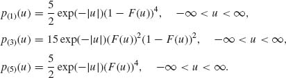
Since ![]() (u) is symmetric around u = 0, F(-u) = 1-F(u). Thus, p(3)(u) is symmetric around u = 0, and U(1) ∼ -U(5). It follows that α1 = E{U(1)} = – α5 and α3 = 0. Moreover,
(u) is symmetric around u = 0, F(-u) = 1-F(u). Thus, p(3)(u) is symmetric around u = 0, and U(1) ∼ -U(5). It follows that α1 = E{U(1)} = – α5 and α3 = 0. Moreover,

Accordingly, α′ = (-1.58854, 0, 1.58854), V{U(1)} = V{U(5)} = 1.470256, V{U(3)} = 0.35118.
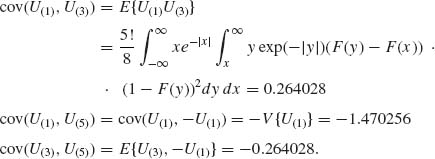
Thus,
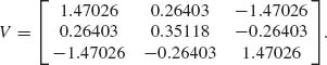
Let
The matrix V is singular, since U(5) = -U(1). We take the generalized inverse
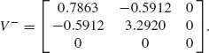
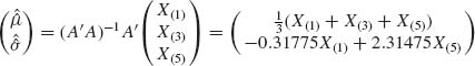
We then compute
![]()
According to this, the estimator of μ is ![]() = X(3), and that of σ is
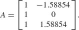
= X(3), and that of σ is ![]() = 0.63X(3)-0.63X(1). These estimators are not BLUE. Take the ordinary LSE given by
= 0.63X(3)-0.63X(1). These estimators are not BLUE. Take the ordinary LSE given by
then the variance covariance matrix of these estimators is
![]()
Thus, V{![]() } = 0.0391 < V{
} = 0.0391 < V{![]() } = 0.3512, and V{
} = 0.3512, and V{![]() } = 0.5827 > V{
} = 0.5827 > V{![]() } = 0.5125. Due to the fact that V is singular,
} = 0.5125. Due to the fact that V is singular, ![]() is a better estimator than
is a better estimator than ![]() .
.
5.6.6 (xi, Ti), i = 1, …, n. Ti ∼ (α + β xi)G(1, 1), i = 1, …, n.
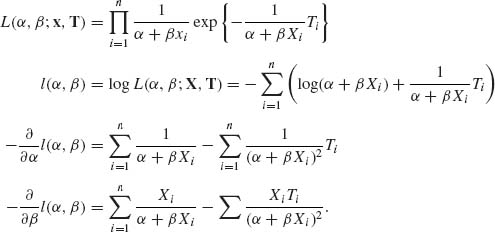
The MLEs of α and β are the roots of the equations:
(I)![]()
(II)![]() ,
,
The Newton – Raphson method for approximating numerically (α, β) is
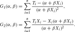
The matrix
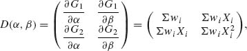
where wi = ![]() .
.
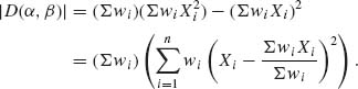
We assume that |D(α, β)| > 0 in each iteration. Starting with (α1, β1), we get the following after the lth iteration:
![]()
The LSE initial solution is
5.6.9 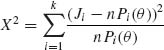 . For the Hardy – Weinberg model,
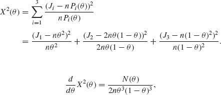
where
![]()
Note that J3 = n – J1 – J2. Thus, the MCE of θ is the root of N(θ) ≡ 0.
5.7.1 X1, …, Xn are i.i.d. R(θ, θ), 0 < θ < ∞.
![]()
Consider the following invariant loss function:
![]()
There is only one orbit of ![]() in Θ. Thus, find
in Θ. Thus, find ![]() to minimize
to minimize
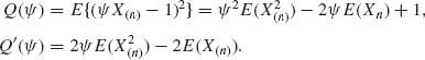
Thus, ![]() computed at θ = 1. Note that under θ = 1, X(n) ∼ Beta(n, 1) E(Xn =
computed at θ = 1. Note that under θ = 1, X(n) ∼ Beta(n, 1) E(Xn = ![]() .
.
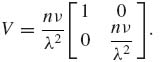
5.7.3
Moreover,
and
The other terms are cancelled. Thus,
This is the best equivariant estimator for the squared error loss.
 . An equivariant estimator of σ, for the translation–scale group, is
![]()
![]() . By Basu’s Theorem, S is independent of u. We find
. By Basu’s Theorem, S is independent of u. We find ![]() (u) by minimizing E{(S
(u) by minimizing E{(S![]() -1)2} under σ = 1. E(S2|
-1)2} under σ = 1. E(S2| ![]() ) = E1{S2} = 1 and E1{S|
) = E1{S2} = 1 and E1{S| ![]() } = E1{S}. Here,
} = E1{S}. Here, ![]() 0 = E1{S}/E1{S2}.
0 = E1{S}/E1{S2}.