
PART II: EXAMPLES
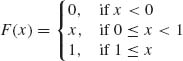
Example 1.1 We illustrate here two algebras.
The sample space is finite
![]()
Let E1 = {1, 2}, E2 = {9, 10}. The algebra generated by E1 and E2, ![]() 1, contains the events
1, contains the events
![]()
The algebra generated by the partition ![]() = {E1, E2, E3, E4}, where E1 = {1, 2}, E2 = {9, 10}, E3 = {3, 4, 5}, E4 = {6, 7, 8} contains the 24 = 16 events
= {E1, E2, E3, E4}, where E1 = {1, 2}, E2 = {9, 10}, E3 = {3, 4, 5}, E4 = {6, 7, 8} contains the 24 = 16 events
![]()
Notice that the complement of each set in ![]() 2 is in
2 is in ![]() 2.
2. ![]() 1
1 ![]()
![]() 2. Also,
2. Also, ![]() 2
2 ![]()
![]() (
(![]() ).
). ![]()
Example 1.2 In this example we consider a random walk on the integers. Consider an experiment in which a particle is initially at the origin, 0. In the first trial the particle moves to +1 or to −1. In the second trial it moves either one integer to the right or one integer to the left. The experiment consists of 2n such trials (1 ≤ n < ∞). The sample space ![]() is finite and there are 22n points in
is finite and there are 22n points in ![]() , i.e.,
, i.e., ![]() = {(i1, …, i2n): ij = ± 1, j = 1, …, 2n}. Let Ej =
= {(i1, …, i2n): ij = ± 1, j = 1, …, 2n}. Let Ej = 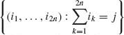 , j = 0, ± 2, ±, ···, ± 2n. Ej is the event that, at the end of the experiment, the particle is at the integer j. Obviously, −2n ≤ j ≤ 2n. It is simple to show that j must be an even integer j = ± 2k, k = 0, 1, …, n. Thus,
 ![]() = {E2k, k = 0, ± 1, …, ± n} is a partition of
= {E2k, k = 0, ± 1, …, ± n} is a partition of ![]() . The event E2k consists of all elementary events in which there are (n+k) +1s and (n−k) −1s. Thus, E2k is the union of
. The event E2k consists of all elementary events in which there are (n+k) +1s and (n−k) −1s. Thus, E2k is the union of ![]() points of
points of ![]() , k = 0, ± 1, …, ± n.
, k = 0, ± 1, …, ± n.
The algebra generated by ![]() ,
, ![]() (
(![]() ), consists of
), consists of ![]() and 22n+1−1 unions of the elements of
and 22n+1−1 unions of the elements of ![]() .
. ![]()
Example 1.3 Let ![]() be the real line, i.e.,
be the real line, i.e., ![]() = {x: −∞ < x < ∞ }. We construct an algebra
= {x: −∞ < x < ∞ }. We construct an algebra ![]() generated by half–closed intervals: Ex = (−∞, x], −∞ < x < ∞. Notice that, for x < y, Ex
generated by half–closed intervals: Ex = (−∞, x], −∞ < x < ∞. Notice that, for x < y, Ex![]() Ey = (−∞, y]. The complement of Ex is
Ey = (−∞, y]. The complement of Ex is ![]() x = (x, ∞). We will adopt the convention that (x, ∞) ≡ (x, ∞].
x = (x, ∞). We will adopt the convention that (x, ∞) ≡ (x, ∞].
Consider the sequence of intervals ![]() , n ≥ 1. All En
, n ≥ 1. All En ![]()
![]() . However,
. However, ![]() En = (−∞, 1). Thus
En = (−∞, 1). Thus ![]() En does not belong to
En does not belong to ![]() .
. ![]() is not a σ–field. In order to make
is not a σ–field. In order to make ![]() into a σ–field we have to add to it all limit sets of sequences of events in
into a σ–field we have to add to it all limit sets of sequences of events in ![]() .
. ![]()
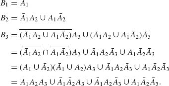
Example 1.4. We illustrate here three events that are only pairwise independent.
Let ![]() = {1, 2, 3, 4}, with P(w) =
= {1, 2, 3, 4}, with P(w) = ![]() , for all w
, for all w ![]()
![]() . Define the three events
. Define the three events
![]()
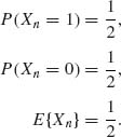
P{Ai} = ![]() , i = 1, 2, 3.
, i = 1, 2, 3.
Thus
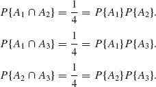
Thus, A1, A2, A3 are pairwise independent. On the other hand,
![]()
and
![]()
Thus, the triplet (A1, A2, A3) is not independent. ![]()
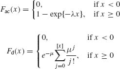
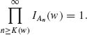
Example 1.5 An infinite sequence of trials, in which each trial results in either “success” S or “failure” F is called Bernoulli trials if all trials are independent and the probability of success in each trial is the same. More specifically, consider the sample space of countable sequences of Ss and Fs, i.e.,
![]()
Let
![]()
We assume that {E1, E2, …, En} are mutually independent for all n ≥ 2 and P{Ej} = p for all j = 1, 2, …, 0 < p < 1.
The points of ![]() represent an infinite sequence of Bernoulli trials. Consider the events
represent an infinite sequence of Bernoulli trials. Consider the events
![]()
j = 1, 2, …. {Aj} are not independent.
Let Bj = {A3j+1}, j ≥ 0. The sequence {Bj, j≥ 1} consists of mutually independent events. Moreover, P(Bj) = p2(1−p) for all j = 1, 2, …. Thus, ![]() p(Bj) = ∞ and the Borel–Cantelli Lemma implies that P{Bn, i.o.} = 1. That is, the pattern SFS will occur infinitely many times in a sequence of Bernoulli trials, with probability one.
p(Bj) = ∞ and the Borel–Cantelli Lemma implies that P{Bn, i.o.} = 1. That is, the pattern SFS will occur infinitely many times in a sequence of Bernoulli trials, with probability one. ![]()
Example 1.6. Let ![]() be the sample space of N = 2n binary sequences of size n, n <∞, i.e.,
be the sample space of N = 2n binary sequences of size n, n <∞, i.e.,
![]()
We assign the points w = (i1, …, in) of ![]() , equal probabilities, i.e., P{(i1, …, in)} = 2−n. Consider the partition
, equal probabilities, i.e., P{(i1, …, in)} = 2−n. Consider the partition ![]() = {B0, B1, …, Bn} to k = n+1 disjoint events, such that
= {B0, B1, …, Bn} to k = n+1 disjoint events, such that
![]()
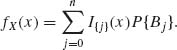
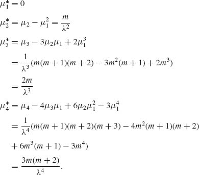
Bj is the set of all points having exactly j ones and (n−j) zeros. We define the discrete random variable corresponding to ![]() as
as
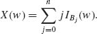
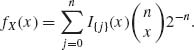
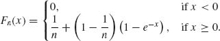
The jump points of X(w) are {0, 1, …, n}. The probability distribution function of X(w) is
It is easy to verify that
![]()
where
![]()
Thus,
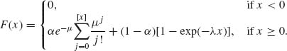
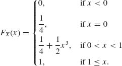
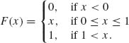
The distribution function (c.d.f.) is given by
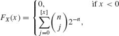
where [x] is the maximal integer value smaller or equal to x. The distribution function illustrated here is called a binomial distribution (see Section 2.2.1). ![]()
Example 1.7. Consider the random variable of Example 1.6. In that example X(w) ![]() {0, 1, …, n} and fX(j) =
{0, 1, …, n} and fX(j) = ![]() 2−n, j = 0, …, n. Accordingly,
2−n, j = 0, …, n. Accordingly,
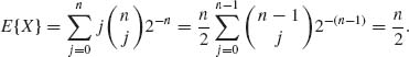
![]()
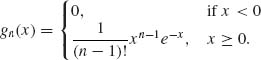
Example 1.8. Let (![]() ,
, ![]() , P) be a probability space where
, P) be a probability space where ![]() ={0, 1, 2, … }.
={0, 1, 2, … }. ![]() is the σ–field of all subsets of
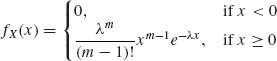
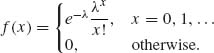
is the σ–field of all subsets of ![]() . Consider X(w) = w, with probability function
. Consider X(w) = w, with probability function
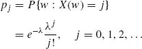
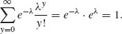
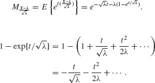
for some λ, 0 < λ < ∞. 0 < pj < ∞ for all j, and since 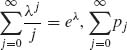 = 1.
= 1.
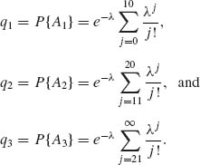
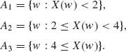
Consider the partition ![]() = {A1, A2, A3} where A1 = {w: 0 ≤ w ≤ 10}, A2 = {w: 10 < w ≤ 20} and A3 = {w: w≥ 21}. The probabilities of these sets are
= {A1, A2, A3} where A1 = {w: 0 ≤ w ≤ 10}, A2 = {w: 10 < w ≤ 20} and A3 = {w: w≥ 21}. The probabilities of these sets are
The conditional distributions of X given Ai i = 1, 2, 3 are
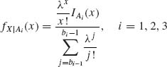
where b0 = 0, b1 = 11, b2 = 21, b3 =∞.
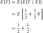
The conditional expectations are
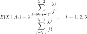
where a + = max (a, 0). E{X| ![]() } is a random variable, which obtains the values E{X| A1} with probability q1, E{X|A2} with probability q2, and E{X|A3} with probability q3.
} is a random variable, which obtains the values E{X| A1} with probability q1, E{X|A2} with probability q2, and E{X|A3} with probability q3. ![]()
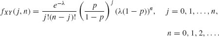
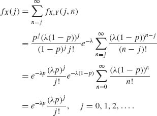
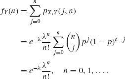
Example 1.9. Consider two discrete random variables X, Y on (![]() ,
, ![]() , P) such that the jump points of X and Y are the nonnegative integers {0, 1, 2, … }. The joint probability function of (X, Y) is
, P) such that the jump points of X and Y are the nonnegative integers {0, 1, 2, … }. The joint probability function of (X, Y) is
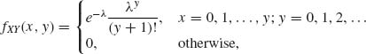
where λ, 0 < λ <∞, is a specified parameter.
First, we have to check that
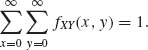
Indeed,
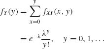
and
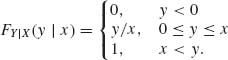
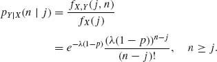
The conditional p.d.f. of X given {Y = y}, y = 0, 1, … is
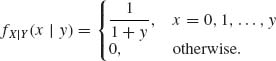
Hence,
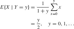
and, as a random variable,
![]()
Finally,
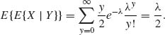
![]()
Example 1.10. In this example we show an absolutely continuous distribution for which E{X} does not exist.
Let F(x) = ![]() +
+ ![]() tan−1(x). This is called the Cauchy distribution. The density function (p.d.f.) is
tan−1(x). This is called the Cauchy distribution. The density function (p.d.f.) is
![]()
It is a symmetric density around x = 0, in the sense that f(x) = f(−x) for all x. The expected value of X having this distribution does not exist. Indeed,
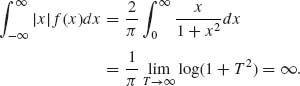
![]()
Example 1.11. We show here a mixture of discrete and absolutely continuous distributions.
Let
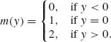
where [x] designates the maximal integer not exceeding x; λ and μ are real positive numbers. The mixed distribution is, for 0 ≤ α ≤ 1,
This distribution function can be applied with appropriate values of α, λ, and μ for modeling the length of telephone conversations. It has discontinuities at the nonnegative integers and is continuous elsewhere. ![]()
Example 1.12. Densities derived after transformations.
Let X be a random variable having an absolutely continuous distribution with p.d.f. fX.
A. If Y = X2, the number of roots are
Thus, the density of Y is
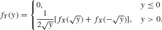
B. If Y = cos X
![]()
For every y, such that |y| < 1, let ξ (y) be the value of cos−1 (y) in the interval (0, π). Then, if f(x) is the p.d.f. of X, the p.d.f. of Y = cos X is, for |y| < 1,
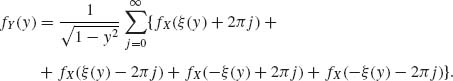
The density does not exist for |y|≥ 1. ![]()
Example 1.13. Three cases of joint p.d.f.
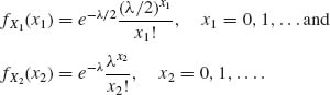
A. Both X1, X2 are discrete, with jump points on {0, 1, 2, … }. Their joint p.d.f. for 0 < λ < ∞ is,
![]()
for x1 = 0, …, x2, x2 = 0, 1, …. The marginal p.d.f. are
B. Both X1 and X2 are absolutely continuous, with joint p.d.f.
![]()
The marginal distributions of X1 and X2 are
![]()
C. X1 is discrete with jump points {0, 1, 2, … } and X2 absolutely continuous. The joint p.d.f., with respect to the σ–finite measure dN(x1)dy is, for 0 < λ <∞,
![]()
The marginal p.d.f. of X1, is
![]()
The marginal p.d.f. of X2 is

![]()
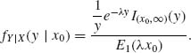
Example 1.14. Suppose that X, Y are positive random variables, having a joint p.d.f.
![]()
The marginal p.d.f. of X is
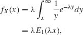
where ![]() du is called the exponential integral, which is finite for all ξ > 0. Thus, according to (1.6.62), for x0 > 0,
du is called the exponential integral, which is finite for all ξ > 0. Thus, according to (1.6.62), for x0 > 0,
Finally, for x0 > 0,
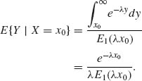
![]()
Example 1.15. In this example we show a distribution function whose m.g.f., M, exists only on an interval (−∞, t0). Let
![]()
where 0 < λ < ∞. The m.g.f. is
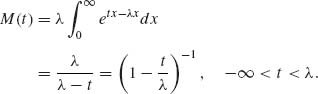
The integral in M(t) is ∞ if t ≥ λ. Thus, the domain of convergence of M is (−∞, λ). ![]()
Example 1.16. Let
![]()
i = 1, …, n. We assume also that X1, …, Xn are independent. We wish to derive the p.d.f. of Sn = ![]() Xi. The p.g.f. of Sn is, due to independence, when q = 1−p,
Xi. The p.g.f. of Sn is, due to independence, when q = 1−p,
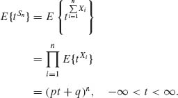
Since all Xi have the same distribution. Binomial expansion yields
![]()
Since two polynomials of degree n are equal for all t only if their coefficients are equal, we obtain
![]()
The distribution of Sn is called the binomial distribution. ![]()
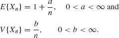
Example 1.17. In Example 1.13 Part C, the conditional p.d.f. of X2 given {X1 = x} is
![]()
This is called the uniform distribution on (0, 1+x). It is easy to find that
![]()
and
![]()
Since the p.d.f. of X is
![]()
the law of iterated expectation yields
since E{X} = λ.
The law of total variance yields
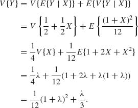
To verify these results, prove that E{X} = λ, V{X} = λ and E{X2} = λ (1 + λ). We also used the result that V{a + b X} = b2V{X}. ![]()
Example 1.18. Let X1, X2, X3 be uncorrelated random variables, having the same variance σ2, i.e.,
![]()
Consider the linear transformations
![]()
and
![]()
In matrix notation
![]()
where
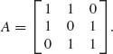
The variance–covariance matrix of Y, according to (1.8.30) is
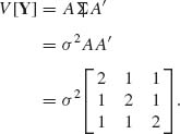
From this we obtain that correlations of Yi, Yj for i≠ j and ρij = ![]() .
. ![]()
Example 1.19. We illustrate here convergence in distribution.
A. Let X1, X2, … be random variables with distribution functions
Xn![]() X, where the distribution of X is
X, where the distribution of X is
![]()
B. Xn are random variables with
![]()
and F(x) = I{x ≥ 0}. Xn ![]() X. Notice that F(x) is discontinuous at x = 0. But, for all x≠ 0
X. Notice that F(x) is discontinuous at x = 0. But, for all x≠ 0 ![]() Fn(x) = F(x).
Fn(x) = F(x).
C. Xn are random vectors, i.e.,
![]()
The function Ix(a, b), for 0 < a, b <∞, 0 ≤ x ≤ 1, is called the incomplete beta function ratio and is given by
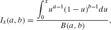
where B(a, b) = ![]() ua−1(1−u)b−1 du. In terms of these functions, the marginal distribution of X1n and X2n are
ua−1(1−u)b−1 du. In terms of these functions, the marginal distribution of X1n and X2n are
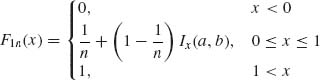
and
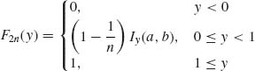
where 0 < a, b < ∞. The joint distribution of (X1n, X2n) is Fn(x, y) = F1n(x) F2n(y), n ≥ 1. The random vectors Xn![]() X, where F(x) is
X, where F(x) is
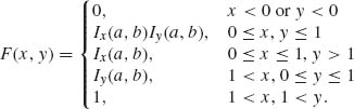
![]()
Example 1.20. Convergence in probability.
Let Xn = (X1n, X2n), where Xi, n (i = 1, 2) are independent and have a distribution
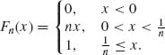
Fix an ![]() > 0 and let N(
> 0 and let N(![]() ) =
) = ![]() , then for every n > N(
, then for every n > N(![]() ),
),
![]()
Thus, Xn ![]() 0.
0. ![]()
Example 1.21. Convergence in mean square.
Let {Xn} be a sequence of random variables such that
Then, Xn ![]() 1, as n → ∞. Indeed, E{(Xn−1)2} =
1, as n → ∞. Indeed, E{(Xn−1)2} = ![]() → 0, as n→ ∞.
→ 0, as n→ ∞. ![]()
Example 1.22 Central Limit Theorem.
A. Let {Xn}, n ≥ 1 be a sequence of i.i.d. random variables, P{Xn =1} = P{Xn = −1} = ![]() . Thus, E{Xn} = 0 and V{Xn} = 1, n ≥ 1. Thus
. Thus, E{Xn} = 0 and V{Xn} = 1, n ≥ 1. Thus ![]()
![]() n =
n = ![]()
![]() Xi
Xi![]() N(0, 1). It is interesting to note that for these random variables, when Sn =
N(0, 1). It is interesting to note that for these random variables, when Sn = ![]() Xi,
Xi, ![]() Sn
Sn![]() N(0, 1), while
N(0, 1), while ![]()
![]() 0.
0.
B. Let {Xn} be i.i.d, having a rectangular p.d.f.
![]()
In this case, E{X1} = ![]() and V{X1} =
and V{X1} = ![]() . Thus,
. Thus,
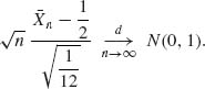
Notice that if n = 12, then if S12 = ![]() Xi, then S12−6 might have a distribution close to that of N(0, 1). Early simulation programs were based on this.
Xi, then S12−6 might have a distribution close to that of N(0, 1). Early simulation programs were based on this. ![]()
Example 1.23. Application of Lyapunov’s Theorem.
Let {Xn} be a sequence of independent random variables, with distribution functions
![]()
n ≥ 1. Thus, E{Xn} = n, V{Xn} = n2, and E{![]() } = 6n3. Thus,
} = 6n3. Thus, ![]() =
= ![]() k2 =
k2 = ![]() , n ≥ 1. In addition,
, n ≥ 1. In addition,
![]()
Thus,
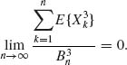
It follows from Lyapunov’s Theorem that
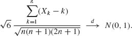
![]()
Example 1.24 Variance stabilizing transformation.
Let {Xn} be i.i.d. binary random variables, such that P{Xn = 1} = p, and P{Xn =0} = 1−p. It is easy to verify that μ = E{X1} = p and V{X1} = p(1−p). Hence, by the CLT, ![]()
![]()
![]() N(0, 1), as n → ∞. Consider the transformation
N(0, 1), as n → ∞. Consider the transformation
![]()
The derivative of g(x) is
![]()
Hence V{X1} (g(1)(p))2 = 1.
It follows that
![]()
g(2)(x) = −![]()
![]() . Hence, by the delta method,
. Hence, by the delta method,
![]()
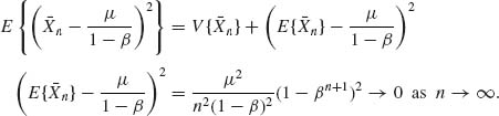
This approximation is very ineffective if p is close to zero or close to 1. If p is close to ![]() , the second term on the right–hand side is close to zero.
, the second term on the right–hand side is close to zero. ![]()
Example 1.25. A. Let X1, X2, … be i.i.d. random variables having a finite variance 0 < σ2 < ∞. Since ![]() (
(![]() n − μ)
n − μ)![]() N(0, σ2), we say that
N(0, σ2), we say that ![]() n − μ = Op
n − μ = Op ![]() as n → ∞. Thus, if cn
as n → ∞. Thus, if cn ![]() ∞ but cn = o(
∞ but cn = o(![]() ), then cn(
), then cn(![]() n − μ)
n − μ) ![]() 0. Hence
0. Hence ![]() n − μ = op(cn), as n→ ∞.
n − μ = op(cn), as n→ ∞.
B. Let X1, X2, …, Xn be i.i.d. having a common exponential distribution with p.d.f.
![]()
0 < μ < ∞. Let Yn = min [Xi, i = 1, …, n] be the first order statistic in a random sample of size n (see Section 2.10). The p.d.f. of Yn is
![]()
Thus nYn ~ X1 for all n. Accordingly, Yn = Op ![]() as n→ ∞. It is easy to see that
as n→ ∞. It is easy to see that ![]() Yn
Yn ![]() 0. Indeed, for any given
0. Indeed, for any given ![]() > 0,
> 0,
![]()
Thus, Yn = op ![]() as n→ ∞.
as n→ ∞. ![]()
PART III: PROBLEMS
Section 1.1
1.1.1 Show that A![]() B = B
B = B![]() A and AB = BA.
A and AB = BA.
1.1.2 Prove that A ![]() B = A
B = A ![]() B
B![]() , (A
, (A![]() B) − AB = A
B) − AB = A ![]()
![]()
![]() B.
B.
1.1.3 Show that if A![]() B then A
B then A![]() B = B and A
B = B and A![]() B = A.
B = A.
1.1.4 Prove DeMorgan’s laws, i.e., ![]() =
= ![]()
![]()
![]() or
or ![]() =
= ![]()
![]()
![]() .
.
1.1.5 Show that for every n ≥ 2,  .
.
1.1.6 Show that if A1 ![]() ···
··· ![]() AN then
AN then ![]() and
and ![]() An = A1.
An = A1.
1.1.7 Find ![]() .
.
1.1.8 Find ![]() .
.
1.1.9 Show that if ![]() = {A1, …, Ak} is a partition of
= {A1, …, Ak} is a partition of ![]() then, for every B, B =
then, for every B, B = ![]() .
.
1.1.10 Prove that ![]() An
An ![]()
![]() .
.
1.1.11 Prove that  and
and 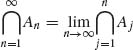 .
.
1.1.12 Show that if {An} is a sequence of pairwise disjoint sets, then  Aj =
Aj = ![]() .
.
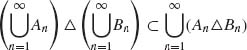
1.1.13 Prove that ![]() .
.
1.1.14 Show that if {an} is a sequence of nonnegative real numbers, then ![]() [0, an) = [0,
[0, an) = [0, ![]() an).
an).
1.1.15 Let A ![]() B = A
B = A![]()
![]() B
B![]() (symmetric difference). Let {An} be a sequence of disjoint events; define B1 = A1, Bn + 1 = Bn
(symmetric difference). Let {An} be a sequence of disjoint events; define B1 = A1, Bn + 1 = Bn ![]() An + 1, n ≥ 1. Prove that Bn =
An + 1, n ≥ 1. Prove that Bn = ![]() An.
An.
1.1.16 Verify
 .
.1.1.17 Prove that ![]() .
.
Section 1.2
1.2.1 Let ![]() be an algebra over
be an algebra over ![]() . Show that if A1, A2
. Show that if A1, A2 ![]()
![]() then A1 A2
then A1 A2 ![]()
![]() .
.
1.2.1 Let ![]() = {−, …, −2, −1, 0, 1, 2, … } be the set of all integers. A set A
= {−, …, −2, −1, 0, 1, 2, … } be the set of all integers. A set A ![]()
![]() is called symmetric if A = −A. Prove that the collection
is called symmetric if A = −A. Prove that the collection ![]() of all symmetric subsets of
of all symmetric subsets of ![]() is an algebra.
is an algebra.
1.2.3 Let ![]() = {−, …, −2, −1, 0, 1, 2…}. Let
= {−, …, −2, −1, 0, 1, 2…}. Let ![]() 1 be the algebra of symmetric subsets of
1 be the algebra of symmetric subsets of ![]() , and let
, and let ![]() 2 be the algebra generated by sets An = {−2, −1, i1, …, in}, n ≥ 1, where ij ≥ 0, j = 1, …, n.
2 be the algebra generated by sets An = {−2, −1, i1, …, in}, n ≥ 1, where ij ≥ 0, j = 1, …, n.
1.2.4 Show that if ![]() is a σ–field, An
is a σ–field, An ![]() An+1, for all n ≥ 1, then
An+1, for all n ≥ 1, then ![]()
![]() n
n ![]()
![]() .
.
Section 1.3
1.3.1 Let F(x) = P{(− ∞, x]}. Verify
(a) P{(a, b]} = F(b) − F(a).
(b) P{(a, b)} = F(b−)−F(a).
(c) P{[a, b)} = F(b−)−F(a−).
1.3.2 Prove that P{A ![]() B} = P{A} + P{B
B} = P{A} + P{B![]() }.
}.
1.3.3 A point (X, Y) is chosen in the unit square. Thus, ![]() ={(x, y): 0 ≤ x, y ≤ 1}. Let
={(x, y): 0 ≤ x, y ≤ 1}. Let ![]() be the Borel σ–field on
be the Borel σ–field on ![]() . For a Borel set B, we define
. For a Borel set B, we define
![]()
Compute the probabilities of
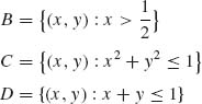
P{D![]() B}, P{D
B}, P{D![]() C}, P{C
C}, P{C ![]() B}.
B}.
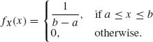
1.3.4 Let ![]() = {x: 0 ≤ x < ∞ } and
= {x: 0 ≤ x < ∞ } and ![]() the Borel σ–field on
the Borel σ–field on ![]() , generated by the sets [0, x), 0 < x < ∞. The probability function on
, generated by the sets [0, x), 0 < x < ∞. The probability function on ![]() is P{B} = λ
is P{B} = λ ![]() e−λxdx, for some 0 < λ < ∞. Compute the probabilities
e−λxdx, for some 0 < λ < ∞. Compute the probabilities
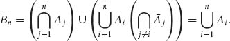
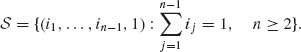
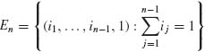
1.3.5 Consider an experiment in which independent trials are conducted sequentially. Let Ri be the result of the ith trial. P{Ri = 1} = p, P{Ri = 0} = 1−p. The trials stop when (R1, R2, …, RN) contains exactly two 1s. Notice that in this case, the number of trials N is random. Describe the sample space. Let wn be a point of ![]() , which contains exactly n trials. wn = {(i1, …, in−1, 1)}, n ≥ 2, where
, which contains exactly n trials. wn = {(i1, …, in−1, 1)}, n ≥ 2, where ![]() ij = 1. Let En = {(i1, …, in−1, 1):
ij = 1. Let En = {(i1, …, in−1, 1): ![]() ij = 1}.
ij = 1}.
1.3.6 In a parking lot there are 12 parking spaces. What is the probability that when you arrive, assuming cars fill the spaces at random, there will be four adjacent spaces vacant, while all other spaces filled?
Section 1.4
1.4.1 Show that if A and B are independent, then ![]() and
and ![]() , A and
, A and ![]() ,
, ![]() and B are independent.
and B are independent.
1.4.2 Show that if three events are mutually independent, then if we replace any event with its complement, the new collection is still mutually independent.
1.4.3 Two digits are chosen from the set ![]() = {0, 1, …, 9}, without replacement. The order of choice is immaterial. The probability function assigns every possible set of two the same probability. Let Ai(i = 0, …, 9) be the event that the chosen set contains the digit i. Show that for any i ≠ j, Ai and Aj are not independent.
= {0, 1, …, 9}, without replacement. The order of choice is immaterial. The probability function assigns every possible set of two the same probability. Let Ai(i = 0, …, 9) be the event that the chosen set contains the digit i. Show that for any i ≠ j, Ai and Aj are not independent.
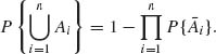
1.4.4 Let A1, …, An be mutually independent events. Show that
1.4.5 If an event A is independent of itself, then P{A} = 0 or P(A) = 1.
1.4.6 Consider the random walk model of Example 1.2.
1.4.7 Prove that
1.4.8. What is the probability that the birthdays of n = 12 randomly chosen people will fall in 12 different calendar months?
1.4.9 A stick is broken at random into three pieces. What is the probability that these pieces can form a triangle?
1.4.10 There are n = 10 particles and m = 5 cells. Particles are assigned to the cells at random.
Section 1.5
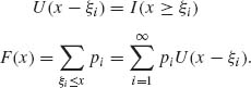
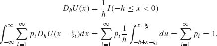
1.5.1 Let F be a discrete distribution concentrated on the jump points −∞ < ξ1 < ξ2 < ··· < ∞. Let pi = dF (ξi), i = 1, 2, …. Define the function
![]()
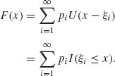
![]()
Show that
![]()
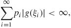 ,
,
![]()
1.5.2 Let X be a random variable having a discrete distribution, with jump points ξi = i, and pi = dF(ξi) = e−2 ![]() , i = 0, 1, 2, …. Let Y = X3. Determine the p.d.f. of Y.
, i = 0, 1, 2, …. Let Y = X3. Determine the p.d.f. of Y.
1.5.3 Let X be a discrete random variable assuming the values {1, 2, …, n} with probabilities
![]()
1.5.4 Consider a discrete random variable X, with jump points on {1, 2, … } and p.d.f.
![]()
where c is a normalizing constant.
1.5.5 Let X be a discrete random variable whose distribution has jump points at {x1, x2, …, xk}, 1 ≤ k ≤ ∞. Assume also that E{|X|} < ∞. Show that for any linear transformation Y = α + β x, β ≠ 0, −∞ < α <∞, E{Y} = α + β E{X}. (The result is trivially true for β = 0).
1.5.6 Consider two discrete random variables (X, Y) having a joint p.d.f.
1.5.7 Let X be a discrete random variable, X ![]() {0, 1, 2, … } with p.d.f.
{0, 1, 2, … } with p.d.f.
![]()
1.5.8 Consider the partition ![]() = {A1, A2, A3}, where
= {A1, A2, A3}, where
![]()
1.5.8 For a given λ, 0 < λ <∞, define the function P(j;λ) = e−![]() .
.
![]()
and where P(j;0) = I{j ≥ 0}.
1.5.9 Let X have an absolutely continuous distribution function with p.d.f.
![]()
Find E{e−X}.
Section 1.6
1.6.1 Consider the absolutely continuous distribution
of a random variable X. By considering the sequences of simple functions
![]()
and
![]()
show that
![]()
and
![]()
1.6.2 Let X be a random variable having an absolutely continuous distribution F, such that F(0) = 0 and F(1) = 1. Let f be the corresponding p.d.f.
![]()
![]()
which is the Riemann integral.
1.6.3 Let X, Y be independent identically distributed random variables and let E{X} exist. Show that
![]()
1.6.4 Let X1, …, Xn be i.i.d. random variables and let E{X1} exist. Let Sn = ![]() Xj. Then, E{X1|Sn} =
Xj. Then, E{X1|Sn} = ![]() , a.s.
, a.s.
1.6.5 Let
Find E{X} and E{X2}.
1.6.6 Let X1, …, Xn be Bernoulli random variables with P{Xi = 1} = p. If n = 100, how large should p be so that P{Sn < 100} < 0.1, when Sn = ![]() Xi?
Xi?
1.6.7 Prove that if E{|X|}<∞, then, for every A ![]()
![]() ,
,
![]()
1.6.8 Prove that if E{|X|} < ∞ and E{|Y|}<∞, then E{X + Y} = E{X} + E{Y}.
1.6.9 Let {Xn} be a sequence of i.i.d. random variables with common c.d.f.
![]()
Let Sn = ![]() Xi.
Xi.
1.6.10 Consider the distribution function F of Example 1.11, with α = .9, λ = .1, and μ = 1.
1.6.11 Consider the Cauchy distribution with p.d.f.
![]()
with μ = 10 and σ = 2.
1.6.12 Let X be a random variable having the p.d.f. f(x) = e−x, x ≥ 0. Determine the p.d.f. and the median of
1.6.13 Let X be a random variable having a p.d.f. f(x) = ![]() , −
, −![]() ≤ x ≤
≤ x ≤ ![]() . Determine the p.d.f. and the median of
. Determine the p.d.f. and the median of
1.6.14 Prove that if E{|X|} < ∞ then
![]()
1.6.15 Apply the result of the previous problem to derive the expected value of a random variable X having an exponential distribution, i.e.,
![]()
1.6.16 Prove that if F(x) is symmetric around η, i.e.,
![]()
then E{X} = η, provided E{|X|} < ∞.
Section 1.7
1.7.1 Let (X, Y) be random variables having a joint p.d.f.
![]()
1.7.2 Consider random variables {X, Y}. X is a discrete random variable with jump points {0, 1, 2, … }. The marginal p.d.f. of X is fX(x) = e−λ ![]() , x = 0, 1, …, 0 < λ < ∞. The conditional distribution of Y given {X = x}, x≥ 1, is
, x = 0, 1, …, 0 < λ < ∞. The conditional distribution of Y given {X = x}, x≥ 1, is
When {X = 0}
![]()
![]()
and prove that ![]() fY(y) dy = 1−e−λ.
fY(y) dy = 1−e−λ.
1.7.3 Show that if X, Y are independent random variables, E{|X|} < ∞ and E{|Y| < ∞ }, then E{XY} = E{X} E{Y}. More generally, if g, h are integrable, then if X, Y are independent, then
![]()
1.7.4 Show that if X, Y are independent, absolutely continuous, with p.d.f. fX and fY, respectively, then the p.d.f. of T = X + Y is
![]()
[fT is the convolution of fX and fY.]
Section 1.8
1.8.1 Prove that if E{|X|r} exists, r ≥ 1, then ![]() (a)r P{|X| ≥ a} = 0.
(a)r P{|X| ≥ a} = 0.
1.8.2 Let X1, X2 be i.i.d. random variables with E{X![]() } < ∞. Find the correlation between X1 and T = X1 + Xn.
} < ∞. Find the correlation between X1 and T = X1 + Xn.
1.8.3 Let X1, …, Xn be i.i.d. random variables; find the correlation between X1 and the sample mean ![]() n =
n = ![]()
![]() Xi.
Xi.
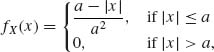
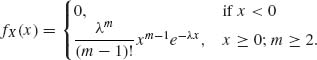
1.8.4 Let X have an absolutely continuous distribution with p.d.f.
where 0 < λ < ∞ and m is an integer, m ≥ 2.
1.8.5 Let X have an absolutely continuous distribution with p.d.f.
1.8.6 Random variables X1, X2, X3 have the covariance matrix
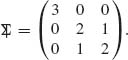
Find the variance of Y = 5x1 − 2x2 + 3x3.
1.8.7 Random variables X1, …, Xn have the covariance matrix
![]()
where J is an n × n matrix of 1s. Find the variance of ![]() n =
n = ![]()
![]() Xi.
Xi.
1.8.8 Let X have a p.d.f.
![]()
Find the characteristic function ![]() of X.
of X.
1.8.9 Let X1, …, Xn be i.i.d., having a common characteristic function ![]() . Find the characteristic function of
. Find the characteristic function of ![]() n =
n = ![]()
![]() Xj.
Xj.
1.8.10 If ![]() is a characteristic function of an absolutely continuous distribution, its p.d.f. is
is a characteristic function of an absolutely continuous distribution, its p.d.f. is
![]()
Show that the p.d.f. corresponding to
![]()
is
![]()
1.8.11 Find the m.g.f. of a random variable whose p.d.f. is
0 < a < ∞.
1.8.12 Prove that if ![]() is a characteristic function, then |
is a characteristic function, then |![]() (t)|2 is a characteristic function.
(t)|2 is a characteristic function.
1.8.13 Prove that if ![]() is a characteristic function, then
is a characteristic function, then
1.8.14 Let X be a discrete random variable with p.d.f.
Find the p.g.f. of X.
Section 1.9
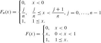
1.9.1 Let Fn, n ≥ 1, be the c.d.f. of a discrete uniform distribution on ![]() . Show that Fn(x)
. Show that Fn(x) ![]() F(x), as n→ ∞, where
F(x), as n→ ∞, where
1.9.2 Let B(j;n, p) denote the c.d.f. of the binomial distribution with p.d.f.
![]()
where 0 < p < 1. Consider the sequence of binomial distributions
![]()
What is the weak limit of Fn(x)?
1.9.3 Let X1, X2, …, Xn, … be i.i.d. random variables such that V{X1} = σ2 <∞, and μ = E{X1}. Use Chebychev’s inequality to prove that ![]() n =
n = ![]()
![]() Xi
Xi ![]() μ as n→ ∞.
μ as n→ ∞.
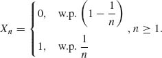
1.9.4 Let X1, X2, … be a sequence of binary random variables, such that P{Xn = 1} = ![]() , and P{Xn = 0} = 1 −
, and P{Xn = 0} = 1 − ![]() , n ≥ 1.
, n ≥ 1.
1.9.5 Let ![]() 1,
1, ![]() 2, … be independent r.v., such that E{
2, … be independent r.v., such that E{![]() n} = μ and V{
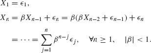
n} = μ and V{![]() n} = σ2 for all n ≥ 1. Let X1 =
n} = σ2 for all n ≥ 1. Let X1 = ![]() 1 and for n ≥ 2, let Xn = β Xn−1 +
1 and for n ≥ 2, let Xn = β Xn−1 + ![]() n, where −1 < β < 1. Show that
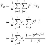
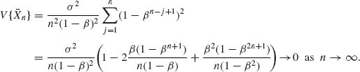
n, where −1 < β < 1. Show that ![]() n =
n = ![]()
![]() Xi
Xi![]()
![]() , as n→ ∞.
, as n→ ∞.
1.9.6 Prove that convergence in the rth mean, for some r > 0 implies convergence in the sth mean, for all 0 < s < r.
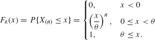
1.9.7 Let X1, X2, …, Xn, … be i.i.d. random variables having a common rectangular distribution R(0, θ), 0 < θ < ∞. Let X(n) = max {X1, …, Xn}. Let ![]() > 0. Show that
> 0. Show that ![]() Pθ {X(n) < θ −
Pθ {X(n) < θ − ![]() } < ∞. Hence, by the Borel–Cantelli Lemma, X(n)
} < ∞. Hence, by the Borel–Cantelli Lemma, X(n) ![]() θ, as n→ ∞. The R(0, θ) distribution is
θ, as n→ ∞. The R(0, θ) distribution is
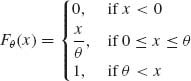
where 0 < θ < ∞.
1.9.8 Show that if Xn ![]() X and Xn
X and Xn ![]() Y, then P{w: X(w) ≠ Y(w)} = 0.
Y, then P{w: X(w) ≠ Y(w)} = 0.
1.9.9 Let Xn ![]() X, Yn
X, Yn ![]() Y, P{w: X(w) ≠ Y(w)} = 0. Then, for every
Y, P{w: X(w) ≠ Y(w)} = 0. Then, for every ![]() > 0,
> 0,
![]()
1.9.10 Show that if Xn ![]() C as n→ ∞, where C is a constant, then Xn
C as n→ ∞, where C is a constant, then Xn ![]() C.
C.
1.9.11 Let {Xn} be such that, for any p > 0, ![]() E{|Xn|p} < ∞. Show that Xn
E{|Xn|p} < ∞. Show that Xn ![]() 0 as n→ ∞.
0 as n→ ∞.
1.9.12 Let {Xn} be a sequence of i.i.d. random variables. Show that E{|X1|} < ∞ if and only if ![]() P{|X1| >
P{|X1| > ![]() · n} < ∞. Show that E|X1| < ∞ if and only if
· n} < ∞. Show that E|X1| < ∞ if and only if ![]() .
.
Section 1.10
1.10.1 Show that if Xn has a p.d.f. fn and X has a p.d.f. g(x) and if ![]() |fn(x) − g(x)|dx → 0 as n→ ∞, then
|fn(x) − g(x)|dx → 0 as n→ ∞, then ![]() |Pn{B} − P{B} | → 0 as n→ ∞, for all Borel sets B. (Ferguson, 1996, p. 12).
|Pn{B} − P{B} | → 0 as n→ ∞, for all Borel sets B. (Ferguson, 1996, p. 12).
1.10.2 Show that if a′Xn ![]() a′X as n→ ∞, for all vectors a, then Xn
a′X as n→ ∞, for all vectors a, then Xn ![]() X (Ferguson, 1996, p. 18).
X (Ferguson, 1996, p. 18).
1.10.3 Let {Xn} be a sequence of i.i.d. random variables. Let Zn = ![]() (
(![]() n − μ), n ≥ 1, where μ = E{X1} and
n − μ), n ≥ 1, where μ = E{X1} and ![]() n =
n = ![]()
![]() Xi. Let V{X1} < ∞. Show that {Zn} is tight.
Xi. Let V{X1} < ∞. Show that {Zn} is tight.
1.10.4 Let B(n, p) designate a discrete random variable, having a binomial distribution with parameter (n, p). Show that ![]() is tight.
is tight.
1.10.5 Let P(λ) designate a discrete random variable, which assumes on {0, 1, 2, … } the p.d.f. f(x) = e−λ ![]() , x = 0, 1, …, 0 < λ < ∞. Using the continuity theorem prove that B(n, pn)
, x = 0, 1, …, 0 < λ < ∞. Using the continuity theorem prove that B(n, pn)![]() P(λ) if
P(λ) if ![]() npn = λ.
npn = λ.
1.10.6 Let Xn ~ B ![]() , n ≥ 1. Compute
, n ≥ 1. Compute ![]() E{e−Xn}.
E{e−Xn}.
Section 1.11
1.11.1 (Khinchin WLLN). Use the continuity theorem to prove that if X1, X2, …, Xn, … are i.i.d. random variables, then ![]() n
n ![]() μ, where μ = E{X1}.
μ, where μ = E{X1}.
1.11.2 (Markov WLLN). Prove that if X1, X2, …, Xn, … are independent random variables and if μ k = E{Xk} exists, for all k ≥ 1, and E|Xk − μk|1+δ < ∞ for some δ > 0, all k ≥ 1, then ![]() E|Xk − μk|1+δ → 0 as n→ ∞ implies that
E|Xk − μk|1+δ → 0 as n→ ∞ implies that ![]()
![]() (Xk − μk)
(Xk − μk) ![]() 0 as n→ ∞.
0 as n→ ∞.
1.11.3 Let {Xn} be a sequence of random vectors. Prove that if ![]() n
n ![]() μ then
μ then ![]() n
n ![]() μ, where
μ, where ![]() n =
n = ![]()
![]() Xj and μ = E{X1}.
Xj and μ = E{X1}.
1.11.4 Let {Xn} be a sequence of i.i.d. random variables having a common p.d.f.
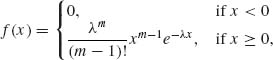
where 0 < λ <∞, m = 1, 2, …. Use Cantelli’s Theorem (Theorem 1.11.1) to prove that ![]() n
n ![]()
![]() , as n→ ∞.
, as n→ ∞.
1.11.5 Let {Xn} be a sequence of independent random variables where
![]()
and R(−n, n) is a random variable having a uniform distribution on (−n, n), i.e.,
![]()
Show that ![]() n
n ![]() 0, as n→ ∞. [Prove that condition (1.11.6) holds].
0, as n→ ∞. [Prove that condition (1.11.6) holds].
1.11.6 Let {Xn} be a sequence of i.i.d. random variables, such that |Xn| ≤ C a.s., for all n ≥ 1. Show that ![]() n
n ![]() μ as n→ ∞, where μ = E{X1}.
μ as n→ ∞, where μ = E{X1}.
1.11.7 Let {Xn} be a sequence of independent random variables, such that
![]()
and
![]()
Prove that ![]()
![]() Xi
Xi ![]() 0, as n→ ∞.
0, as n→ ∞.
Section 1.12
1.12.1 Let X ~ P(λ), i.e.,
![]()
Apply the continuity theorem to show that
![]()
1.12.2 Let {Xn} be a sequence of i.i.d. discrete random variables, and X1 ~ P(λ). Show that
![]()
What is the relation between problems 1 and 2?
1.12.3 Let {Xn} be i.i.d., binary random variables, P{Xn = 1} = P{Xn = 0} = ![]() , n ≥ 1. Show that
, n ≥ 1. Show that
where ![]() , n ≥ 1.
, n ≥ 1.
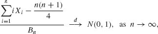
1.12.4 Consider a sequence {Xn} of independent discrete random variables, P{Xn = n} = P{Xn = −n} = ![]() , n ≥ 1. Show that this sequence satisfies the CLT, in the sense that
, n ≥ 1. Show that this sequence satisfies the CLT, in the sense that
![]()
1.12.5 Let {Xn} be a sequence of i.i.d. random variables, having a common absolutely continuous distribution with p.d.f.

Show that this sequence satisfies the CLT, i.e.,
![]()
where σ2 = V{X}.
1.12.6 (i) Show that
![]()
where G(1, n) is an absolutely continuous random variable with a p.d.f.
(ii) Show that, for large n,
![]()
Or
![]()
This is the famous Stirling approximation.
Section 1.13
1.13.1 Let Xn ~ R(−n, n), n ≥ 1. Is the sequence {Xn} uniformly integrable?
1.13.2 Let ![]() ~ N(0, 1), n ≥ 1. Show that {Zn} is uniformly integrable.
~ N(0, 1), n ≥ 1. Show that {Zn} is uniformly integrable.
1.13.3 Let {X1, X2, …, Xn, … } and {Y1, Y2, …, Yn, … } be two independent sequences of i.i.d. random variables. Assume that 0 < V{X1} = ![]() <∞, 0 < V{Y1} =
<∞, 0 < V{Y1} = ![]() < ∞. Let f(x, y) be a continuous function on R2, having continuous partial derivatives. Find the limiting distribution of
< ∞. Let f(x, y) be a continuous function on R2, having continuous partial derivatives. Find the limiting distribution of ![]() (f(
(f(![]() n,
n, ![]() n) − f(ξ, η)), where ξ = E{X1}, η = E{Y1}. In particular, find the limiting distribution of Rn =
n) − f(ξ, η)), where ξ = E{X1}, η = E{Y1}. In particular, find the limiting distribution of Rn = ![]() n/
n/ ![]() n, when η > 0.
n, when η > 0.
1.13.4 We say that X ~ E(μ), 0 < μ <∞, if its p.d.f. is
![]()
Let X1, X2, …, Xn, … be a sequence of i.i.d. random variables, X1 ~ E(μ), 0 < μ < ∞. Let ![]() n =
n = ![]()
![]() Xi.
Xi.
1.13.5 Let {Xn} be i.i.d. Bernoulli random variables, i.e., X1 ~ B(1, p), 0 < p < 1. Let ![]() n =
n = ![]()
![]() Xi and
Xi and
![]()
Use the delta method to find an approximation, for large values of n, of
Find the asymptotic distribution of ![]() .
.
1.13.6 Let X1, X2, …, Xn be i.i.d. random variables having a common continuous distribution function F(x). Let Fn(x) be the empirical distribution function. Fix a value x0 such that 0 < Fn(x0) < 1.
1.13.7 Let X1, X2, …, Xn be i.i.d. random variables having a standard Cauchy distribution. What is the asymptotic distribution of the sample median ![]() ?
?
PART IV: SOLUTIONS TO SELECTED PROBLEMS
1.1.5 For n = 2, ![]() =
= ![]() 1
1 ![]()
![]() 2. By induction on n, assume that
2. By induction on n, assume that ![]() =
= ![]()
![]() i for all k = 2, …, n. For k = n+1,
i for all k = 2, …, n. For k = n+1,
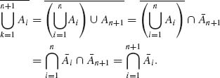
1.1.10 We have to prove that ![]() . For an elementary event w
. For an elementary event w ![]()
![]() , let
, let
![]()
Thus, if w ![]()
![]() An =
An = ![]() An, there exists an integer K(w) such that
An, there exists an integer K(w) such that
Accordingly, for all n ≥ 1, w ![]()
![]() Ak. Here w
Ak. Here w ![]()
![]()
![]() Ak =
Ak = ![]() .
.
1.1.15 Let {An} be a sequence of disjoint events. For all n ≥ 1, we define
![]()
and
By induction on n we prove that, for all n ≥ 2,
Hence Bn ![]() Bn + 1 for all n ≥ 1 and
Bn + 1 for all n ≥ 1 and ![]() Bn =
Bn = ![]() An.
An.
1.2.2. The sample space ![]() =
= ![]() , the set of all integers. A is a symmetric set in
, the set of all integers. A is a symmetric set in ![]() , if A = −A. Let
, if A = −A. Let ![]() = {collection of all symmetric sets}.
= {collection of all symmetric sets}. ![]()
![]()
![]() . If A
. If A ![]()
![]() then
then ![]()
![]()
![]() . Indeed −
. Indeed −![]() = −
= −![]() − (−A) =
− (−A) = ![]() − A =
− A = ![]() . Thus,
. Thus, ![]()
![]()
![]() . Moreover, if A, B
. Moreover, if A, B ![]()
![]() then A
then A ![]() B
B ![]()
![]() . Thus,
. Thus, ![]() is an algebra.
is an algebra.
1.2.3 ![]() =
= ![]() . Let
. Let ![]() 1 = { generated by symmetric sets }.
1 = { generated by symmetric sets }. ![]() 2 = { generated by (−2, −1, i1, …, in), n ≥ 1, ij
2 = { generated by (−2, −1, i1, …, in), n ≥ 1, ij ![]()
![]()
![]() j = 1, …, n}. Notice that if A = (−2, −1, i1, …, in) then
j = 1, …, n}. Notice that if A = (−2, −1, i1, …, in) then ![]() = {(···, −4, −3,
= {(···, −4, −3, ![]() −(i1, …, in))}
−(i1, …, in))} ![]()
![]() 2, and
2, and ![]() = A
= A![]()
![]() 1
1 ![]() A2.
A2. ![]() 2 is an algebra.
2 is an algebra. ![]() 3 =
3 = ![]() 1
1 ![]()
![]() 2. If B
2. If B ![]()
![]() 3 it must be symmetric and also B
3 it must be symmetric and also B ![]()
![]() 2. Thus, B = (−2, −1, 1, 2) or B = (···, −4, −3, 3, 4, …). Thus, B and
2. Thus, B = (−2, −1, 1, 2) or B = (···, −4, −3, 3, 4, …). Thus, B and ![]() are in
are in ![]() 3, so
3, so ![]() = (B
= (B ![]()
![]() )
) ![]()
![]() 3 and so is
3 and so is ![]() . Thus,
. Thus, ![]() is an algebra.
is an algebra.
Let ![]() 4 =
4 = ![]() 1
1 ![]()
![]() 2. Let A = {−2, −1, 3, 7} and B = {−3, 3}. Then A
2. Let A = {−2, −1, 3, 7} and B = {−3, 3}. Then A ![]() B = {−3, −2, −1, 3;7}. But A
B = {−3, −2, −1, 3;7}. But A![]() B does not belong to
B does not belong to ![]() 1 neither to
1 neither to ![]() 2. Thus A
2. Thus A![]() B
B ![]()
![]() 4.
4. ![]() 4 is not an algebra.
4 is not an algebra.
1.3.5 The sample space is
 , n = 2, 3, …. For j ≠ k, Ej
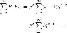
Indeed,
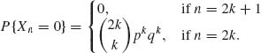
1.4.6 Let Xn denote the position of the particle after n steps.
![]()
Thus, if n = 2k+1,
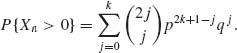
In this solution, we assumed that all steps are independent (see Section 1.7). If n = 2k the formula can be obtained in a similar manner.
Let An = {Xn = 0}. Then, ![]() P{A2k+1} = 0 and when p =
P{A2k+1} = 0 and when p = ![]() ,
,
![]()
Thus, by the Borel–Cantelli Lemma, if p = ![]() , P{An i.o.} = 1. On the other hand, if p ≠
, P{An i.o.} = 1. On the other hand, if p ≠ ![]() ,
,
![]()
Thus, if p ≠ ![]() , P{Ani.o.} = 0.
, P{Ani.o.} = 0.
1.5.1 F(x) is a discrete distribution with jump points at −∞ < ξ1 < ξ2 < ··· < ∞. pi = d(Fξi), i = 1, 2, …. U(x) = I(x ≥ 0).
![]()
U(x+h) =1 if x ≥ −h. Thus,
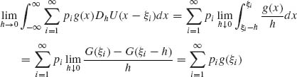
Here, G(ξi) = ![]() g(x)dx;
g(x)dx; ![]() G(ξi) = g(ξi).
G(ξi) = g(ξi).
1.5.6 The joint p.d.f. of two discrete random variables is
![]()
![]()
![]()
![]()
1.5.8
![]()
where j ≥ 1, and P(j−1;x) = e−x ![]() .
.
![]()
Fj(x) is absolutely continuous.
1.6.3 X, Y are independent and identically distributed, E|X| < ∞.
1.6.9
![]()
1.8.4
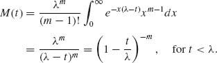
The domain of convergence is (−∞, λ).
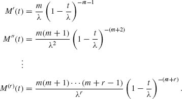
Thus, μr = M(r)(t) ![]() ≥ 1.
≥ 1.
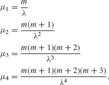
The central moments are
![]()
1.8.11 The m.g.f. is
1.9.1
All points −∞ < x < ∞ are continuity points of F(x). ![]() Fn(x) = F(x), for all x < 0 or x > 1. |Fn(x) − F(x)| ≤
Fn(x) = F(x), for all x < 0 or x > 1. |Fn(x) − F(x)| ≤ ![]() for all 0 ≤ x ≤ 1. Thus Fn(x)
for all 0 ≤ x ≤ 1. Thus Fn(x)![]() F(x), as n → ∞.
F(x), as n → ∞.
1.9.4
1.9.5 ![]() 1,
1, ![]() 2, ··· independent r.v.s, such that E(
2, ··· independent r.v.s, such that E(![]() n) = μ, and V{
n) = μ, and V{![]() n} = σ2.
n} = σ2. ![]() n ≥ 1.
n ≥ 1.
Thus, 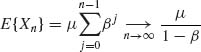 .
.
Since {![]() n} are independent,
n} are independent,
Furthermore,
Hence, ![]()
1.9.7 X1, X2, … i.i.d. distributed like R(0, θ). Xn = ![]() (Xi). Due to independence,
(Xi). Due to independence,
Accordingly, P{X(n) < θ −![]() } =
} = ![]() n, 0 <
n, 0 < ![]() < θ. Thus,
< θ. Thus, ![]() P{X(n) ≤ θ −
P{X(n) ≤ θ −![]() }<∞, and P{X(n) ≤ θ −
}<∞, and P{X(n) ≤ θ −![]() , i.o.} = 0. Hence, X(n)→ θ a.s.
, i.o.} = 0. Hence, X(n)→ θ a.s.
1.10.2 We are given that a′Xn ![]() a′X for all a. Consider the m.g.f.s, by continuity theorem Ma′Xn(t) = E{et a′Xn} → E{eta = X}, for all t in the domain of convergence. Thus E{et a)′Xn} → E{e(t a)′X} for all β = t a. Thus,
a′X for all a. Consider the m.g.f.s, by continuity theorem Ma′Xn(t) = E{et a′Xn} → E{eta = X}, for all t in the domain of convergence. Thus E{et a)′Xn} → E{e(t a)′X} for all β = t a. Thus, ![]() n
n ![]() X.
X.
1.10.6 Xn ~ B ![]()
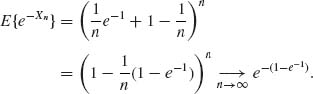
Thus, ![]() MXn (−1) = Mx(−1), where X ~ P(1).
MXn (−1) = Mx(−1), where X ~ P(1).
1.11.1
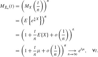
etμ is the m.g.f. of the distribution
![]()
Thus, by the continuity theorem, ![]() n
n ![]() μ and, therefore,
μ and, therefore, ![]() n
n ![]() μ, as n→ ∞.
μ, as n→ ∞.
1.11.5 {Xn} are independent. For δ > 0,
![]()
The expected values are E{Xn} = 0 ![]() n ≥ 1.
n ≥ 1.
Hence, by (1.11.6), ![]() n
n ![]() 0.
0.
1.12.1
Thus,
![]()
Hence,
![]()
MZ(t) = et2/2 is the m.g.f. of N(0, 1).
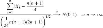
1.12.3
Let Yn = nXn; E{Yn} = ![]() ,
, ![]() . Notice that
. Notice that ![]() iXi −
iXi − ![]() =
= ![]() (Yi−μi), where μi =
(Yi−μi), where μi =![]() = E{Yi}. E|Yi − μi|3 =
= E{Yi}. E|Yi − μi|3 = ![]() . Accordingly,
. Accordingly,
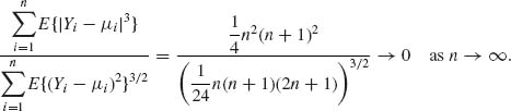
Thus, by Lyapunov’s Theorem,
1.13.5 {Xn} i.i.d. B(1, p), 0 < p < 1.
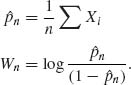
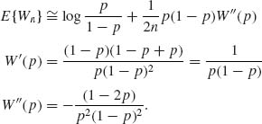
Thus,
![]()
