
CHAPTER 1
Basic Probability Theory
PART I: THEORY
It is assumed that the reader has had a course in elementary probability. In this chapter we discuss more advanced material, which is required for further developments.
1.1 OPERATIONS ON SETS
Let ![]() denote a sample space. Let E1, E2 be subsets of
denote a sample space. Let E1, E2 be subsets of ![]() . We denote the union by E1
. We denote the union by E1 ![]() E2 and the intersection by E1
E2 and the intersection by E1 ![]() E2.
E2. ![]() =
= ![]() − E denotes the complement of E. By DeMorgan’s laws
− E denotes the complement of E. By DeMorgan’s laws ![]() =
= ![]() 1
1 ![]()
![]() 2 and
2 and ![]() =
= ![]() 1
1 ![]()
![]() 2.
2.
Given a sequence of sets {En, n ≥ 1} (finite or infinite), we define
(1.1.1) ![]()
Furthermore, ![]() and
and ![]() are defined as
are defined as
(1.1.2) ![]()
If a point of ![]() belongs to
belongs to ![]() En, it belongs to infinitely many sets En. The sets
En, it belongs to infinitely many sets En. The sets ![]() , En and
, En and ![]() , En always exist and
, En always exist and
(1.1.3) ![]()
If ![]() , En =
, En = ![]() , En, we say that a limit of {En, n ≥ 1} exists. In this case,
, En, we say that a limit of {En, n ≥ 1} exists. In this case,
(1.1.4) ![]()
A sequence {En, n ≥ 1} is called monotone increasing if En ![]() En+1 for all n ≥ 1. In this case
En+1 for all n ≥ 1. In this case ![]() . The sequence is monotone decreasing if En
. The sequence is monotone decreasing if En ![]() En+1, for all n ≥ 1. In this case
En+1, for all n ≥ 1. In this case ![]() . We conclude this section with the definition of a partition of the sample space. A collection of sets
. We conclude this section with the definition of a partition of the sample space. A collection of sets ![]() = {E1, …, Ek} is called a finite partition of
= {E1, …, Ek} is called a finite partition of ![]() if all elements of
if all elements of ![]() are pairwise disjoint and their union is
are pairwise disjoint and their union is ![]() , i.e., Ei
, i.e., Ei ![]() Ej =
Ej = ![]() for all i ≠ j; Ei, Ej
for all i ≠ j; Ei, Ej ![]()
![]() ; and
; and ![]() . If
. If ![]() contains a countable number of sets that are mutually exclusive and
contains a countable number of sets that are mutually exclusive and ![]() , we say that
, we say that ![]() is a countable partition.
is a countable partition.
1.2 ALGEBRA AND σ–FIELDS
Let ![]() be a sample space. An algebra
be a sample space. An algebra ![]() is a collection of subsets of
is a collection of subsets of ![]() satisfying
satisfying
(1.2.1) 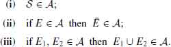
We consider ![]() =
= ![]() . Thus, (i) and (ii) imply that
. Thus, (i) and (ii) imply that ![]()
![]()
![]() . Also, if E1, E2
. Also, if E1, E2 ![]()
![]() then E1
then E1 ![]() E2
E2 ![]()
![]() .
.
The trivial algebra is ![]() 0 = {
0 = {![]() ,
, ![]() }. An algebra
}. An algebra ![]() 1 is a subalgebra of
1 is a subalgebra of ![]() 2 if all sets of
2 if all sets of ![]() 1 are contained in
1 are contained in ![]() 2. We denote this inclusion by
2. We denote this inclusion by ![]() 1
1 ![]()
![]() 2. Thus, the trivial algebra
2. Thus, the trivial algebra ![]() 0 is a subalgebra of every algebra
0 is a subalgebra of every algebra ![]() . We will denote by
. We will denote by ![]() (
(![]() ), the algebra generated by all subsets of
), the algebra generated by all subsets of ![]() (see Example 1.1).
(see Example 1.1).
If a sample space ![]() has a finite number of points n, say 1 ≤ n < ∞, then the collection of all subsets of
has a finite number of points n, say 1 ≤ n < ∞, then the collection of all subsets of ![]() is called the discrete algebra generated by the elementary events of
is called the discrete algebra generated by the elementary events of ![]() . It contains 2n events.
. It contains 2n events.
Let ![]() be a partition of
be a partition of ![]() having k, 2 ≤ k, disjoint sets. Then, the algebra generated by
having k, 2 ≤ k, disjoint sets. Then, the algebra generated by ![]() ,
, ![]() (
(![]() ), is the algebra containing all the 2k − 1 unions of the elements of
), is the algebra containing all the 2k − 1 unions of the elements of ![]() and the empty set.
and the empty set.
An algebra on ![]() is called a σ–field if, in addition to being an algebra, the following holds.
is called a σ–field if, in addition to being an algebra, the following holds.
We will denote a σ–field by ![]() . In a σ–field
. In a σ–field ![]() the supremum, infinum, limsup, and liminf of any sequence of events belong to
the supremum, infinum, limsup, and liminf of any sequence of events belong to ![]() . If
. If ![]() is finite, the discrete algebra
is finite, the discrete algebra ![]() (
(![]() ) is a σ–field. In Example 1.3 we show an algebra that is not a σ–field.
) is a σ–field. In Example 1.3 we show an algebra that is not a σ–field.
The minimal σ–field containing the algebra generated by {(-∞, x], -∞ < x < ∞ } is called the Borel σ–field on the real line ![]() .
.
A sample space ![]() , with a σ–field
, with a σ–field ![]() , (
, (![]() ,
, ![]() ) is called a measurable space.
) is called a measurable space.
The following lemmas establish the existence of smallest σ–field containing a given collection of sets.
Lemma 1.2.1 Let ![]() be a collection of subsets of a sample space
be a collection of subsets of a sample space ![]() . Then, there exists a smallest σ–field
. Then, there exists a smallest σ–field ![]() (
(![]() ), containing the elements of
), containing the elements of ![]() .
.
Proof. The algebra of all subsets of ![]() ,
, ![]() (
(![]() ) obviously contains all elements of
) obviously contains all elements of ![]() . Similarly, the σ–field
. Similarly, the σ–field ![]() containing all subsets of
containing all subsets of ![]() , contains all elements of
, contains all elements of ![]() . Define the σ–field
. Define the σ–field ![]() (
(![]() ) to be the intersection of all σ–fields, which contain all elements of
) to be the intersection of all σ–fields, which contain all elements of ![]() . Obviously,
. Obviously, ![]() (
(![]() ) is an algebra. QED
) is an algebra. QED
A collection ![]() of subsets of
of subsets of ![]() is called a monotonic class if the limit of any monotone sequence in
is called a monotonic class if the limit of any monotone sequence in ![]() belongs to
belongs to ![]() .
.
If ![]() is a collection of subsets of
is a collection of subsets of ![]() , let
, let ![]() * (
* (![]() ) denote the smallest monotonic class containing
) denote the smallest monotonic class containing ![]() .
.
Lemma 1.2.2. A necessary and sufficient condition of an algebra ![]() to be a σ–field is that it is a monotonic class.
to be a σ–field is that it is a monotonic class.
Proof. (i) Obviously, if ![]() is a σ–field, it is a monotonic class.
is a σ–field, it is a monotonic class.
(ii) Let ![]() be a monotonic class.
be a monotonic class.
Let En ![]()
![]() , n ≥ 1. Define
, n ≥ 1. Define ![]() . Obviously Bn
. Obviously Bn ![]() Bn+1 for all n ≥ 1. Hence
Bn+1 for all n ≥ 1. Hence 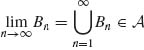 . But
. But ![]() . Thus,
. Thus, ![]() , En
, En ![]()
![]() . Similarly,
. Similarly, ![]() En
En ![]()
![]() . Thus,
. Thus, ![]() is a σ–field. QED
is a σ–field. QED
Theorem 1.2.1. Let ![]() be an algebra. Then
be an algebra. Then ![]() * (
* (![]() ) =
) = ![]() (
(![]() ), where
), where ![]() (
(![]() ) is the smallest σ–field containing
) is the smallest σ–field containing ![]() .
.
Proof. See Shiryayev (1984, p. 139).
The measurable space (![]() ,
, ![]() ), where
), where ![]() is the real line and
is the real line and ![]() =
= ![]() (
(![]() ), called the Borel measurable space, plays a most important role in the theory of statistics. Another important measurable space is (
), called the Borel measurable space, plays a most important role in the theory of statistics. Another important measurable space is (![]() n,
n, ![]() n), n ≥ 2, where
n), n ≥ 2, where ![]() n =
n = ![]() ×
× ![]() × ··· ×
× ··· × ![]() is the Euclidean n–space, and
is the Euclidean n–space, and ![]() n =
n = ![]() × ··· ×
× ··· × ![]() is the smallest σ–field containing
is the smallest σ–field containing ![]() n,
n, ![]() , and all n–dimensional rectangles I = I1 × ··· × In, where
, and all n–dimensional rectangles I = I1 × ··· × In, where
![]()
The measurable space (![]() ∞,
∞, ![]() ∞) is used as a basis for probability models of experiments with infinitely many trials.
∞) is used as a basis for probability models of experiments with infinitely many trials. ![]() ∞ is the space of ordered sequences x = (x1, x2, …), −∞ < xn < ∞, n = 1, 2, …. Consider the cylinder sets
∞ is the space of ordered sequences x = (x1, x2, …), −∞ < xn < ∞, n = 1, 2, …. Consider the cylinder sets
![]()
and
![]()
where Bi are Borel sets, i.e., Bi ![]()
![]() . The smallest σ–field containing all these cylinder sets, n ≥ 1, is
. The smallest σ–field containing all these cylinder sets, n ≥ 1, is ![]() (
(![]() ∞). Examples of Borel sets in
∞). Examples of Borel sets in ![]() (
(![]() ∞) are
∞) are
or
1.3 PROBABILITY SPACES
Given a measurable space (![]() ,
, ![]() ), a probability model ascribes a countably additive function P on
), a probability model ascribes a countably additive function P on ![]() , which assigns a probability P{A} to all sets A
, which assigns a probability P{A} to all sets A ![]()
![]() . This function should satisfy the following properties.
. This function should satisfy the following properties.
(1.3.1) 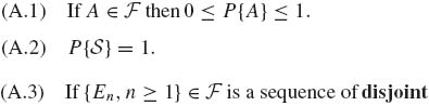
(1.3.2) 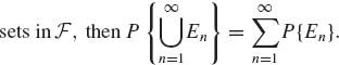
Recall that if A ![]() B then P {A} ≤ P{B}, and P{
B then P {A} ≤ P{B}, and P{![]() } = 1 − P{A}. Other properties will be given in the examples and problems. In the sequel we often write AB for A
} = 1 − P{A}. Other properties will be given in the examples and problems. In the sequel we often write AB for A ![]() B.
B.
Theorem 1.3.1. Let (![]() ,
, ![]() , P) be a probability space, where
, P) be a probability space, where ![]() is a σ–field of subsets of
is a σ–field of subsets of ![]() and P a probability function. Then
and P a probability function. Then
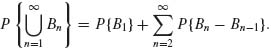
(1.3.4) ![]()
Proof. (i) Since Bn ![]() Bn + 1,
Bn + 1, ![]() . Moreover,
. Moreover,
Notice that for n ≥ 2, since ![]() n Bn−1 =
n Bn−1 = ![]() ,
,
(1.3.6) 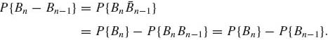
Also, in (1.3.5)
(1.3.7) 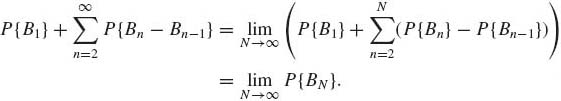
Thus, Equation (1.3.3) is proven.
(ii) Since Bn ![]() Bn + 1, n ≥ 1,
Bn + 1, n ≥ 1, ![]() n
n ![]()
![]() n+1, n ≥ 1.
n+1, n ≥ 1. ![]() . Hence,
. Hence,
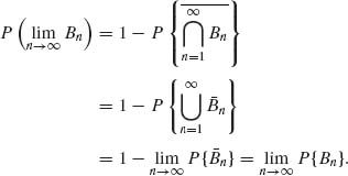 QED
QED
Sets in a probability space are called events.
1.4 CONDITIONAL PROBABILITIES AND INDEPENDENCE
The conditional probability of an event A ![]()
![]() given an event B
given an event B ![]()
![]() such that P {B} > 0, is defined as
such that P {B} > 0, is defined as
(1.4.1) ![]()
We see first that P{· | B} is a probability function on ![]() . Indeed, for every A
. Indeed, for every A ![]()
![]() , 0 ≤ P{A|B} ≤ 1. Moreover, P{
, 0 ≤ P{A|B} ≤ 1. Moreover, P{![]() | B} = 1 and if A1 and A2 are disjoint events in
| B} = 1 and if A1 and A2 are disjoint events in ![]() , then
, then
(1.4.2) 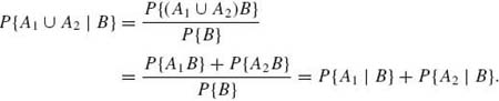
If P{B} > 0 and P{A} ≠ P{A|B}, we say that the events A and B are dependent. On the other hand, if P{A} = P{A|B} we say that A and B are independent events. Notice that two events are independent if and only if
(1.4.3) ![]()
Given n events in ![]() , namely A1, …, An, we say that they are pairwise independent if P{Ai Aj} = P{Ai} P{Aj} for any i ≠ j. The events are said to be independent in triplets if
, namely A1, …, An, we say that they are pairwise independent if P{Ai Aj} = P{Ai} P{Aj} for any i ≠ j. The events are said to be independent in triplets if
![]()
for any i ≠ j≠ k. Example 1.4 shows that pairwise independence does not imply independence in triplets.
Given n events A1, …, An of ![]() , we say that they are independent if, for any 2 ≤ k ≤ n and any k–tuple (1 ≤ i1 < i2 < ··· < ik ≤ n),
, we say that they are independent if, for any 2 ≤ k ≤ n and any k–tuple (1 ≤ i1 < i2 < ··· < ik ≤ n),
(1.4.4) 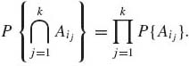
Events in an infinite sequence {A1, A2, … } are said to be independent if {A1, …, An} are independent, for each n ≥ 2. Given a sequence of events A1, A2, … of a σ–field ![]() , we have seen that
, we have seen that
![]()
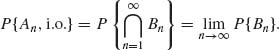
This event means that points w in ![]() , An belong to infinitely many of the events {An}. Thus, the event
, An belong to infinitely many of the events {An}. Thus, the event ![]() , An is denoted also as {An, i.o. }, where i.o. stands for “infinitely often.”
, An is denoted also as {An, i.o. }, where i.o. stands for “infinitely often.”
The following important theorem, known as the Borel–Cantelli Lemma, gives conditions under which P{An, i.o.} is either 0 or 1.
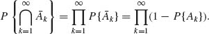
Theorem 1.4.1 (Borel–Cantelli) Let {An} be a sequence of sets in ![]() .
.
Proof. (i) Notice that ![]() is a decreasing sequence. Thus
is a decreasing sequence. Thus
But
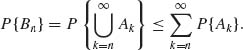
The assumption that ![]() P{An} < ∞ implies that
P{An} < ∞ implies that ![]() P{Ak} = 0.
P{Ak} = 0.
(ii) Since A1, A2, … are independent, ![]() 1,
1, ![]() 2, … are independent. This implies that
2, … are independent. This implies that
If 0 < x ≤ 1 then log (1−x) ≤ −x. Thus,
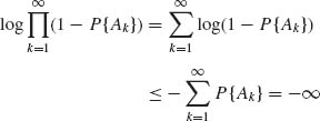
since ![]() P{An} = ∞. Thus
P{An} = ∞. Thus  = 0 for all n ≥ 1. This implies that P{An, i.o.} = 1. QED
We conclude this section with the celebrated Bayes Theorem.
Let ![]() = {Bi, i
= {Bi, i ![]() J} be a partition of
J} be a partition of ![]() , where J is an index set having a finite or countable number of elements. Let Bj
, where J is an index set having a finite or countable number of elements. Let Bj ![]()
![]() and P{Bj} > 0 for all j
and P{Bj} > 0 for all j ![]() J. Let A
J. Let A ![]()
![]() , P{A} > 0. We are interested in the conditional probabilities P{Bj| A}, j
, P{A} > 0. We are interested in the conditional probabilities P{Bj| A}, j ![]() J.
J.
Theorem 1.4.2 (Bayes).
(1.4.5) 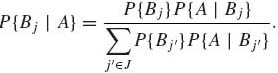
Proof. Left as an exercise. QED
Bayes Theorem is widely used in scientific inference. Examples of the application of Bayes Theorem are given in many elementary books. Advanced examples of Bayesian inference will be given in later chapters.
1.5 RANDOM VARIABLES AND THEIR DISTRIBUTIONS
Random variables are finite real value functions on the sample space ![]() , such that measurable subsets of
, such that measurable subsets of ![]() are mapped into Borel sets on the real line and thus can be assigned probability measures. The situation is simple if
are mapped into Borel sets on the real line and thus can be assigned probability measures. The situation is simple if ![]() contains only a finite or countably infinite number of points.
contains only a finite or countably infinite number of points.
In the general case, ![]() might contain non–countable infinitely many points. Even if
might contain non–countable infinitely many points. Even if ![]() is the space of all infinite binary sequences w = (i1, i2, …), the number of points in
is the space of all infinite binary sequences w = (i1, i2, …), the number of points in ![]() is non–countable. To make our theory rich enough, we will require that the probability space will be (
is non–countable. To make our theory rich enough, we will require that the probability space will be (![]() ,
, ![]() , P), where
, P), where ![]() is a σ–field. A random variable X is a finite real value function on
is a σ–field. A random variable X is a finite real value function on ![]() . We wish to define the distribution function of X, on
. We wish to define the distribution function of X, on ![]() , as
, as
For this purpose, we must require that every Borel set on ![]() has a measurable inverse image with respect to
has a measurable inverse image with respect to ![]() . More specifically, given (
. More specifically, given (![]() ,
, ![]() , P), let (
, P), let (![]() ,
, ![]() ) be Borel measurable space where
) be Borel measurable space where ![]() is the real line and
is the real line and ![]() the Borel σ–field of subsets of
the Borel σ–field of subsets of ![]() . A subset of (
. A subset of (![]() , B) is called a Borel set if B belongs to
, B) is called a Borel set if B belongs to ![]() . Let X:
. Let X: ![]() →
→ ![]() . The inverse image of a Borel set B with respect to X is
. The inverse image of a Borel set B with respect to X is
(1.5.2) ![]()
A function X: ![]() →
→ ![]() is called
is called ![]() –measurable if X−1 (B)
–measurable if X−1 (B) ![]()
![]() for all B
for all B ![]()
![]() . Thus, a random variable with respect to (
. Thus, a random variable with respect to (![]() ,
, ![]() , P) is an
, P) is an ![]() –measurable function on
–measurable function on ![]() . The class
. The class ![]() X = {X−1(B): B
X = {X−1(B): B ![]()
![]() } is also a σ–field, generated by the random variable X. Notice that
} is also a σ–field, generated by the random variable X. Notice that ![]() X
X ![]()
![]() .
.
By definition, every random variable X has a distribution function FX. The probability measure PX{·} induced by X on (![]() , B) is
, B) is
(1.5.3) ![]()
A distribution function FX is a real value function satisfying the properties
Thus, a distribution function F is right–continuous.
Given a distribution function FX, we obtain from (1.5.1), for every −∞ < a < b < ∞,
(1.5.4) ![]()
and
(1.5.5) ![]()
Thus, if FX is continuous at a point x0, then P{w: X(w) = x0} = 0. If X is a random variable, then Y = g(X) is a random variable only if g is ![]() –(Borel) measurable, i.e., for any B
–(Borel) measurable, i.e., for any B ![]()
![]() , g−1 (B)
, g−1 (B) ![]()
![]() . Thus, if Y = g(X), g is
. Thus, if Y = g(X), g is ![]() –measurable and X
–measurable and X ![]() –measurable, then Y is also
–measurable, then Y is also ![]() –measurable. The distribution function of Y is
–measurable. The distribution function of Y is
(1.5.6) ![]()
Any two random variables X, Y having the same distribution are equivalent. We denote this by Y ~ X.
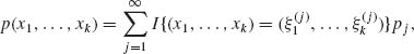
A distribution function F may have a countable number of distinct points of discontinuity. If x0 is a point of discontinuity, F(x0) − F(x0−) > 0. In between points of discontinuity, F is continuous. If F assumes a constant value between points of discontinuity (step function), it is called discrete. Formally, let −∞ < x1 < x2 < ··· < ∞ be points of discontinuity of F. Let IA(x) denote the indicator function of a set A, i.e.,
![]()
Then a discrete F can be written as
(1.5.7) 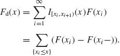
Let μ1 and μ2 be measures on (![]() ,
, ![]() ). We say that μ1 is absolutely continuous with respect to μ2, and write μ1
). We say that μ1 is absolutely continuous with respect to μ2, and write μ1 ![]() μ2, if B
μ2, if B ![]()
![]() and μ2 (B) = 0 then μ1(B) = 0. Let λ denote the Lebesgue measure on (
and μ2 (B) = 0 then μ1(B) = 0. Let λ denote the Lebesgue measure on (![]() ,
, ![]() ). For every interval (a, b], −∞ < a < b < ∞, λ ((a, b]) = b−a. The celebrated Radon–Nikodym Theorem (see Shiryayev, 1984, p. 194) states that if μ1
). For every interval (a, b], −∞ < a < b < ∞, λ ((a, b]) = b−a. The celebrated Radon–Nikodym Theorem (see Shiryayev, 1984, p. 194) states that if μ1 ![]() μ2 and μ1, μ2 are σ–finite measures on (
μ2 and μ1, μ2 are σ–finite measures on (![]() ,
, ![]() ), there exists a
), there exists a ![]() –measurable nonnegative function f(x) so that, for each B
–measurable nonnegative function f(x) so that, for each B ![]()
![]() ,
,
where the Lebesgue integral in (1.5.8) will be discussed later. In particular, if Pc is absolutely continuous with respect to the Lebesgue measure λ, then there exists a function f ≥ 0 so that
(1.5.9) ![]()
Moreover,
(1.5.10) ![]()
A distribution function F is called absolutely continuous if there exists a nonnegative function f such that
(1.5.11) 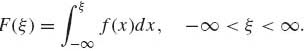
The function f, which can be represented for “almost all x” by the derivative of F, is called the probability density function (p.d.f.) corresponding to F.
If F is absolutely continuous, then f(x) = ![]() F(x) “almost everywhere.” The term “almost everywhere” or “almost all” x means for all x values, excluding maybe on a set N of Lebesgue measure zero. Moreover, the probability assigned to any interval (α, β], α ≤ β, is
F(x) “almost everywhere.” The term “almost everywhere” or “almost all” x means for all x values, excluding maybe on a set N of Lebesgue measure zero. Moreover, the probability assigned to any interval (α, β], α ≤ β, is
(1.5.12) ![]()
Due to the continuity of F we can also write
![]()
Often the density functions f are Riemann integrable, and the above integrals are Riemann integrals. Otherwise, these are all Lebesgue integrals, which are defined in the next section.
There are continuous distribution functions that are not absolutely continuous. Such distributions are called singular. An example of a singular distribution is the Cantor distribution (see Shiryayev, 1984, p. 155).
Finally, every distribution function F(x) is a mixture of the three types of distributions—discrete distribution Fd(·), absolutely continuous distributions Fac(·), and singular distributions Fs(·). That is, for some 0 ≤ p1, p2, p3 ≤ 1 such that p1 + p2 + p3 = 1,
![]()
In this book we treat only mixtures of Fd(x) and Fac(x).
1.6 THE LEBESGUE AND STIELTJES INTEGRALS
1.6.1 General Definition of Expected Value: The Lebesgue Integral
Let (![]() ,
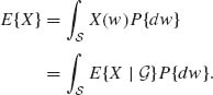
, ![]() , P) be a probability space. If X is a random variable, we wish to define the integral
, P) be a probability space. If X is a random variable, we wish to define the integral
(1.6.1) ![]()
We define first E{X} for nonnegative random variables, i.e., X(w) ≥ 0 for all w ![]()
![]() . Generally, X = X+ − X−, where X+ (w) = max (0, X(w)) and X−(w) = −min (0, X(w)).
. Generally, X = X+ − X−, where X+ (w) = max (0, X(w)) and X−(w) = −min (0, X(w)).
Given a nonnegative random variable X we construct for a given finite integer n the events
![]()
and
![]()
These events form a partition of ![]() . Let Xn, n ≥ 1, be the discrete random variable defined as
. Let Xn, n ≥ 1, be the discrete random variable defined as
(1.6.2) 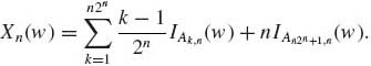
Notice that for each w, Xn (w) ≤ Xn+1(w) ≤ … ≤ X(w) for all n. Also, if w ![]() Ak, n, k = 1, …, n2n, then |X(w) − Xn(w)| ≤
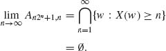
Ak, n, k = 1, …, n2n, then |X(w) − Xn(w)| ≤ ![]() . Moreover, An2n+1, n
. Moreover, An2n+1, n ![]() A(n+1)2n+1, n+1, all n ≥ 1. Thus
A(n+1)2n+1, n+1, all n ≥ 1. Thus
Thus for all w ![]()
![]()
(1.6.3) ![]()
Now, for each discrete random variable Xn(w)
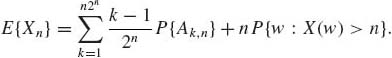
Obviously E {Xn} ≤ n, and E{Xn+1} ≥ E{Xn}. Thus, ![]() E{Xn} exists (it might be +∞). Accordingly, the Lebesgue integral is defined as
E{Xn} exists (it might be +∞). Accordingly, the Lebesgue integral is defined as
(1.6.5) 
The Lebesgue integral may exist when the Riemann integral does not. For example, consider the probability space (![]() ,
, ![]() , P) where
, P) where ![]() = {x: 0 ≤ x ≤ 1},
= {x: 0 ≤ x ≤ 1}, ![]() the Borel σ–field on
the Borel σ–field on ![]() , and P the Lebesgue measure on [
, and P the Lebesgue measure on [![]() ]. Define
]. Define
![]()
Let B0 = {x: 0 ≤ x ≤ 1, f(x) = 0}, B1 = [0, 1]− B0. The Lebesgue integral of f is
![]()
since the Lebesgue measure of B1 is zero. On the other hand, the Riemann integral of f(x) does not exist. Notice that, contrary to the construction of the Riemann integral, the Lebesgue integral ![]() f(x)P{dx} of a nonnegative function f is obtained by partitioning the range of the function f to 2n subintervals
f(x)P{dx} of a nonnegative function f is obtained by partitioning the range of the function f to 2n subintervals ![]() n = {
n = {![]() } and constructing a discrete random variable
} and constructing a discrete random variable ![]() =
= ![]() I{x
I{x ![]()
![]() }, where fn, j = inf{f(x): x
}, where fn, j = inf{f(x): x ![]()
![]() }. The expected value of
}. The expected value of ![]() is E{
is E{![]() } =
} = ![]() P(X
P(X ![]()
![]() ). The sequence {E{
). The sequence {E{![]() }, n≥ 1} is nondecreasing, and its limit exists (might be +∞). Generally, we define
}, n≥ 1} is nondecreasing, and its limit exists (might be +∞). Generally, we define
(1.6.6) ![]()
if either E{X+} < ∞ or E{X−} < ∞.
If E{X+} = ∞ and E{X−} = ∞, we say that E{X} does not exist. As a special case, if F is absolutely continuous with density f, then
![]()
provided ![]() |x| f>(x)dx < ∞. If F is discrete then
|x| f>(x)dx < ∞. If F is discrete then
![]()
provided it is absolutely convergent.
From the definition (1.6.4), it is obvious that if P{X(w) ≥ 0} = 1 then E{X} ≥ 0. This immediately implies that if X and Y are two random variables such that P{w: X(w) ≥ Y(w)} = 1, then E{X−Y} ≥ 0. Also, if E{X} exists then, for all A ![]()
![]() ,
,
![]()
and E{XIA(X)} exists. If E{X} is finite, E{XIA(X)} is also finite. From the definition of expectation we immediately obtain that for any finite constant c,
Equation (1.6.7) implies that the expected value is a linear functional, i.e., if X1, …, Xn are random variables on (![]() ,
, ![]() , P) and β0, β1, …, βn are finite constants, then, if all expectations exist,
, P) and β0, β1, …, βn are finite constants, then, if all expectations exist,
(1.6.8) 
We present now a few basic theorems on the convergence of the expectations of sequences of random variables.
Theorem 1.6.1 (Monotone Convergence) Let {Xn} be a monotone sequence of random variables and Y a random variable.
![]()
![]()
Proof. See Shiryayev (1984, p. 184). QED
Corollary 1.6.1. If X1, X2, … are nonnegative random variables, then
(1.6.9) 
Theorem 1.6.2. (Fatou) Let Xn, n ≥ 1 and Y be random variables.
![]()
![]()
(1.6.10) ![]()
Proof. (i)
![]()
The sequence Zn(w) = ![]() Xm(w), n ≥ 1 is monotonically increasing for each w, and Zn(w) ≥ Y(w), n ≥ 1. Hence, by Theorem 1.6.1,
Xm(w), n ≥ 1 is monotonically increasing for each w, and Zn(w) ≥ Y(w), n ≥ 1. Hence, by Theorem 1.6.1,
![]()
Or
![]()
The proof of (ii) is obtained by defining Zn(w) = ![]() Xm(w), and applying the previous theorem. Part (iii) is a result of (i) and (ii). QED
Xm(w), and applying the previous theorem. Part (iii) is a result of (i) and (ii). QED
Theorem 1.6.3. (Lebesgue Dominated Convergence) Let Y, X, Xn, n ≥ 1, be random variables such that |Xn(w)| ≤ Y(w), n ≥ 1 for almost all w, and E{Y} < ∞. Assume also that P![]() . Then E{|X|} < ∞ and
. Then E{|X|} < ∞ and
(1.6.11) ![]()
and
(1.6.12) ![]()
Proof. By Fatou’s Theorem (Theorem 1.6.2)
![]()
But since ![]() Xn(w) = X(w), with probability 1,
Xn(w) = X(w), with probability 1,
![]()
Moreover, |X(w)| < Y(w) for almost all w (with probability 1). Hence, E{|X|} < ∞. Finally, since |Xn(w) − X(w)| ≤ 2Y(w), with probability 1
![]() QED
QED
We conclude this section with a theorem on change of variables under Lebesgue integrals.
Theorem 1.6.4 Let X be a random variable with respect to (![]() ,
, ![]() , P). Let g:
, P). Let g: ![]() →
→ ![]() be a Borel measurable function. Then for each B
be a Borel measurable function. Then for each B ![]()
![]() ,
,
The proof of the theorem is based on the following steps.
1.6.2 The Stieltjes–Riemann Integral
Let g be a function of a real variable and F a distribution function. Let (α, β] be a half–closed interval. Let
![]()
be a partition of (α, β] to n subintervals (xi−1, xi], i = 1, …, n. In each subinterval choose x’i, xi−1 < x’i ≤ xi and consider the sum
(1.6.14) 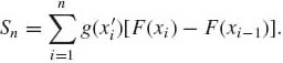
If, as n → ∞, ![]() |xi − xi−1| → 0 and if
|xi − xi−1| → 0 and if ![]() Sn exists (finite) independently of the partitions, then the limit is called the Stieltjes–Riemann integral of g with respect to F. We denote this integral as
Sn exists (finite) independently of the partitions, then the limit is called the Stieltjes–Riemann integral of g with respect to F. We denote this integral as
![]()
This integral has the usual linear properties, i.e.,
(1.6.15) ![]()
and
One can integrate by parts, if all expressions exist, according to the formula
(1.6.16) ![]()
where g’(x) is the derivative of g(x). If F is strictly discrete, with jump points −∞ < ξ1 < ξ2 < ··· <∞,
(1.6.17) 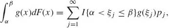
where pj = F(ξj) − F(ξj−), j = 1, 2, …. If F is absolutely continuous, then at almost all points,
![]()
as dx → 0. Thus, in the absolutely continuous case
(1.6.18) 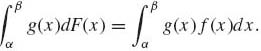
Finally, the improper Stieltjes–Riemann integral, if it exists, is
(1.6.19) 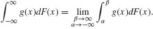
If B is a set obtained by union and complementation of a sequence of intervals, we can write, by setting g(x) = I{x ![]() B},
B},
(1.6.20) 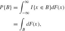
where F is either discrete or absolutely continuous.
1.6.3 Mixtures of Discrete and Absolutely Continuous Distributions
Let Fd be a discrete distribution and let Fac be an absolutely continuous distribution function. Then for all α 0 ≤ α ≤ 1,
(1.6.21) ![]()
is also a distribution function, which is a mixture of the two types. Thus, for such mixtures, if −∞ < ξ1 < ξ2 < ··· < ∞ are the jump points of Fd, then for every −∞ < γ ≤ δ < ∞ and B = (γ, δ],
(1.6.22) 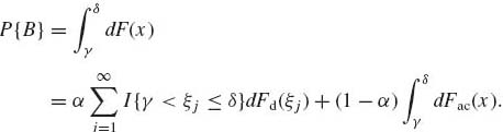
Moreover, if B+ = [γ, δ] then
![]()
The expected value of X, when F(x) = pFd(x) + (1−p) Fac(x) is,
(1.6.23) 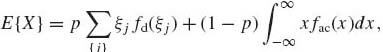
where {ξj} is the set of jump points of Fd; fd and fac are the corresponding p.d.f.s. We assume here that the sum and the integral are absolutely convergent.
1.6.4 Quantiles of Distributions
The p–quantiles or fractiles of distribution functions are inverse points of the distributions. More specifically, the p–quantile of a distribution function F, designated by xp or F−1(p), is the smallest value of x at which F(x) is greater or equal to p, i.e.,
(1.6.24) ![]()
The inverse function defined in this fashion is unique. The median of a distribution, x.5, is an important parameter characterizing the location of the distribution. The lower and upper quartiles are the .25– and .75–quantiles. The difference between these quantiles, RQ = x.75 − x.25, is called the interquartile range. It serves as one of the measures of dispersion of distribution functions.
1.6.5 Transformations
From the distribution function F(x) = α Fd(x) + (1−α) Fac(x), 0 ≤ α ≤ 1, we can derive the distribution function of a transformed random variable Y = g(X), which is
(1.6.25) 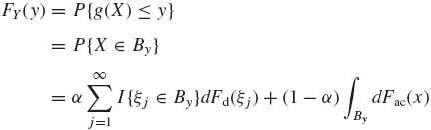
where
![]()
In particular, if F is absolutely continuous and if g is a strictly increasing differentiable function, then the p.d.f. of Y, h(y), is
(1.6.26) ![]()
where g−1(y) is the inverse function. If g’(x) < 0 for all x, then
(1.6.27) 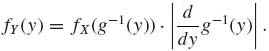
Suppose that X is a continuous random variable with p.d.f. f(x). Let g(x) be a differentiable function that is not necessarily one–to–one, like g(x) = x2. Excluding cases where g(x) is a constant over an interval, like the indicator function, let m(y) denote the number of roots of the equation g(x) = y. Let ξj(y), j = 1, …, m(y) denote the roots of this equation. Then the p.d.f. of Y = g(x) is
(1.6.28) 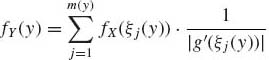
if m(y) > 0 and zero otherwise.
1.7 JOINT DISTRIBUTIONS, CONDITIONAL DISTRIBUTIONS AND INDEPENDENCE
1.7.1 Joint Distributions
Let (X1, …, Xk) be a vector of k random variables defined on the same probability space. These random variables represent variables observed in the same experiment. The joint distribution function of these random variables is a real value function F of k real arguments (ξ1, …, ξk) such that
(1.7.1) ![]()
The joint distribution of two random variables is called a bivariate distribution function.
Every bivariate distribution function F has the following properties.
(1.7.2) 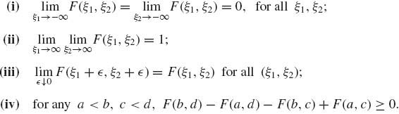
Property (iii) is the right continuity of F(ξ1, ξ2). Property (iv) means that the probability of every rectangle is nonnegative. Moreover, the total increase of F(ξ1, ξ2) is from 0 to 1. The similar properties are required in cases of a larger number of variables.
Given a bivariate distribution function F. The univariate distributions of X1 and X2 are F1 and F2 where
(1.7.3) ![]()
F1 and F2 are called the marginal distributions of X1 and X2, respectively. In cases of joint distributions of three variables, we can distinguish between three marginal bivariate distributions and three marginal univariate distributions. As in the univariate case, multivariate distributions are either discrete, absolutely continuous, singular, or mixtures of the three main types. In the discrete case there are at most a countable number of points {(![]() , …,
, …, ![]() ), j = 1, 2, … } on which the distribution concentrates. In this case the joint probability function is
), j = 1, 2, … } on which the distribution concentrates. In this case the joint probability function is
(1.7.4) 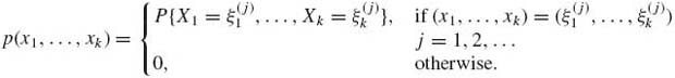
Such a discrete p.d.f. can be written as
where pj = P{X1 =![]() , …, Xk =
, …, Xk = ![]() }.
}.
In the absolutely continuous case there exists a nonnegative function f(x1, …, xk) such that
(1.7.5) 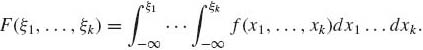
The function f(x1, …, xk) is called the joint density function.
The marginal probability or density functions of single variables or of a subvector of variables can be obtained by summing (in the discrete case) or integrating, in the absolutely continuous case, the joint distribution functions (densities) with respect to the variables that are not under consideration, over their range of variation.
Although the presentation here is in terms of k discrete or k absolutely continuous random variables, the joint distributions can involve some discrete and some continuous variables, or mixtures.
If X1 has an absolutely continuous marginal distribution and X2 is discrete, we can introduce the function N(B) on ![]() , which counts the number of jump points of X2 that belong to B. N(B) is a σ–finite measure. Let λ (B) be the Lebesgue measure on
, which counts the number of jump points of X2 that belong to B. N(B) is a σ–finite measure. Let λ (B) be the Lebesgue measure on ![]() . Consider the σ–finite measure on
. Consider the σ–finite measure on ![]() (2), μ (B1×B2) = λ (B1)N(B2). If X1 is absolutely continuous and X2 discrete, their joint probability measure PX is absolutely continuous with respect to μ. There exists then a nonnegative function fX such that
(2), μ (B1×B2) = λ (B1)N(B2). If X1 is absolutely continuous and X2 discrete, their joint probability measure PX is absolutely continuous with respect to μ. There exists then a nonnegative function fX such that
![]()
The function fX is a joint p.d.f. of X1, X2 with respect to μ. The joint p.d.f. fX is positive only at jump point of X2.
If X1, …, Xk have a joint distribution with p.d.f. f(x1, …, xk), the expected value of a function g(X1, …, Xk) is defined as
(1.7.6) ![]()
We have used here the conventional notation for Stieltjes integrals.
Notice that if (X, Y) have a joint distribution function F(x, y) and if X is discrete with jump points of F1(x) at ξ1, ξ2, …, and Y is absolutely continuous, then, as in the previous example,
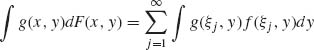
where f(x, y) is the joint p.d.f. A similar formula holds for the case of X, absolutely continuous and Y, discrete.
1.7.2 Conditional Expectations: General Definition
Let X(w) ≥ 0, for all w ![]()
![]() , be a random variable with respect to (
, be a random variable with respect to (![]() ,
, ![]() , P). Consider a σ–field
, P). Consider a σ–field ![]() ,
, ![]()
![]()
![]() . The conditional expectation of X given
. The conditional expectation of X given ![]() is defined as a
is defined as a ![]() –measurable random variable E{X|
–measurable random variable E{X| ![]() } satisfying
} satisfying
for all A ![]()
![]() . Generally, E{X|
. Generally, E{X| ![]() } is defined if min {E{X+|
} is defined if min {E{X+| ![]() }, E{X−|
}, E{X−| ![]() }} < ∞ and E{X|
}} < ∞ and E{X| ![]() } = E{X+|
} = E{X+| ![]() } − E{X−|
} − E{X−| ![]() }. To see that such conditional expectations exist, where X(w) ≥ 0 for all w, consider the σ–finite measure on
}. To see that such conditional expectations exist, where X(w) ≥ 0 for all w, consider the σ–finite measure on ![]() ,
,
(1.7.8) ![]()
Obviously Q ![]() P and by Radon–Nikodym Theorem, there exists a nonnegative,
P and by Radon–Nikodym Theorem, there exists a nonnegative, ![]() –measurable random variable E{X|
–measurable random variable E{X| ![]() } such that
} such that
(1.7.9) ![]()
According to the Radon–Nikodym Theorem, E{X| ![]() } is determined only up to a set of P–measure zero.
} is determined only up to a set of P–measure zero.
If B ![]()
![]() and X(w) = IB(w), then E{X|
and X(w) = IB(w), then E{X| ![]() } = P{B|
} = P{B| ![]() } and according to (1.6.13),
} and according to (1.6.13),
(1.7.10) 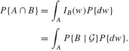
Notice also that if X is ![]() –measurable then X = E{X|
–measurable then X = E{X| ![]() } with probability 1.
} with probability 1.
On the other hand, if ![]() = {
= {![]() ,
, ![]() } is the trivial algebra, then E{X|
} is the trivial algebra, then E{X| ![]() } = E{X} with probability 1.
} = E{X} with probability 1.
From the definition (1.7.7), since ![]()
![]()
![]() ,
,
This is the law of iterated expectation; namely, for all ![]()
![]()
![]() ,
,
(1.7.11) ![]()
Furthermore, if X and Y are two random variables on (![]() ,
, ![]() , P), the collection of all sets {Y−1 (B), B
, P), the collection of all sets {Y−1 (B), B ![]()
![]() }, is a σ–field generated by Y. Let
}, is a σ–field generated by Y. Let ![]() Y denote this σ–field. Since Y is a random variable,
Y denote this σ–field. Since Y is a random variable, ![]() Y
Y ![]()
![]() . We define
. We define
Let y0 be such that fY(y0) > 0.
Consider the ![]() Y–measurable set Aδ = {w: y0 < Y(w) ≤ y0 + δ }. According to (1.7.7)
Y–measurable set Aδ = {w: y0 < Y(w) ≤ y0 + δ }. According to (1.7.7)
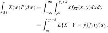
The left–hand side of (1.7.13) is, if E{|X|} <∞,
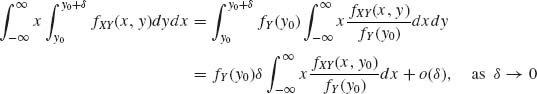
where ![]() = 0. The right–hand side of (1.7.13) is
= 0. The right–hand side of (1.7.13) is
![]()
Dividing both sides of (1.7.13) by fY(y0)δ, we obtain that
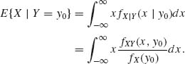
We therefore define for fY(y0) > 0
(1.7.14) ![]()
More generally, for k > 2 let f(x1, …, xk) denote the joint p.d.f. of (X1, …, Xk). Let 1 ≤ r < k and g(x1, …, xr) denote the marginal joint p.d.f. of (X1, …, Xr). Suppose that (ξ1, …, ξr) is a point at which g(ξ1, …, ξr) > 0. The conditional p.d.f. of Xr+1, …, Xk given {X1 = ξ1, …, Xr = ξr} is defined as
(1.7.15) ![]()
We remark that conditional distribution functions are not defined on points (ξ1, …, ξr) such that g(ξ1, …, ξr) = 0. However, it is easy to verify that the probability associated with this set of points is zero. Thus, the definition presented here is sufficiently general for statistical purposes. Notice that f(xr+1, …, xk | ξ1, …, ξr) is, for a fixed point (ξ1, …, ξr) at which it is well defined, a nonnegative function of (xr+1, …, xk) and that
![]()
Thus, f(xr+1, …, xk| ξ1, …, ξr) is indeed a joint p.d.f. of (Xr+1, …, Xk). The point (ξ1, …, ξr) can be considered a parameter of the conditional distribution.
If ![]() (Xr+1, …, Xk) is an (integrable) function of (Xr+1, …, Xk), the conditional expectation of
(Xr+1, …, Xk) is an (integrable) function of (Xr+1, …, Xk), the conditional expectation of ![]() (Xr+1, …, Xk) given {X1 = ξ1, …, Xr = ξr} is
(Xr+1, …, Xk) given {X1 = ξ1, …, Xr = ξr} is
(1.7.16) ![]()
This conditional expectation exists if the integral is absolutely convergent.
1.7.3 Independence
Random variables X1, …, Xn, on the same probability space, are called mutually independent if, for any Borel sets B1, …, Bn,
(1.7.17) 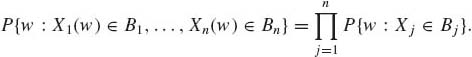
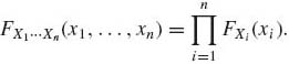
Accordingly, the joint distribution function of any k–tuple (Xi1, …, Xik) is a product of their marginal distributions. In particular,
Equation (1.7.18) implies that if X1, …, Xn have a joint p.d.f. fX(x1, …, xn) and if they are independent, then
(1.7.19) 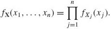
Moreover, if g(X1, …, Xn) = ![]() gj(Xj), where g(x1, …, xn) is
gj(Xj), where g(x1, …, xn) is ![]() (n)–measurable and gj(x) are
(n)–measurable and gj(x) are ![]() –measurable, then under independence
–measurable, then under independence
(1.7.20) 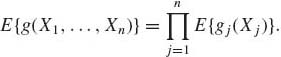
Probability models with independence structure play an important role in statistical theory. From (1.7.12) and (1.7.21), we imply that if X(r) = (X1, …, Xr) and Y(r) = (Xr+1, …, Xn) are independent subvectors, then the conditional distribution of X(r) given Y(r) is independent of Y(r), i.e.,
with probability one.
1.8 MOMENTS AND RELATED FUNCTIONALS
A moment of order r, r = 1, 2, …, of a distribution F(x) is
(1.8.1) ![]()
The moments of Y = X − μ1 are called central moments and those of |X| are called absolute moments. It is simple to prove that the existence of an absolute moment of order r, r > 0, implies the existence of all moments of order s, 0 < s ≤ r, (see Section 1.13.3).
Let μ* r = E{(X − μ1)r}, r = 1, 2, … denote the rth central moment of a distribution. From the binomial expansion and the linear properties of the expectation operator we obtain the relationship between moments (about the origin) μr and center moments mr
(1.8.2) 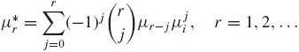
where μ0 ≡ 1.
A distribution function F is called symmetric about a point ξ0 if its p.d.f. is symmetric about ξ0, i.e.,
![]()
From this definition we immediately obtain the following results.
The central moment of the second order occupies a central role in the theory of statistics and is called the variance of X. The variance is denoted by V{X}. The square–root of the variance, called the standard deviation, is a measure of dispersion around the expected value. We denote the standard deviation by σ. The variance of X is equal to
(1.8.3) ![]()
The variance is always nonnegative, and hence for every distribution having a finite second moment E{X2} ≥ (E{X})2. One can easily verify from the definition that if X is a random variable and a and b are constants, then V{a + bX} = b2V{X}.
The variance is equal to zero if and only if the distribution function is concentrated at one point (a degenerate distribution).
A famous inequality, called the Chebychev inequality, relates the probability of X concentrating around its mean, and the standard deviation σ.
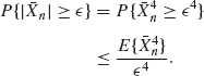
Theorem 1.8.1. (Chebychev) If FX has a finite standard deviation σ, then, for every a > 0,
(1.8.4) ![]()
where μ = E{X}.
Proof.
(1.8.5) 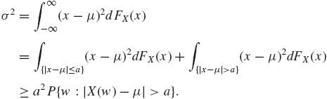
Hence,
![]() QED
QED
Notice that in the proof of the theorem, we used the Riemann–Stieltjes integral. The theorem is true for any type of distribution for which 0 ≤ σ < ∞. The Chebychev inequality is a crude inequality. Various types of better inequalities are available, under additional assumptions (see Zelen and Severv, 1968; Rohatgi, 1976, p. 102).
The moment generating function (m.g.f.) of a random variable X, denoted by M, is defined as
(1.8.6) ![]()
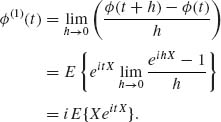
where t is such that M(t) < ∞. Obviously, at t = 0, M(0) = 1. However, M(t) may not exist when t ≠ 0. Assume that M(t) exists for all t in some interval (a, b), a < 0 < b. There is a one–to–one correspondence between the distribution function F and the moment generating function M. M is analytic on (a, b), and can be differentiated under the expectation integral. Thus
(1.8.7) ![]()
Under this assumption the rth derivative of M(t) evaluated at t = 0 yields the moment of order r.
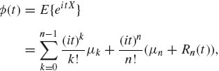
To overcome the problem of M being undefined in certain cases, it is useful to use the characteristic function
(1.8.8) ![]()
where i = ![]() . The characteristic function exists for all t since
. The characteristic function exists for all t since
(1.8.9) ![]()
Indeed, |eitx| = 1 for all x and all t.
If X assumes nonnegative integer values, it is often useful to use the probability generating function (p.g.f.)
(1.8.10) 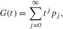
which is convergent if |t| < 1. Moreover, given a p.g.f. of a nonnegative integer value random variable X, its p.d.f. can be obtained by the formula
(1.8.11) ![]()
The logarithm of the moment generating function is called cumulants generating function. We denote this generating function by K. K exists for all t for which M is finite. Both M and K are analytic functions in the interior of their domains of convergence. Thus we can write for t close to zero
(1.8.12) 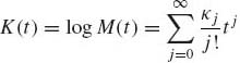
The coefficients {κj} are called cumulants. Notice that κ0 = 0, and κj, j ≥ 1, can be obtained by differentiating K(t) j times, and setting t = 0. Generally, the relationships between the cumulants and the moments of a distribution are, for j =1, …, 4
(1.8.13) 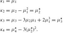
The following two indices
(1.8.14) ![]()
and
(1.8.15) ![]()
where σ2 = ![]() is the variance, are called coefficients of skewness (asymmetry) and kurtosis (steepness), respectively. If the distribution is symmetric, then β1 = 0. If β1 > 0 we say that the distribution is positively skewed; if β1 < 0, it is negatively skewed. If β2 > 3 we say that the distribution is steep, and if β2 < 3 we say that the distribution is flat.
is the variance, are called coefficients of skewness (asymmetry) and kurtosis (steepness), respectively. If the distribution is symmetric, then β1 = 0. If β1 > 0 we say that the distribution is positively skewed; if β1 < 0, it is negatively skewed. If β2 > 3 we say that the distribution is steep, and if β2 < 3 we say that the distribution is flat.
The following equation is called the law of total variance.
If E{X2} < ∞ then
where V{X | Y} denotes the conditional variance of X given Y.
It is often the case that it is easier to find the conditional mean and variance, E{X | Y} and V{X | Y}, than to find E{X} and V{X} directly. In such cases, formula (1.8.16) becomes very handy.
The product central moment of two variables (X, Y) is called the covariance and denoted by cov (X, Y). More specifically
(1.8.17) 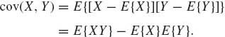
Notice that cov (X, Y) = cov(Y, X), and cov(X, X) = V{X}. Notice that if X is a random variable having a finite first moment and a is any finite constant, then cov(a, X) = 0. Furthermore, whenever the second moments of X and Y exist the covariance exists. This follows from the Schwarz inequality (see Section 1.13.3), i.e., if F is the joint distribution of (X, Y) and FX, FY are the marginal distributions of X and Y, respectively, then
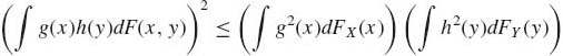
whenever E{g2(X)} and E{h2(Y)} are finite. In particular, for any two random variables having second moments
![]()
The ratio
(1.8.19) ![]()
is called the coefficient of correlation (Pearson’s product moment correlation). From (1.8.18) we deduce that −1 ≤ ρ ≤ 1. The sign of ρ is that of cov(X, Y).
The m.g.f. of a multivariate distribution is a function of k variables
(1.8.20) 
Let X1, …, Xk be random variables having a joint distribution. Consider the linear transformation Y = ![]() βj Xj, where β1, …, βk are constants. Some formulae for the moments and covariances of such linear functions are developed here. Assume that all the moments under consideration exist. Starting with the expected value of Y we prove:
βj Xj, where β1, …, βk are constants. Some formulae for the moments and covariances of such linear functions are developed here. Assume that all the moments under consideration exist. Starting with the expected value of Y we prove:
(1.8.21) 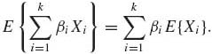
This result is a direct implication of the definition of the integral as a linear operator.
Let X denote a random vector in a column form and X’ its transpose. The expected value of a random vector X’ = (X1, …, Xk) is defined as the corresponding vector of expected values, i.e.,
(1.8.22) ![]()
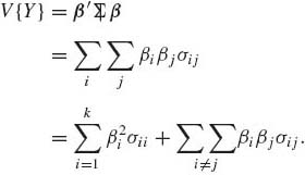
Furthermore, let ![]() denote a k × k matrix with elements that are the variances and covariances of the components of X. In symbols
denote a k × k matrix with elements that are the variances and covariances of the components of X. In symbols
(1.8.23) ![]()
where σij = cov(Xi, Xj), σii = V{Xi}. If Y = β’X where β is a vector of constants, then
The result given by (1.8.24) can be generalized in the following manner. Let Y1 = β’ X and Y2 = α’ X, where α and β are arbitrary constant vectors. Then
(1.8.25) ![]()
Finally, if X is a k–dimensional random vector with covariance matrix ![]() and Y is an m–dimensional vector Y = A X, where A is an m × k matrix of constants, then the covariance matrix of Y is
and Y is an m–dimensional vector Y = A X, where A is an m × k matrix of constants, then the covariance matrix of Y is
(1.8.26) ![]()
In addition, if the covariance matrix of X is ![]() , then the covariance matrix of Y = ξ + AX is V, where ξ is a vector of constants, and A is a matrix of constants. Finally, if Y = AX and Z = BX, where A and B are matrices of constants with compatible dimensions, then the covariance matrix of Y and Z is
, then the covariance matrix of Y = ξ + AX is V, where ξ is a vector of constants, and A is a matrix of constants. Finally, if Y = AX and Z = BX, where A and B are matrices of constants with compatible dimensions, then the covariance matrix of Y and Z is
(1.8.27) ![]()
We conclude this section with an important theorem concerning a characteristic function. Recall that ![]() is generally a complex valued function on
is generally a complex valued function on ![]() , i.e.,
, i.e.,
![]()
Theorem 1.8.2 A characteristic function ![]() , of a distribution function F, has the following properties.
, of a distribution function F, has the following properties.
and
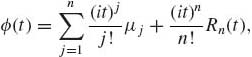
where |Rn(t)| ≤ 3E{|X|n}, Rn(t) → 0 as t→ 0;
Proof. The proof of (i) and (ii) is based on the fact that |eitx| = 1 for all t and all x. Now, ![]() e−itx dF(x) =
e−itx dF(x) = ![]() (−t) =
(−t) = ![]() . Hence (iii) is proven.
. Hence (iii) is proven.
(iv) Suppose F(x) is symmetric around x0 = 0. Then dF(x) = dF(−x) for all x. Therefore, since sin (−tx) = −sin (tx) for all x, ![]() sin (tx) dF(x) = 0, and
sin (tx) dF(x) = 0, and ![]() (t) is real. If
(t) is real. If ![]() (t) is real,
(t) is real, ![]() (t) =
(t) = ![]() . Hence
. Hence ![]() X(t) =
X(t) = ![]() −X(t). Thus, by the one–to–one correspondence between
−X(t). Thus, by the one–to–one correspondence between ![]() and F, for any Borel set B, P{ X
and F, for any Borel set B, P{ X ![]() B} = P{−X
B} = P{−X ![]() B} = P{X
B} = P{X ![]() −B}. This implies that F is symmetric about the origin.
−B}. This implies that F is symmetric about the origin.
(v) If E{|X|n} <∞, then E{|X|r} < ∞ for all 1 ≤ r ≤ n. Consider
![]()
Since ![]() ≤ |x|, and E{|X|}<∞, we obtain from the Dominated Convergence Theorem that
≤ |x|, and E{|X|}<∞, we obtain from the Dominated Convergence Theorem that
Hence μ1 = ![]()
![]() (1)(0).
(1)(0).
Equations (1.8.28)–(1.8.29) follow by induction. Taylor expansion of eiy yields
![]()
where |θ1| ≤ 1 and |θ2| ≤ 1. Hence
where
![]()
Since |cos (ty)| ≤ 1, |sin (ty)| ≤ 1, evidently Rn(t) ≤ 3E{|X|n}. Also, by dominated convergence, ![]() , Rn(t) = 0.
, Rn(t) = 0.
(vi) By induction on n. Suppose ![]() (2)(0) exists. By L’Hospital’s rule,
(2)(0) exists. By L’Hospital’s rule,
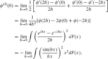
By Fatou’s Lemma,
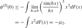
Thus, μ2 ≤ − ![]() (2) (0) < ∞. Assume that 0 < μ2k < ∞. Then, by (v),
(2) (0) < ∞. Assume that 0 < μ2k < ∞. Then, by (v),
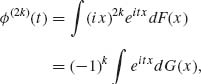
where dG(x) = x2kdF(x), or
![]()
Notice that G(∞) = μ2k < ∞. Thus, ![]() is the characteristic function of the distribution G(x)/G(∞). Since
is the characteristic function of the distribution G(x)/G(∞). Since ![]() > 0,
> 0, ![]() x2h + 2 dF(x) =
x2h + 2 dF(x) = ![]() x2 dG(x) < ∞. This proves that μ2k < ∞ for all k = 1, …, n.
x2 dG(x) < ∞. This proves that μ2k < ∞ for all k = 1, …, n.
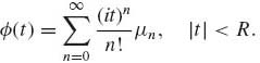
(vii) Assuming (1.8.31), if 0 < t0 < R, ![]() . Therefore,
. Therefore,
![]()
By Stirling’s approximation, ![]() (n!)1/n = 1. Thus, for 0 < t0 < R,
(n!)1/n = 1. Thus, for 0 < t0 < R,
![]()
Accordingly, by Cauchy’s test, ![]() < ∞. By (iv), for any n ≥ 1, for any t, |t| ≤ t0
< ∞. By (iv), for any n ≥ 1, for any t, |t| ≤ t0
![]()
where |![]() (t)| ≤ 3
(t)| ≤ 3![]() E{|X|n}. Thus, for every t,
E{|X|n}. Thus, for every t, ![]() , which implies that
, which implies that
![]() QED
QED
1.9 MODES OF CONVERGENCE
In this section we formulate many definitions and results in terms of random vectors X = (X1, X2, ···, Xk)’, 1 ≤ k < ∞. The notation ||X|| is used for the Euclidean norm, i.e., ||x||2 = ![]() .
.
We discuss here four modes of convergence of sequences of random vectors to a random vector.
A sequence Xn is said to converge in distribution to X, Xn ![]() X if the corresponding distribution functions Fn and F satisfy
X if the corresponding distribution functions Fn and F satisfy
(1.9.1) ![]()
for every continuous bounded function g on ![]() k.
k.
One can show that this definition is equivalent to the following statement.
A sequence {Xn} converges in distribution to X, Xn ![]() X if
X if ![]() Fn(x) = F(x) at all continuity points x of F.
Fn(x) = F(x) at all continuity points x of F.
If Xn ![]() X we say that Fn converges to F weakly. The notation is Fn
X we say that Fn converges to F weakly. The notation is Fn ![]() F or Fn
F or Fn ![]() F.
F.
We define now convergence in probability.
A sequence {Xn} converges in probability to X, Xn ![]() X if, for each
X if, for each ![]() > 0,
> 0,
(1.9.2) ![]()
We define now convergence in rth mean.
A sequence of random vectors {Xn} converges in rth mean, r > 0, to X, Xn ![]() X if E{||Xn − X||r} → 0 as n→ ∞.
X if E{||Xn − X||r} → 0 as n→ ∞.
A fourth mode of convergence is
A sequence of random vectors {Xn} converges almost–surely to X, Xn ![]() X, as n→ ∞ if
X, as n→ ∞ if
(1.9.3) ![]()
The following is an equivalent definition.
Xn ![]() X as n → ∞ if and only if, for any
X as n → ∞ if and only if, for any ![]() > 0,
> 0,
Equation (1.9.4) is equivalent to
![]()
But,
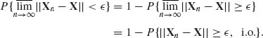
By the Borel–Cantelli Lemma (Theorem 1.4.1), a sufficient condition for Xn ![]() X is
X is
(1.9.5) 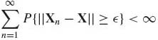
for all ![]() > 0.
> 0.
Theorem 1.9.1. Let {Xn} be a sequence of random vectors. Then
Proof. (a) Since Xn ![]() X, for any
X, for any ![]() > 0,
> 0,
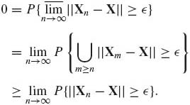
The inequality (1.9.6) implies that Xn ![]() X.
X.
(b) It can be immediately shown that, for any ![]() > 0,
> 0,
![]()
Thus, Xn ![]() X implies Xn
X implies Xn ![]() X.
X.
(c) Let ![]() > 0. If Xn ≤ x0 then either X ≤ x0 +
> 0. If Xn ≤ x0 then either X ≤ x0 + ![]() 1, where 1 = (1, …, 1)’, or ||Xn − X|| >
1, where 1 = (1, …, 1)’, or ||Xn − X|| > ![]() . Thus, for all n,
. Thus, for all n,
![]()
Similarly,
![]()
Finally, since Xn ![]() X,
X,
![]()
Thus, if x0 is a continuity point of F, by letting ![]() → 0, we obtain
→ 0, we obtain
![]() QED
QED
Theorem 1.9.2 Let {Xn} be a sequence of random vectors. Then
For proof, see Ferguson (1996, p. 9). Part (b) is implied also from Theorem 1.13.3.
Theorem 1.9.3 Let {Xn} be a sequence of nonnegative random variables such that Xn ![]() X and E{Xn} → E{X}, E{X} < ∞. Then
X and E{Xn} → E{X}, E{X} < ∞. Then
Proof. Since E{Xn} → E{X}<∞, for sufficiently large n, E{Xn} < ∞. For such n,
![]()
But,
![]()
Therefore, by the Lebesgue Dominated Convergence Theorem,
![]()
This implies (1.9.7). QED
1.10 WEAK CONVERGENCE
The following theorem plays a major role in weak convergence.
Theorem 1.10.1. The following conditions are equivalent.
For proof, see Ferguson (1996, pp. 14–16).
Theorem 1.10.2. Let {Xn} be a sequence of random vectors in ![]() k, and Xn
k, and Xn ![]() X. Then
X. Then
![]()
Proof. (i) Let g: ![]() l →
l → ![]() be bounded and continuous. Let h(x) = g(f(x)). If x is a continuity point of f, then x is a continuity point of h, i.e., C f
be bounded and continuous. Let h(x) = g(f(x)). If x is a continuity point of f, then x is a continuity point of h, i.e., C f ![]() C(h). Hence P{X
C(h). Hence P{X ![]() C(h)} = 1. By Theorem 1.10.1 (c), it is sufficient to show that E{g(f(Xn))} → E{g(f(X))}. Theorem 1.10.1 (d) implies, since P{X
C(h)} = 1. By Theorem 1.10.1 (c), it is sufficient to show that E{g(f(Xn))} → E{g(f(X))}. Theorem 1.10.1 (d) implies, since P{X ![]() C(h)} = 1 and Xn
C(h)} = 1 and Xn ![]() X, that E{h(Xn)} → E{h(X)}.
X, that E{h(Xn)} → E{h(X)}.
(ii) According to Theorem 1.10.1 (b), let g be a continuous function on ![]() k vanishing outside a compact set. Thus g is uniformly continuous and bounded. Let
k vanishing outside a compact set. Thus g is uniformly continuous and bounded. Let ![]() > 0, find δ > 0 such that, if ||x − y|| < δ then |g(x) − g(y)| <
> 0, find δ > 0 such that, if ||x − y|| < δ then |g(x) − g(y)| < ![]() . Also, g is bounded, say |g(x)| ≤ B < ∞. Thus,
. Also, g is bounded, say |g(x)| ≤ B < ∞. Thus,
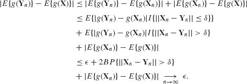
Hence Yn ![]() X.
X.
(iii)
![]()
Hence, from part (ii), ![]() . QED
. QED
As a special case of the above theorem we get
Theorem 1.10.3 (Slutsky’s Theorem) Let {Xn} and {Yn} be sequences of random variables, Xn![]() X and Yn
X and Yn ![]() c. Then
c. Then
(1.10.1) 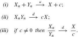
A sequence of distribution functions may not converge to a distribution function. For example, let Xn be random variables with
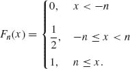
Then, ![]() Fn(x) =
Fn(x) = ![]() for all x. F(x) =
for all x. F(x) = ![]() for all x is not a distribution function. In this example, half of the probability mass escapes to −∞ and half the mass escapes to +∞. In order to avoid such situations, we require from collections (families) of probability distributions to be tight.
for all x is not a distribution function. In this example, half of the probability mass escapes to −∞ and half the mass escapes to +∞. In order to avoid such situations, we require from collections (families) of probability distributions to be tight.
Let ![]() = {Fu, u
= {Fu, u ![]()
![]() } be a family of distribution functions on
} be a family of distribution functions on ![]() k.
k. ![]() is tight if, for any
is tight if, for any ![]() > 0, there exists a compact set C
> 0, there exists a compact set C ![]()
![]() k such that
k such that
![]()
In the above, the sequence Fn(x) is not tight.
If ![]() is tight, then every sequence of distributions of
is tight, then every sequence of distributions of ![]() contains a subsequence converging weakly to a distribution function. (see Shiryayev, 1984, p. 315).
contains a subsequence converging weakly to a distribution function. (see Shiryayev, 1984, p. 315).
Theorem 1.10.4. Let {Fn} be a tight family of distribution functions on ![]() . A necessary and sufficient condition for Fn
. A necessary and sufficient condition for Fn ![]() F is that, for each t
F is that, for each t ![]()
![]() ,
, ![]()
![]() n(t) exists, where
n(t) exists, where ![]() n(t) =
n(t) = ![]() eitx dFn(x) is the characteristic function corresponding to Fn.
eitx dFn(x) is the characteristic function corresponding to Fn.
For proof, see Shiryayev (1984, p. 321).
Theorem 1.10.5 (Continuity Theorem) Let {Fn} be a sequence of distribution functions and {![]() n} the corresponding sequence of characteristic functions. Let F be a distribution function, with characteristic function
n} the corresponding sequence of characteristic functions. Let F be a distribution function, with characteristic function ![]() . Then Fn
. Then Fn ![]() F if and only if
F if and only if ![]() n (t)→
n (t)→ ![]() (t) for all t
(t) for all t ![]()
![]() k. (Shiryayev, 1984, p. 322).
k. (Shiryayev, 1984, p. 322).
1.11 LAWS OF LARGE NUMBERS
1.11.1 The Weak Law of Large Numbers (WLLN)
Let X1, X2, … be a sequence of identically distributed uncorrelated random vectors. Let μ = E{X1} and let ![]() = E{(X1−μ)(X1−μ)’} be finite. Then the means
= E{(X1−μ)(X1−μ)’} be finite. Then the means ![]() n =
n = ![]() converge in probability to μ, i.e.,
converge in probability to μ, i.e.,
(1.11.1) ![]()
The proof is simple. Since cov (Xn, Xn’) = 0 for all n≠ n’, the covariance matrix of ![]() n is
n is ![]()
![]() . Moreover, since E{
. Moreover, since E{![]() n} = μ,
n} = μ,
![]()
Hence ![]() n
n ![]() μ, which implies that
μ, which implies that ![]() n
n ![]() μ. Here tr.{
μ. Here tr.{![]() , } denotes the trace of
, } denotes the trace of ![]() .
.
If X1, X2, … are independent, and identically distributed, with E{X1} = μ, then the characteristic function of ![]() n is
n is
(1.11.2) ![]()
where ![]() (t) is the characteristic function of X1. Fix t. Then for large values of n,
(t) is the characteristic function of X1. Fix t. Then for large values of n,
![]()
Therefore,
(1.11.3) ![]()
![]() (t) = eit’μ is the characteristic function of X, where P{X = μ} = 1. Thus, since eit’μ is continuous at t = 0,
(t) = eit’μ is the characteristic function of X, where P{X = μ} = 1. Thus, since eit’μ is continuous at t = 0, ![]() n
n ![]() μ. This implies that
μ. This implies that ![]() n
n ![]() μ (left as an exercise).
μ (left as an exercise).
1.11.2 The Strong Law of Large Numbers (SLLN)
Strong laws of large numbers, for independent random variables having finite expected values are of the form
![]()
where μi = E{Xi}.
Theorem 1.11.1 (Cantelli) Let {Xn} be a sequence of independent random variables having uniformly bounded fourth–central moments, i.e.,
(1.11.4) ![]()
for all n ≥ 1. Then
(1.11.5) 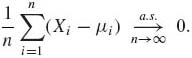
Proof. Without loss of generality, we can assume that μn = E{Xn} = 0 for all n ≥ 1.
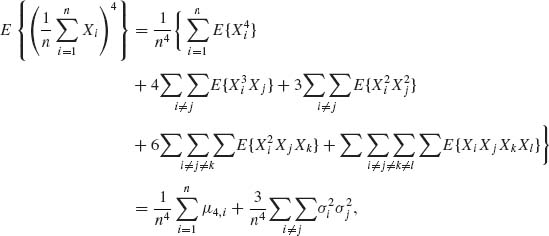
where μ4, i = E{![]() } and
} and ![]() = E{
= E{![]() }. By the Schwarz inequality,
}. By the Schwarz inequality, ![]()
![]() ≤ (μ4, i· μ4j)1/2 for all i≠ j. Hence,
≤ (μ4, i· μ4j)1/2 for all i≠ j. Hence,
![]()
By Chebychev’s inequality,
Hence, for any ![]() > 0,
> 0,
![]()
where C* is some positive finite constant. Finally, by the Borel–Cantelli Lemma (Theorem 1.4.1),
![]()
Thus, P{|![]() n| <
n| < ![]() , i.o.} = 1. QED
, i.o.} = 1. QED
Cantelli’s Theorem is quite stringent, in the sense, that it requires the existence of the fourth moments of the independent random variables. Kolmogorov had relaxed this condition and proved that, if the random variables have finite variances, 0 < ![]() < ∞ and
< ∞ and
(1.11.6) 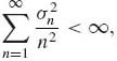
then ![]()
![]() (Xi − μi)
(Xi − μi) ![]() 0 as n→ ∞.
0 as n→ ∞.
If the random variables are independent and identically distributed (i.i.d.), then Kolmogorov showed that E{|X1|} < ∞ is sufficient for the strong law of large numbers. To prove Kolmogorov’s strong law of large numbers one has to develop more theoretical results. We refer the reader to more advanced probability books (see Shiryayev, 1984).
1.12 CENTRAL LIMIT THEOREM
The Central Limit Theorem (CLT) states that, under general valid conditions, the distributions of properly normalized sample means converge weakly to the standard normal distribution.
A continuous random variable Z is said to have a standard normal distribution, and we denote it Z ~ N(0, 1) if its distribution function is absolutely continuous, having a p.d.f.
(1.12.1) ![]()
The c.d.f. of N(0, 1), called the standard normal integral is
(1.12.2) ![]()
The general family of normal distributions is studied in Chapter 2. Here we just mention that if Z ~ N(0, 1), the moments of Z are
(1.12.3) 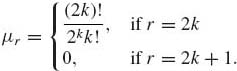
The characteristic function of N(0, 1) is
(1.12.4) 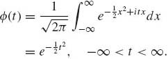
A random vector ![]() = (Z1, …, Zk)’ is said to have a multivariate normal distribution with mean μ = E{Z} = 0 and covariance matrix V (see Chapter 2), Z ~ N(0, V) if the p.d.f. of Z is
= (Z1, …, Zk)’ is said to have a multivariate normal distribution with mean μ = E{Z} = 0 and covariance matrix V (see Chapter 2), Z ~ N(0, V) if the p.d.f. of Z is
![]()
The corresponding characteristic function is
(1.12.5) ![]()
t ![]()
![]() k.
k.
Using the method of characteristic functions, with the continuity theorem we prove the following simple two versions of the CLT. A proof of the Central Limit Theorem, which is not based on the continuity theorem of characteristic functions, can be obtained by the method of Stein (1986) for approximating expected values or probabilities.
Theorem 1.12.1. (CLT) Let {Xn} be a sequence of i.i.d. random variables having a finite positive variance, i.e., μ = E{X1}, V{X1} = σ2, 0 < σ2 < ∞. Then
(1.12.6) ![]()
Proof. Notice that 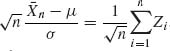 , where
 ![]() , i ≥ 1. Moreover, E{Zi} = 0 and V{Zi} = 1, i ≥ 1. Let
, i ≥ 1. Moreover, E{Zi} = 0 and V{Zi} = 1, i ≥ 1. Let ![]() Z(t) be the characteristic function of Z1. Then, since E{Z} = 0, V{Z} = 1, (1.8.33) implies that
Z(t) be the characteristic function of Z1. Then, since E{Z} = 0, V{Z} = 1, (1.8.33) implies that
![]()
Accordingly, since {Zn} are i.i.d.,
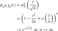
Hence, ![]()
![]() n
n ![]() N(0, 1). QED
N(0, 1). QED
Theorem 1.12.1 can be generalized to random vector. Let ![]() n =
n =  , n ≥ 1. The generalized CLT is the following theorem.
Theorem 1.12.2 Let {Xn} be a sequence of i.i.d. random vectors with E{Xn} = 0, and covariance matrix E{Xn X’n} = V, n ≥ 1, where V is positive definite with finite eigenvalues. Then
(1.12.7) ![]()
Proof. Let ![]() X (t) be the characteristic function of X1. Then, since E{X1} = 0,
X (t) be the characteristic function of X1. Then, since E{X1} = 0,
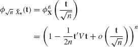
as n→ ∞. Hence
![]() QED
QED
When the random variables are independent but not identically distributed, we need a stronger version of the CLT. The following celebrated CLT is sufficient for most purposes.
Theorem 1.12.3 (Lindeberg–Feller) Consider a triangular array of random variables {Xn, k}, k = 1, …, n, n ≥ 1 such that, for each n ≥ 1, {Xn, k, k = 1, …, n} are independent, with E{Xn, k} = 0 and V{Xn, k} = ![]() . Let Sn =
. Let Sn = ![]() Xn, k and
Xn, k and ![]() =
= ![]()
![]() . Assume that Bn > 0 for each n ≥ 1, and Bn
. Assume that Bn > 0 for each n ≥ 1, and Bn ![]() ∞, as n→ ∞. If, for every
∞, as n→ ∞. If, for every ![]() > 0,
> 0,
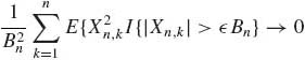
as n→ ∞, then Sn/Bn ![]() N(0, 1) as n → ∞. Conversely, if
N(0, 1) as n → ∞. Conversely, if ![]() as n → ∞ and Sn/Bn
as n → ∞ and Sn/Bn![]() N(0, 1), then (1.12.8) holds.
N(0, 1), then (1.12.8) holds.
For a proof, see Shiryayev (1984, p. 326). The following theorem, known as Lyapunov’s Theorem, is weaker than the Lindeberg–Feller Theorem, but is often sufficient to establish the CLT.
Theorem 1.12.4 (Lyapunov) Let {Xn} be a sequence of independent random variables. Assume that E{Xn} = 0, V{Xn} > 0 and E{|Xn|3}<∞, for all n≥ 1. Moreover, assume that ![]() =
= ![]() V{Xj}
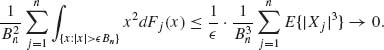
V{Xj} ![]() ∞. Under the condition
∞. Under the condition
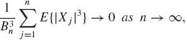
the CLT holds, i.e., Sn/Bn![]() N(0, 1) as n→ ∞.
N(0, 1) as n→ ∞.
Proof. It is sufficient to prove that (1.12.9) implies the Lindberg–Feller condition (1.12.8). Indeed,
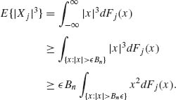
Thus,
 QED
QED
Stein (1986, p. 97) proved, using a novel approximation to expectation, that if X1, X2, … are independent and identically distributed, with EX1 = 0, EX![]() = 1 and γ = E{|X1|3}<∞, then, for all −∞ < x < ∞ and all n = 1, 2, …,
= 1 and γ = E{|X1|3}<∞, then, for all −∞ < x < ∞ and all n = 1, 2, …,
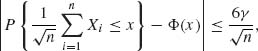
where Φ(x) is the c.d.f. of N(0, 1). This immediately implies the CLT and shows that the convergence is uniform in x.
1.13 MISCELLANEOUS RESULTS
In this section we review additional results.
1.13.1 Law of the Iterated Logarithm
We denote by log2(x) the function log(log(x)), x > e.
Theorem 1.13.1 Let {Xn} be a sequence of i.i.d. random variables, such that E{X1} = 0 and V{X1} = σ2, 0 < σ < ∞. Let Sn = ![]() Xi. Then
Xi. Then
where ![]() (n) = (2σ2n log2(n))1/2, n ≥ 3.
(n) = (2σ2n log2(n))1/2, n ≥ 3.
For proof, in the normal case, see Shiryayev (1984, p. 372).
The theorem means the sequence |Sn| will cross the boundary ![]() (n), n ≥ 3, only a finite number of times, with probability 1, as n → ∞. Notice that although E{Sn} = 0, n ≥ 1, the variance of Sn is V{Sn} = nσ2 and P{|Sn|
(n), n ≥ 3, only a finite number of times, with probability 1, as n → ∞. Notice that although E{Sn} = 0, n ≥ 1, the variance of Sn is V{Sn} = nσ2 and P{|Sn|![]() ∞ } = 1. However, if we consider
∞ } = 1. However, if we consider ![]() then by the SLLN,
then by the SLLN, ![]()
![]() 0. If we divide only by
0. If we divide only by ![]() then, by the CLT,
then, by the CLT, ![]()
![]()
![]() N(0, 1). The law of the iterated logarithm says that, for every
N(0, 1). The law of the iterated logarithm says that, for every ![]() > 0, P
> 0, P ![]() = 0. This means, that the fluctuations of Sn are not too wild. In Example 1.19 we see that if {Xn} are i.i.d. with P{X1 = 1} = P{X1 = −1} =
= 0. This means, that the fluctuations of Sn are not too wild. In Example 1.19 we see that if {Xn} are i.i.d. with P{X1 = 1} = P{X1 = −1} = ![]() , then
, then ![]()
![]() 0 as n→ ∞. But n goes to infinity faster than
0 as n→ ∞. But n goes to infinity faster than ![]() . Thus, by (1.13.1), if we consider the sequence
. Thus, by (1.13.1), if we consider the sequence ![]() then P{|Wn| < 1+
then P{|Wn| < 1+![]() , i.o.} = 1. {Wn} fluctuates between −1 and 1 almost always.
, i.o.} = 1. {Wn} fluctuates between −1 and 1 almost always.
1.13.2 Uniform Integrability
A sequence of random variables {Xn} is uniformly integrable if
(1.13.2) ![]()
Clearly, if |Xn| ≤ Y for all n ≥ 1 and E{Y}<∞, then {Xn} is a uniformly integrable sequence. Indeed, |Xn| I{|Xn| > c} ≤ |Y|I{|Y| > c} for all n ≥ 1. Hence,
![]()
as c → ∞ since E{Y} < ∞.
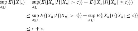
Theorem 1.13.2 Let {Xn} be uniformly integrable. Then,
(1.13.4) ![]()
(1.13.5) ![]()
Proof. (i) For every c > 0
By uniform integrability, for every ![]() > 0, take c sufficiently large so that
> 0, take c sufficiently large so that
![]()
By Fatou’s Lemma (Theorem 1.6.2),
(1.13.7) ![]()
But Xn I{Xn ≥ −c}} ≥ Xn. Therefore,
From (1.13.6)–(1.13.8), we obtain
(1.13.9) ![]()
In a similar way, we show that
(1.13.10) ![]()
Since ![]() is arbitrary we obtain (1.13.3). Part (ii) is obtained from (i) as in the Dominated Convergence Theorem (Theorem 1.6.3). QED
is arbitrary we obtain (1.13.3). Part (ii) is obtained from (i) as in the Dominated Convergence Theorem (Theorem 1.6.3). QED
Theorem 1.13.3. Let Xn ≥ 0, n ≥ 1, and Xn ![]() X, E{Xn} < ∞. Then E{Xn} → E{X} if and only if {Xn} is uniformly integrable.
X, E{Xn} < ∞. Then E{Xn} → E{X} if and only if {Xn} is uniformly integrable.
Proof. The sufficiency follows from part (ii) of the previous theorem.
To prove necessity, let
![]()
Then, for each c ![]() A
A
![]()
The family {XnI{Xn < c} } is uniformly integrable. Hence, by sufficiency,
![]()
for c ![]() A, n → ∞. A has a countable number of jump points. Since E {X}<∞, we can choose c0
A, n → ∞. A has a countable number of jump points. Since E {X}<∞, we can choose c0 ![]() A sufficiently large so that, for a given
A sufficiently large so that, for a given ![]() > 0, E{XI{X≥ c0}} <
> 0, E{XI{X≥ c0}} < ![]() . Choose N0(
. Choose N0(![]() ) sufficiently large so that, for n ≥ N0 (
) sufficiently large so that, for n ≥ N0 (![]() ),
),
![]()
Choose c1 > c0 sufficiently large so that E{XnI{Xn ≥ c1}} ≤ ![]() , n ≤ N0. Then
, n ≤ N0. Then ![]() E{XnI{Xn ≥ c1}} ≤
E{XnI{Xn ≥ c1}} ≤ ![]() . QED
. QED
Lemma 1.13.1 If {Xn} is a sequence of uniformly integrable random variables, then
(1.13.11) ![]()
Proof.
for 0 < c < ∞ sufficiently large. QED
Theorem 1.13.4 A necessary and sufficient condition for a sequence {Xn} to be uniformly integrable is that
and
Proof. (i) Necessity: Condition (1.13.12) was proven in the previous lemma. Furthermore, for any 0 < c <∞,
(1.13.14) 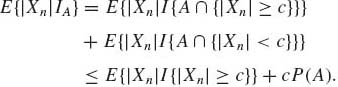
Choose c sufficiently large, so that E{|Xn|I{|Xn|≥ c}} < ![]() and A so that P{A} <
and A so that P{A} < ![]() , then E{|Xn|IA} <
, then E{|Xn|IA} < ![]() . This proves the necessity of (1.13.13).
. This proves the necessity of (1.13.13).
(ii) Sufficiency: Let ![]() > 0 be given. Choose δ (
> 0 be given. Choose δ (![]() ) so that P{A} < δ (
) so that P{A} < δ (![]() ), and
), and ![]() E{|Xn|IA} ≤
E{|Xn|IA} ≤ ![]() .
.
By Chebychev’s inequality, for every c > 0,
![]()
Hence,
The right–hand side of (1.13.15) goes to zero, when c→ ∞. Choose c sufficiently large so that P{|Xn|≥ c} < ![]() . Such a value of c exists, independently of n, due to (1.13.15). Let
. Such a value of c exists, independently of n, due to (1.13.15). Let 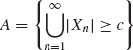 . For sufficiently large c, P{A} <
 ![]() and, therefore,
and, therefore,
![]()
as c→ ∞. This establishes the uniform integrability of {Xn}. QED
Notice that according to Theorem 1.13.3, if E|Xn|r <∞, r ≥ 1 and Xn ![]() X,
X, ![]() E{
E{![]() } = E{Xr} if and only if {Xn} is a uniformly integrable sequence.
} = E{Xr} if and only if {Xn} is a uniformly integrable sequence.
1.13.3 Inequalities
In previous sections we established several inequalities. The Chebychev inequality, the Kolmogorov inequality. In this section we establish some useful additional inequalities.
1. The Schwarz Inequality
Let (X, Y) be random variables with joint distribution function FXY and marginal distribution functions FX and FY, respectively. Then, for every Borel measurable and integrable functions g and h, such that E{g2(X)} < ∞ and E{h2(Y)}<∞,

To prove (1.13.16), consider the random variable Q(t) = (g(X) + th(Y))2, −∞ < t < ∞. Obviously, Q(t) ≥ 0, for all t, −∞ < t < ∞. Moreover,
![]()
for all t. But, E{Q(t)} ≥ 0 for all t if and only if
![]()
This establishes (1.13.16).
2. Jensen’s Inequality
A function g: ![]() →
→ ![]() is called convex if, for any −∞ < x < y < ∞ and 0 ≤ α ≤ 1,
is called convex if, for any −∞ < x < y < ∞ and 0 ≤ α ≤ 1,
![]()
Suppose X is a random variable and E{|X|} < ∞. Then, if g is convex,
To prove (1.13.17), notice that since g is convex, for every x0, −∞ < x0 <∞, g(x) ≥ g(x0) + (x−x0)g* (x0) for all x, −∞ < x <∞, where g* (x0) is finite. Substitute x0 = E{X}. Then
![]()
with probability one. Since E{X−E{X}} = 0, we obtain (1.13.17).
3. Lyapunov’s Inequality
If 0 < s < r and E{|X|r}<∞, then
(1.13.18) ![]()
To establish this inequality, let t = r/s. Notice that g(x) = |x|t is convex, since t > 1. Let ξ = E{|X|s}, and (|X|s)t = |X|r. Thus, by Jensen’s inequality,
![]()
Hence, E{|X|s}1/s ≤ (E{|X|r})1/r. As a result of Lyapunov’s inequality we have the following chain of inequalities among absolute moments.
(1.13.19) ![]()
4. Hölder’s Inequality
Let 1 < p < ∞ and 1 < q <∞, such that ![]() . E{|X|p} < ∞ and E{|Y|q} < ∞. Then
. E{|X|p} < ∞ and E{|Y|q} < ∞. Then
(1.13.20) ![]()
Notice that the Schwarz inequality is a special case of Holder’s inequality for p = q =2.
For proof, see Shiryayev (1984, p. 191).
5. Minkowsky’s Inequality
If E{|X|p} < ∞ and E{|Y|p} < ∞ for some 1 ≤ p <∞, then E{|X + Y|p} < ∞ and
(1.13.21) ![]()
For proof, see Shiryayev (1984, p. 192).
1.13.4 The Delta Method
The delta method is designed to yield large sample approximations to nonlinear functions g of the sample mean ![]() n and its variance. More specifically, let {Xn} be a sequence of i.i.d. random variables. Assume that 0 < V{X} < ∞. By the SLLN,
n and its variance. More specifically, let {Xn} be a sequence of i.i.d. random variables. Assume that 0 < V{X} < ∞. By the SLLN, ![]() n
n ![]() μ, as n→ ∞, where
μ, as n→ ∞, where ![]() n =
n = ![]()
![]() Xj, and by the CLT,
Xj, and by the CLT, ![]() N(0, 1). Let g:
N(0, 1). Let g: ![]() →
→ ![]() having third order continuous derivative. By the Taylor expansion of g(
having third order continuous derivative. By the Taylor expansion of g(![]() n) around μ,
n) around μ,
where Rn = ![]() (
(![]() n−μ)3g(3)(
n−μ)3g(3)(![]() ), where
), where ![]() is a point between
is a point between ![]() n and μ, i.e., |
n and μ, i.e., |![]() n −
n − ![]() | < |
| < |![]() n − μ|. Since we assumed that g(3)(x) is continuous, it is bounded on the closed interval [μ −Δ, μ +Δ]. Moreover, g(3)(
n − μ|. Since we assumed that g(3)(x) is continuous, it is bounded on the closed interval [μ −Δ, μ +Δ]. Moreover, g(3)(![]() )
) ![]() g(3)(μ), as n → ∞. Thus Rn
g(3)(μ), as n → ∞. Thus Rn ![]() 0, as n→ ∞. The distribution of g(μ) + g(1)(μ)(
0, as n→ ∞. The distribution of g(μ) + g(1)(μ)(![]() n − μ) is asymptotically N(g(μ), (g(1)(μ))2σ2/n). (
n − μ) is asymptotically N(g(μ), (g(1)(μ))2σ2/n). (![]() n −μ)2
n −μ)2 ![]() 0, as n→ ∞. Thus,
0, as n→ ∞. Thus, ![]() (g(
(g(![]() n)−g(μ))
n)−g(μ))![]() N(0, σ2(g(1)(μ))2). Thus, if
N(0, σ2(g(1)(μ))2). Thus, if ![]() n satisfies the CLT, an approximation to the expected value of g(
n satisfies the CLT, an approximation to the expected value of g(![]() n) is
n) is
(1.13.23) ![]()
An approximation to the variance of g(![]() n) is
n) is
(1.13.24) ![]()
Furthermore, from (1.13.22)
(1.13.25) ![]()
where
(1.13.26) ![]()
and |![]() −
− ![]() n| ≤ |μ −
n| ≤ |μ − ![]() n| with probability one. Thus, since
n| with probability one. Thus, since ![]() n − μ → 0 a.s., as n→ ∞, and since |g(2) (
n − μ → 0 a.s., as n→ ∞, and since |g(2) (![]() )| is bounded, Dn
)| is bounded, Dn ![]() 0, as n→ ∞, then
0, as n→ ∞, then
(1.13.27) 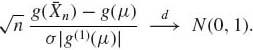
1.13.5 The Symbols op and Op
Let {Xn} and {Yn} be two sequences of random variables, Yn > 0 a.s. for all n ≥ 1. We say that Xn = op(Yn), i.e., Xn is of a smaller order of magnitude than Yn in probability if
(1.13.28) ![]()
We say that Xn = Op(Yn), i.e., Xn has the same order of magnitude in probability as Yn if, for all ![]() > 0, there exists K
> 0, there exists K![]() such that supn P
such that supn P![]() .
.
One can verify the following relations.
(1.13.29) 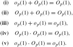
1.13.6 The Empirical Distribution and Sample Quantiles
Let X1, X2, …, Xn be i.i.d. random variables having a distribution F. The function
(1.13.30) 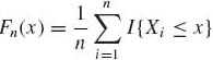
is called the empirical distribution function (EDF).
Notice that E{I{Xi ≤ x}} = F(x). Thus, the SLLN implies that at each x, Fn(x) ![]() F(x) as n → ∞. The question is whether this convergence is uniform in x. The answer is given by
F(x) as n → ∞. The question is whether this convergence is uniform in x. The answer is given by
Theorem 1.13.5 (Glivenko–Cantelli) Let X1, X2, X3, … be i.i.d. random variables. Then
(1.13.31) ![]()
For proof, see Sen and Singer (1993, p. 185).
The pth sample quantile xn, p is defined as
(1.13.32) 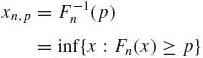
for 0 < p < 1, where Fn(x) is the EDF. When F(x) is continuous then, the points of increase of Fn(x) are the order statistics X(1:n) < ··· < X(n:n) with probability one. Also, Fn(X(i:n)) = ![]() , i = 1, …, n. Thus,
, i = 1, …, n. Thus,
(1.13.33) 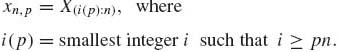
Theorem 1.13.6 Let F be a continuous distribution function, and ξp = F−1(p), and suppose that F(ξp) = p and for any ![]() > 0, F(ξp −
> 0, F(ξp − ![]() ) < p < F(ξp +
) < p < F(ξp + ![]() ). Let X1, …, Xn be i.i.d. random variables from this distribution. Then
). Let X1, …, Xn be i.i.d. random variables from this distribution. Then
![]()
For proof, see Sen and Singer (1993, p. 167).
The following theorem establishes the asymptotic normality of xn, p.
Theorem 1.13.7 Let F(x) be an absolutely continuous distribution, with continuous p.d.f. f(x). Let p, 0 < p < 1, ξp = F−1(p) and f(ξp) > 0. Then
(1.13.34) ![]()
For proof, see Sen and Singer (1993, p. 168).
The results of Theorems 1.13.6–1.13.7 will be used in Chapter 7 to establish the asymptotic relative efficiency of the sample median, relative to the sample mean.