
9
Impact of Battery Energy Storage Systems and Demand Response Program on Locational Marginal Prices in Distribution System
Saikrishna Varikunta* and Ashwani Kumar
Department of Electrical Engineering, National Institute of Technology, Kurukshetra, Haryana, India
Abstract
The pricing of electricity consumption is an important aspect of power system economics. Electricity pricing based on the Locational Marginal Price (LMP) is gaining attention in electricity markets all around the world due to the better distribution system markets and energy-efficient distribution of electricity with hybrid combination of energy resources. The pricing should be such that the generation, transmission, and end users should all benefit. The fairness of pricing should be present in the pricing scheme. By using Locational Marginal Price (LMP), active and reactive power pricings can be made. With LMP-based pricing, the generator, transmission operator and end users are fairly benefited. It is also believed that with the knowledge of the LMPs end users can manage their load and try to participate in a Demand Response (DR) program.
In this chapter, the Locational Marginal Price (LMP) of active and reactive powers is obtained considering the role of storage devices and the impact of a demand response program on their variations. The impact of installation of Shunt capacitor, Energy Storage System (ESS) like Battery Energy Storage System (BESS) and Load participation in Demand Response (DR) program on the LMPs is discussed. Based on the LMPs, the technical and economic aspects are studied. The OPF problem has been solved using General Algebraic Modeling System (GAMS) software and the results are plotted using MATLAB.
Keywords: Battery energy storage systems, demand response program, locational marginal prices, microgrids
9.1 Introduction
Today’s power system network is very complex and there is a paradigm shift in its operation from conventional to automatic due to the amalgamation of renewable energy sources with conventional power plants. The operation of the power sector is now competitive with wholesale selling and buying of the power in a pool and bilateral mode. The power is being sold at a competitive price in the electricity markets. The transparent pricing mechanisms are gaining importance for fair and transparent operation of the power sector where locational marginal prices are essential to computing prices of the electricity. Locational Marginal Pricing (LMPs) represents the cost of buying and selling power at different locations within wholesale electricity markets, usually called Independent System Operators (ISOs). LMPs give information about the three components, Energy Price, Congestion Cost, and Losses [1]. The LMPs give fair information of cost components and information about the network operation and behavior of load. Many authors have done research in this area of obtaining the cost. Both real and reactive power pricing is essential to establish what consumers pay for their usage of electricity.
With the emergence of smart grid, many new components are being added to the network like battery energy storage systems and renewable energy sources, and demand-side management is also playing a key role in the operation of the system. A brief overview of the battery energy storage systems and demand-side management follows.
9.1.1 Battery Energy Storage System (BESS)
Energy storage is a bridge between intermittent sources and fluctuating loads. The energy produced at one moment can be used later by storing it. One type of energy storage is electricity storage. Mechanical, electrochemical (or batteries), thermal, electrical, and hydrogen storage methods are some of the major technologies that fall under the umbrella of energy storage technologies.
A Battery Energy Storage System (BESS) is a type of energy storage system (ESS) that collects energy from various sources, and stores it in batteries (rechargeable type) for subsequent utilization. Different BESS-Battery types are Li-Ion batteries, Lead-Acid (PbA) batteries, Nickel-Cadmium (Ni-Cd) batteries, Sodium sulfur (Na-S) batteries and Flow batteries, etc.
Different components in the Battery Energy Storage System (BESS) are the Energy management system (EMS), the Battery system, and Power Conversion System (PCS). The battery system includes the battery pack, battery management system (BMS), and battery thermal management system (B-TMS). The cells are protected by BMS and the cell temperature is controlled by B-TMS. EMS will ensure the safety and reliability of the system overall operation. PCS will monitor and control various power electronic components which are used in the power conversion (Bi-directional) between the grid and the battery.
Energy storage device applications vary depending on the time needed to connect to the generator, transmitter, and place of use of energy, and on energy use.
Some of the BESS applications in Grid-Utility are given below with different size ranges [12]:
- Electric energy time-shift [1-500 MW]:
Electric energy time-shifting is acquiring affordable electric energy during periods when prices or system marginal costs are low in order to charge the storage system and consume or sell the stored energy at a later time when prices or costs are high.
- Electric Supply Capacity [1-500 MW]:
Energy storage may be used to postpone or lessen the requirement to purchase capacity in the wholesale electricity market, based on the situation in a particular electric supply system.
- Regulation [10-40 MW]:
Among the auxiliary services, regulation is one of those for which storage is particularly well suited.
- Spinning, non-spinning, and supplemental reserves [10-100MW]:
When a portion of the usual sources of electric supply is suddenly unavailable, an electric grid must have reserve capacity that may be used. BESS will act as reserve capacity,
- Voltage Support [1-10MVAr]:
Reactive power control can be carried out in addition to active power management by a battery energy storage system (BESS) outfitted with an appropriately sophisticated inverter (Power Conversion Systems). This enables the deployment of a battery energy storage system in a grid to additionally assist the grid with reactive power and adjust the power factor of loads.
- Black Start [5-50 MW]:
Black start refers to the power system’s capacity to rebound from a blackout by restarting selected components. In order to create an interconnected system once more, disconnected power plants must be started separately and progressively rejoined. When a blackout occurs and the grid needs to be reset from scratch, then BESS is will provide start-up to the power plants such that they can be brought back on-line.
- Load following [1-100 MW]:
A BESS that is the appropriate fit may also offer longer-duration services, such as load-following and ramping services, to make sure supply keeps up with demand. To make sure supply and demand are balanced, a properly scaled BESS may also offer longer-duration services like load-following and ramping services.
- Demand Charge Management [50 KW-10 MW]:
End users can employ energy storage systems to lower their total expenses for energy consumption by lowering their demand during peak hours which are set by the utility. BESS will be able to compensate for the reduced demand during peak hours; thereby the load burden on the grid utility decreases and so not only the end users but also the utility grid will benefit.
- Others applications and benefits are: Transmission and Distribution (T&D) upgrade deferral, Transmission congestion management, power quality, etc.
9.1.2 Demand Response Program
The demand of different consumers may change its patterns as per the operating conditions in a system that may respond to changes in the price of electricity during a whole day. Such demand may have the incentive to reduce their demand during the peak loads and may help the reduction and valley shaving during the peak hours of load demand. This will help to have payments that may be designed to lower electricity use at times of high wholesale market prices. The demand response has the capability of changing the electric usage by the customers/end users from their normal consumption patterns as per the response to changes in the price of electricity during the whole day or in real time and can have the mechanisms for incentive payments that are designed to lower electricity usage during the time of high wholesale market prices or when system security and reliability is threatened [13]. The Demand response programs are classified into two categories: Dispatchable (or) Incentive-based programs and Non-Dispatchable (or) Time-Based programs. Some of the Incentive-Based demand response programs are Direct control, Interruptible/Curtailable, Demand binding, Emergency market, capacity market, ancillary services market type programs, etc. Some of the Time-Based demand response programs are Time-of-Use, Critical Peak Pricing, Extreme Day CPP, Extreme Day pricing, and Real-Time pricing programs, etc.
Some of the Benefits of DR program are:
- The bill savings and incentive payments received by consumers who alter their power usage in response to time-varying electricity tariffs or incentive-based programs are referred to as participant financial benefits.
- The load shape can be altered.
- The customer has control over their consumption, and Easy to implement.
- With the DR program the reduction of outages in the system is observed, thereby reliability benefits such as operational safety and sufficiency savings can be achieved.
- At distribution level the benefits of DR program implementation are: shifting and reducing the peak demand, meeting future energy needs, postponement of distribution system capital investment, voltage-related issues are resolved, reduction of congestion at the substation and making integration of renewable energy resources simple, etc.
- At the transmission level, the benefits of DR program are reduction of transmission congestion, postponement of transmission expansion projects and improvement of transmission network reliability, etc.
- At the generation level the benefits due to DR are lower generating equipment’s operational costs, etc.
Therefore, it is essential to find the impact of storage devices and the role of demand-side management on the LMPs. Reference [2], discussed the important role of LMPs in restructured wholesale power markets. The work reported by the authors extensively presented and analysed various AC and DC optimal power flow models to better understand the calculation of LMPs. In [3], the authors proposed active and reactive power pricing on the basis of marginal costs. In [4] the real-time reactive power pricing is discussed by considering the price depended on demand function; the author took minimization of active power generation cost as the objective function. In [5], the authors included the reactive power production cost along with the active power production cost in objective function; the Optimal Power Flow (OPF) problem is solved using the sequential quadratic programming (SQP) method, and various factors affecting the reactive power LMPs are discussed. In [6] the optimal reactive power management is discussed and the OPF objective function is to minimize the cost of reactive power and it is solved by using Particle Swarm Optimization (PSO) algorithm. In [7] a new approach for reactive power pricing and the cost allocation of reactive power is proposed and a quadratic cost function for reactive power support is calibrated. In [8] the authors used a modified OPF with the objective function of minimizing both the real and reactive power from which LMPs of real and reactive power has been obtained; they also discussed the significance of negative LMPs and showed some finding regarding the nature of LMP during Off-peak load condition.
The LMPs are obtained by solving the OPF problem by using GAMS programming in [9]. Five different cases are considered in the analysis and for each case the changes in LMPs, their technical and economic aspects are discussed. Based on the LMPs, the Total Revenue generated, Congestion Cost, Revenue of Generator and Profit of Generator are calculated for each case. How the LMPs impacts on economic aspects of generator is also discussed.
The five case studies are: Case 1, the objective function is the minimization of the active power production cost. In Case 2, the reactive power production cost is included in the objective function of case 1. In Case 3, a shunt capacitor is considered and its annual objective function is the modification of case 2 by including the capacitor cost. In Case 4, battery energy storage devices are considered along with shunt capacitor, and the objective function consists of the objective function of case 3 including the BESS cost. In Case 5, the LMPs’ applications are studied, like the load is assumed to participate in the Demand Response (DR) program and incentives are provided accordingly for curtailment of load based on the LMPs [10, 11]; the objective function consists of the objective function of case 4 including the utility maximization term. Later in this chapter, due to the installation shunt capacitor, how the reactive power LMPs will change is discussed and due to energy storage devices and load curtailment how the LMPs of active power will change are discussed. An optimization problem has been solved using GAMS programming with CONOPT-NLP solver [15–17].
9.2 Problem Formulation and Solution Using GAMS
The Locational Marginal Price (LMP) is defined as the marginal cost of supplying the next increment of electric energy at a certain location while taking into account the generation marginal cost and the physical features of the transmission system [14]. The LMPs of Active and Reactive power are obtained by solving the OPF problem, in which the objective function is minimized subject to equality and inequality constraints. In this chapter, the OPF problem in solved using GAMS programming with CONOPT-NLP solver [15–17]. In this section the various objective functions for different cases and constraints are mentioned.
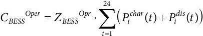
The OPF in this chapter is formulated for five case studies. In case 1, the objective function is minimization of the active power production cost and it is given by equation (9.1). In case 2, the objective function is to minimize both active and reactive power production cost, without a shunt capacitor in the system and it is given by the equation (9.4). In case 3, the objective function of case 2 is modified by adding the Capacitor investment cost to it; here a variable shunt capacitor is placed at bus 4 in the system. In case 4, the modification in the system is an Energy Storage Device which is added along with the Shunt Capacitor at bus 4; here objective function for this case is obtained by modifying objective function of Case 3 by adding the BESS investment cost (per day) and the operation cost, In case 5, the load at bus 2 is assumed to be participated in DR program and the load that bus is curtailed and incentives are paid accordingly, and the objective function is obtained by modifying case 4 by adding utility maximization function, for this case is the modification of case 4.
9.2.1 Objective Functions for Case Studies: Case 1 to Case 5
9.2.1.1 Case 1: Is Minimization of the Active Power Production Cost
The Objective function of the OPF is represented as

Where( C)1 is the sum of cost of real power production cost of all generator. Cpi Pgi is the cost of production of active power by the ith generator. G is total no. of generators in the system.
The active power production cost can be represented as
9.2.1.2 Case 2: Minimization of the Active Power Production and Reactive Power Production Cost
The active power production cost is represented in $/hr. The reactive power production cost is often neglected. The reactive production cost is also known as Opportunity cost. During heavy loading conditions the generator will supply the reactive power to the system by reducing some of its active power generation [5]. So, thereby the cost of active power selling due to reactive power production is reduced. The opportunity cost of the generator depends on the real-time dispatch and the price of active power at that instant. Hence, the exact calculation of cost of reactive power production is complex. For simplicity, the cost of reactive power production of ith generator, Cqi (Qgi) is represented as [18]:

Where Sgi,max is the nominal apparent power of the generator and k is the profit rate of active power produced, usually its range is [5% – 10%]. Here, it is assumed that Sgi,max = Pgi,max.
The Objective function for Case 2 is represented as:

9.2.1.3 Case 3: Minimization of the Active Power Production and Reactive Power Production Cost Along with Capacitor Placement
In this case, a shunt capacitor is placed in the system to provide reactive power support and to improve the voltage profile. The cost function/model of the capacitor investment cost of the jth capacitor is given by the equation (9.5):

Where C is the total number of shunt capacitors present in the system. Here, the investment cost is considered as $11600/MVAr, the operating period (or) the life span of capacitor is assumed to be 15 years (15 yrs = 15*8760 hrs = 131400 hrs), the usage rate (u) is taken as 2/3, the above Equation can be simplified as:
Here, Qcj in MVAr’s. The Objective function of this case is obtained by modifying case 2 objective function, and it is given by:
 (9.7)
(9.7)9.2.1.4 Case 4: Minimization of the Active Power Production and Reactive Power Production Cost Including Capacitor and BESS Cost
In this case, Energy Storage System (ESS) like Battery Energy Storage System (BESS) is considered in a distribution system along with the shunt capacitor.
The State of Charge (SOC) equation of simple ESS/BESS model is given by:
Where ![]() and
and ![]() are Charging and Discharging power of ESS/ BESS at time t, ηchar and ηdis are charging and discharging efficiency rates, i is the bus no. and Δt is the time interval length.
are Charging and Discharging power of ESS/ BESS at time t, ηchar and ηdis are charging and discharging efficiency rates, i is the bus no. and Δt is the time interval length.
The BESS Size is optimally obtained solving the problem using GAMS taking the cost equations in the optimization problem and the cost equations are given (9.9, 9.10) and are refereed in [19, 20]:
The Annual investment cost of BESS:
Where

![]() and
and ![]() are investment cost of the BESS Capacity and Power respectively.
are investment cost of the BESS Capacity and Power respectively. ![]() and
and ![]() are the rated BESS Capacity and Power respectively.
are the rated BESS Capacity and Power respectively.
ABESS is the coefficient to calculate BESS annual cost. rin and y are interest rate and life time of BESS respectively. The Operational cost of BESS:
where ![]() is the operational cost of the BESS.
is the operational cost of the BESS.
The Objective function of case 4 is given by:
9.2.1.5 Case 5: Minimization of the Active Power Production and Reactive Power Production Cost Including Capacitor and BESS Cost and Taking the Impact of Demand Response Program
In this case, the load at any particular bus is assumed to participate in the Demand Response (DR) Program. For curtailed active power demand, the incentives paid accordingly.
The customer cost function [10] at bus i for load curtailment of xi is
Here i is assumed to be the bus number of the system and N is the number of buses in the system. Also, here it is assumed to be the load is controllable and can be curtailed by the Utility Operator. θi is the willingness of the customer to participate in the DR program and its range is [0 – 1].
K1 and K2 are the customer cost coefficients that are calibrated by the Utility. Here, for simplicity the constants chosen are, K1 = 1/2, K2 = 1 and θ = 0.5.
Let yi be the incentive paid for the curtailment of load xi [11]. The Customer Benefit can be represented as:
The appropriate incentive yi paid for satisfying the customer and utility will be within the range as given below
The term ( yi − λpixi ) in the Equation (9.15) represents the utility maximization function; here in this DR program both the customer and utility are benefited, i.e., the customer will get more or equal amount for this load curtailment based on their customer benefit function, the utility will pay to the customer less than the maximum interruptible value, i.e., it depends on the value of λpixi. Here for this case, the LMPs are taken from the previous case, i.e., without DR program case 4. The budget limit on utility can also be placed to restrict the amount of incentives paid.
The objective function for case 5 is given by:
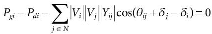
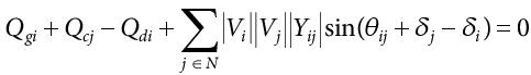
9.2.2 Real and Reactive Power Equality Constraints
The following constraints are considered for the above-mentioned cases:
9.2.2.1 Equality Constraints
The Load Flow Equations are the equality constraints for the OPF problem.
The Active and Reactive power balance equations are (at bus i):
 (9.16)
 (9.17)
The change in equality constraints for different cases are:
For Case 3 to Case 5: Reactive power balance equation
 (9.18)
For Case 4: Real power balance equation
 (9.19)
For Case 5: Real power balance equation

N is the total number of buses in the system.
9.2.2.2 Inequality Constraints: (at any bus i): Voltage, Power Generation, Line Flow, SOC, Battery Energy Storage Power
Voltage Magnitude Constraints
Voltage Angle Constraints
Active Power Generation Constraints
Reactive Power Generation Constraints
Complex (or) Apparent power constraint on generator
Transmission line constraints are limits
Reactive power output constraint of shunt capacitor (This Constraint is included for case 3 and case 4 only)
ESS/BESS constraints:
Charging and Discharging constraints:
SOC limits:
9.2.3 Modified Lagrangian Function
The modified Lagrangian function for the OPF problem (in simplified form) is given by
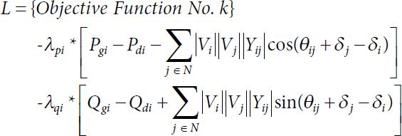
Where k is the Case number. In the above equation (9.31), the Lagrangian function is different for different case. λpi and λqi are the Active and Reactive Power Locational Marginal Prices (LMPs) respectively. The Lagrangian multipliers λpi and λqi are only considered in equation (9.31), the Lagrangian multiplier’s for generation limits, line constraints and voltage limits are not mentioned here even though the conditions are to meet.
9.2.4 Generator Economics Calculations
In this section, we formulate the Total Revenue generated, Congestion Cost, Revenue of Generator and Profit of Generator based on the LMPs [8]. The simple Electricity Market model for the IEEE 5-bus is shown in Figure 9.1, and the power and Money/cash flows can be seen. In Figure 9.1, it can be seen that the power flow starts from generation center to load center; in special cases when renewable energy sources and storage devices included at load center then the power can exchange between load and Transmission system operator (TSO). Here in this chapter as the BESS is added, during discharging period the power from BESS will satisfy the load and it gets paid from TSO. When Load participates in DR program the Load will get paid incentives according to their curtailment by TSO. The revenue is generated from the load is collected by the TSO and TSO will pay to the GENCOs by charging some amount for the congestion if any. The revenue obtained by the GENCOs also includes the cost of the loss.
The total revenue generated by the loads is
 (9.32)
Figure 9.1 Electricity Market Structure for 5-bus system.
The Congestion cost is
 (9.33)
 (9.34)
In, Equation (9.35) the CQ,Congestion is very small value comparted to the CP,Congestion, so an approximation for the Total Congestion Cost is given by
Revenue of Generator is:
Note that here the revenue of generator includes the cost of losses.
Profit of Generator is:
9.3 Case Study: Numerical Computation
A Standard IEEE 5-bus system [21] is considered for the case study and its single line diagram is given in Figure 9.2.
In the IEEE 5-Bus system diagram, for case 3 the shunt capacitor switch is on, for case 4 both the shunt capacitor and BESS switch are closed and for case 5 the load at bus 2 with DR program is used instead of only load. Generator Power Constraints and Cost co-efficient Data are given in Table 9.1. The Line data for the test case is given in Table 9.2.
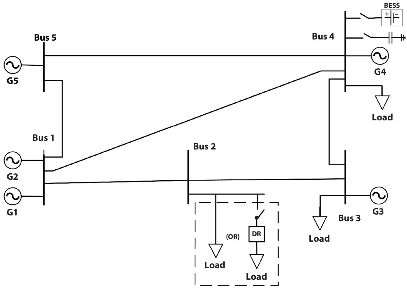
Figure 9.2 Single Line diagram of IEEE 5 bus system.
Table 9.1 Generator power constraints and cost co-efficient data.
| Bus no. | Generator no. | Pmin (MW) | Pmax (MW) | Qmin (MVAr) | Qmax (MVAr) | b ($/MWh) |
|---|---|---|---|---|---|---|
| 1 | 1 | 0 | 40 | -30 | 30 | 14 |
| 1 | 2 | 0 | 170 | -127.5 | 127.5 | 15 |
| 3 | 3 | 0 | 520 | -390 | 390 | 30 |
| 4 | 4 | 0 | 200 | -150 | 150 | 40 |
| 5 | 5 | 0 | 600 | -450 | 450 | 10 |
Table 9.2 Line data.
| From bus | To bus | R (pu) | X (pu) | B/2 (pu) | Limit (MVA) |
|---|---|---|---|---|---|
| 1 | 2 | 0.00281 | 0.0281 | 0.00356 | 400 |
| 1 | 4 | 0.00304 | 0.0304 | 0.00329 | 400 |
| 1 | 5 | 0.00064 | 0.0064 | 0.01563 | 400 |
| 2 | 3 | 0.00108 | 0.0108 | 0.00926 | 400 |
| 3 | 4 | 0.00297 | 0.0297 | 0.00337 | 400 |
| 4 | 5 | 0.00297 | 0.0297 | 0.00337 | 240 |
The Typical(load profile) for the test case is considered as shown in Figure 9.3. The load Pdi + jQdi at each bus i is multiplied with the load factor, which is obtained from the Load profile for time period of 24 hrs. The load during peak hr, i.e., 18th hr at each bus is given in Table 9.3. The ESS/BESS data is given in Table 9.4.

Figure 9.3 Load profile.
Table 9.3 Load at peak hour at each bus.
| Bus no. | Pd (MW) | Qd (Mvar) |
|---|---|---|
| 1 | 0 | 0 |
| 2 | 300 | 98.61 |
| 3 | 300 | 98.61 |
| 4 | 400 | 131.47 |
| 5 | 0 | 0 |
9.4 Results and Discussions
9.4.1 Case 1: Minimization of the Active Power Production Cost
For Case 1, the Demand and Generation of Active and Reactive powers are plotted in Figure 9.4a. The hourly active and reactive power loss and the voltage profile at different bus are plotted in Figure 9.4b and Figure 9.4c, respectively.
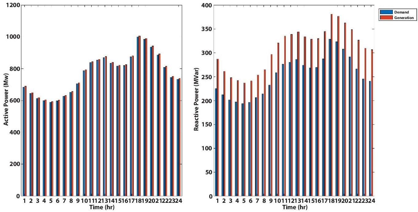
Figure 9.4a Case 1: Active and reactive power demand and generation.

Figure 9.4b Case 1: Active and reactive power loss.

Figure 9.4c Case 1: Voltage profile.
The Active and Reactive Power LMPs at different bus for 24 hrs. period are plotted in Figure 9.4d. Here, the observation is that, LMPs of reactive power at some buses are negative.
The significance of “Negative λq”: It signifies that the load/generator which absorb reactive power at that bus will be paid compensation money and the generator which inject the reactive power at that bus will be penalized.
The Generator Economics calculations are calculated and the results are plotted in Figure 9.4e. In Figure 9.4e it can be seen that at 5th hr. the generator profit is small and negative; also, in the Zoom plot it is shown that the generator revenue is less than the cost of active generation and it is due to the line congestion cost.

Figure 9.4d Case 1: LMPs of active and reactive power at different buses.

Figure 9.4e Case1: Generator economics: Cost and profit.
9.4.2 Case 2: Minimization of the Active Power Production and Reactive Power Production Cost
The Active and Reactive power Demand and Generation graph is shown in Figure 9.5a.
For case 2, the hourly active and reactive power loss and the voltage profile at different bus are plotted in Figure 9.5b and Figure 9.5c, respectively. Compared to the voltage profile of case 1 in Figure 9.4c, the voltage profile obtained in this case is improved.
For Case 2, the Active and Reactive Power LMPs at different bus for 24 hrs period are plotted in Figure 9.5d. Here, the observation is that, LMPs of reactive power at all buses are positive while compared to the LMP’s obtained by case 1 (see in Figure 9.4d). So, in this case there are no negative reactive power LMPs.
For Case 2, Generator Economics calculations are calculated and the results are plotted in Figure 9.5e. In Figure 9.5e, at 5th hr. the generator profit is negative but compared to that in the Figure 9.4e, the value is less negative, i.e., generator incurring loss is less, and also at 5th hr. the cost of generation is greater than the generator revenue.
The important findings by the case 2 results are the LMPs of reactive power at all buses are positive and the voltage profile is slightly improved.

Figure 9.5a Case 2: Active and reactive power demand and generation.

Figure 9.5b Case 2: Active and reactive power loss.

Figure 9.5c Case 2: Voltage profile.

Figure 9.5d Case 2: LMPs of active and reactive power at different buses.

Figure 9.5e Case 2: Generator economics: cost and profit.
9.4.3 Case 3: Minimization of the Active Power Production and Reactive Power Production Cost Along
The Active and Reactive power Demand and Generation and the Capacitor size is shown in Figure 9.6a.
Due to the shunt capacitor placement at bus 4, the voltage profile at bus 4 is further improved. Here, the capacitor is considered to be continuously variable over 24 hr.
For Case 3, the hourly active and reactive power loss and the voltage profile at different bus are plotted in Figure 9.6b and Figure 9.6c, respectively. Compared to the voltage profile of case 1 in Figure 9.4c, the voltage profile obtained in this case is improved.

Figure 9.6a Case 3: Active and reactive power demand and generation and capacitor size.

Figure 9.6b Case 3: Active and reactive power loss.

Figure 9.6c Case 3: Voltage profile.
The Capacitor size and its cost at each hour is shown in Figure 9.6d.
For Case 3, the Active and Reactive Power LMPs at different bus for 24 hrs period are plotted in Figure 9.6e. Here, the observation is that, LMPs of reactive power at all buses are positive while compared to the LMPs obtained by case 1 (see in Figure 9.4d). So, in this case there are no negative reactive power LMPs.

Figure 9.6d Case 3: Capacitor size and cost vs. time.

Figure 9.6e Case 3: LMPs of active and reactive power at different buses.
For Case 3, Generator Economics calculations are calculated and the results are plotted in Figure 9.6f. In Figure 9.6f, at 5th hr the generator profit is negative but compared to that in the Figure 9.4e, the value is less negative, i.e., generator incurring loss is less, and also at 5th hr the cost of power generation is greater than the generator revenue. The important findings by the case 3 results are the LMPs of reactive power at all buses are positive, the reactive power production cost is reduced, active and reactive power losses are reduced and voltage profile is improved.

Figure 9.6f Case 3: Generator economics: cost and profit.
9.4.4 Case 4: Minimization of the Active Power Production and Reactive Power Production Cost
In this case, a ESS/BESS is added along with the shunt capacitor at bus 4, and the objective function of this case is mentioned in Section 9.2. The ratings of ESS/BESS are given in Table 9.4. The Active and Reactive power Demand and Generation and the Capacitor size is shown in Figure 9.7a.
Due to the ESS/BESS installation the change in active power LMPs is observed. The shunt capacitor will make change in the reactive power LMPs; also the voltage profile at bus 4 is improved.
For case 4, the hourly active and reactive power loss and the voltage profile at different bus are plotted in Figure 9.7b and Figure 9.7c respectively. Compared to the voltage profile of case 1 in Figure 9.4c, the voltage profile obtained in this case is improved.
The ESS/BESS SOC curve and its Discharging and Charging power over a 24hr period is shown in Figure 9.7d. The Capacitor size and its cost at each hour is shown in Figure 9.7e.
For Case 4, the Active and Reactive Power LMP’s at different bus for 24 hrs. period are plotted in Figure 9.7f. Here, the observation is that, LMPs of active power at peak load, i.e., at 18th hr. there is change in LMPs compared to the case 3 LMPs. At off peak load i.e., at 5th hr. the active power LMPs are almost equal.
For Case 4, Generator Economics calculations are calculated and the results are plotted in Figure 9.7g. In Figure 9.7g, at 5th hr the generator profit is positive but compared to that of in case 1, 2 and 3, also the noticeable point is that the cost of generation is less than the generator revenue and it can be witnessed in the zoom plot.
Figure 9.7a Case 4: Active and reactive power demand and generation and capacitor size.
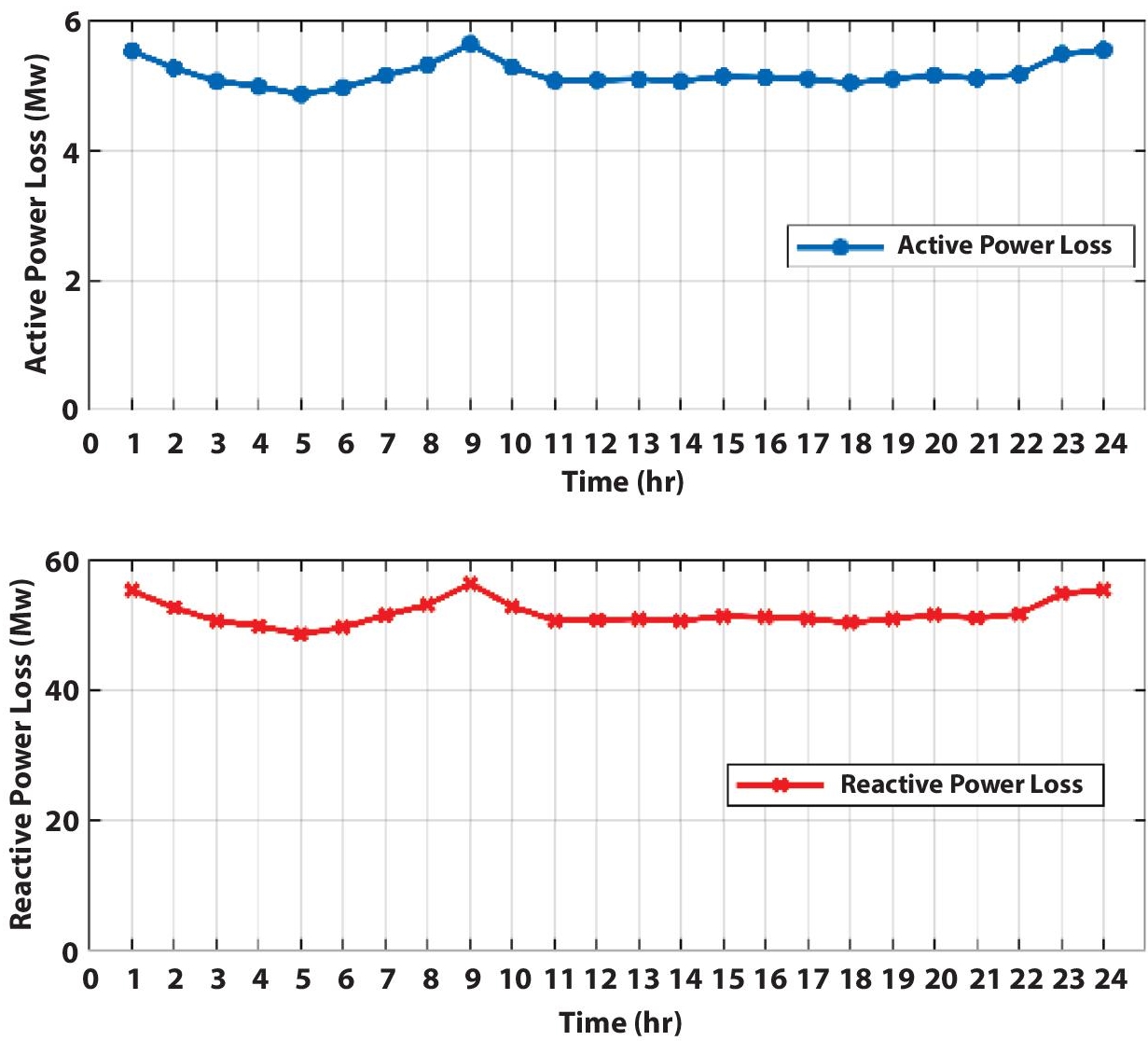
Figure 9.7b Case 4: Active and reactive power loss.

Figure 9.7c Case 4: Voltage profile.

Figure 9.7d Case 4: ESS/BESS: SOC, discharging and charging power.

Figure 9.7e Case 4: Capacitor size and cost vs time.
The important findings of the Case 4 results are that the LMPs of active power undergoes changes due to ESS/BESS installation and the voltage profile is improved by shunt capacitor.

Figure 9.7f Case 4: LMPs of active and reactive power at different buses.

Figure 9.7g Case 4: Generator economics: cost and profit.
9.4.5 Case 5: Minimization of the Active Power Production and Reactive Power Production Cost
This case is an extension to case 4, the objective function and Shunt capacitor and ESS/BESS (installed at bus 4) ratings are the same. In this case, at bus 2 the load is assumed to be participated in Demand Response program and agreed to curtail 50 MW active power load. The Active and Reactive power Demand (Without DR) and Generation and the Capacitor size is shown in Figure 9.8a.
Due to the load participation in DR, the Demand at bus 2 is curtailed optimally and the new total demand is shown in Figure 9.8b and is compared with the demand without DR participation. There is a considerable variations in the demand during peak hours 18 to 21.

Figure 9.8a Case 5: Active and reactive power demand and generation and capacitor size.

Figure 9.8b Case 5: Active power demand: without DR and with DR.
The active power curtailed power at bus 2 and the incentives provided for the curtailment is shown in Figure 9.8c.
From Figure 9.8c, it is seen that at 18th, 19th, 20th hr and 21st hr the active power load curtailed are 21.335 MW. 18.3173 MW, 9.6373 MW and 0.7107 MW, respectively. For the respective load curtailment, the incentives paid are $465.837, $344.68, $97.6967 and $0.86049 respectively. For the incentive payment, the previous case, i.e., case 4 active power LMPs at bus 2 are considered.
For Case 5, the hourly active and reactive power loss and the voltage profile at different bus are plotted in Figure 9.8d and Figure 9.8e, respectively. The ESS/BESS SOC curve and its Discharging and Charging power over 24hr period for case 5 is shown in Figure 9.8f. The Capacitor size and its cost at each hour is shown in Figure 9.8g.
For Case 5, the Active and Reactive Power LMP’s at different bus for 24 hrs. period are plotted in Figure 9.8h.
The LMP comparison of Active power of Case 4 and Case 5 at 18th, 19th, 20th and 21st hr is shown in Figure 9.8i. Due to the DR program the load is curtailed at hr where the peak of demand is observed; the loads which are participating in the DR program will now pay the price less than when they did not participate in the DR program. Here we compare the results of Case 4 and Case 5 active power LMP and a fair reduction in LMP is observed with the respective to the amount of load curtailed For Case 5, Generator Economics calculations are calculated and the results are plotted in Figure 9.8j. In Figure 9.8j, at 5th hr the generator profit is positive, also the cost of generation is less than the generator revenue and it can be witnessed in the zoom plot.
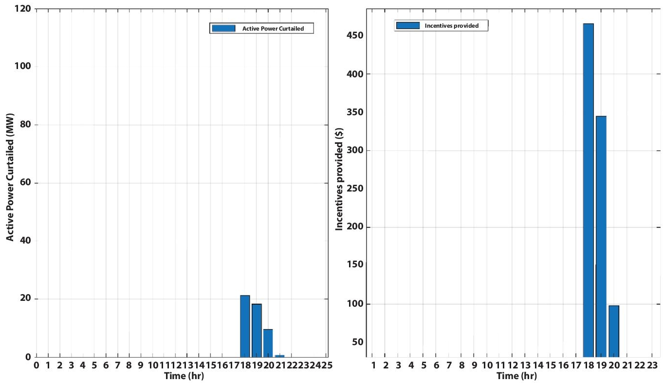
Figure 9.8c Case 5: Load curtailment and incentive payment.

Figure 9.8d Case 5: Active and reactive power loss.
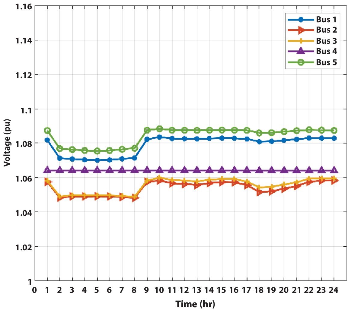
Figure 9.8e Case 5: voltage profile.

Figure 9.8f Case 5: ESS/BESS: SOC, discharging and charging power.

Figure 9.8g Case 5: capacitor size and cost vs. time.

Figure 9.8h Case 5: LMPs of active and reactive power at different buses.
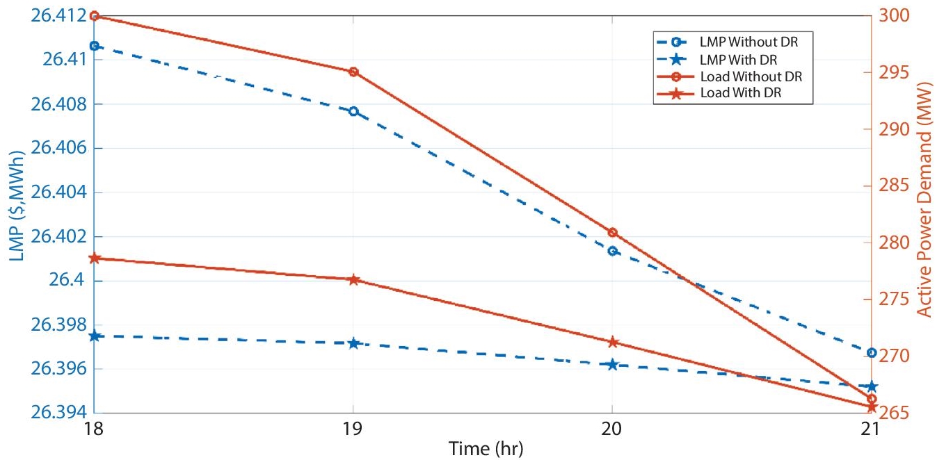
Figure 9.8i Case 5: comparison of active power LMP of case 4 and case 5.
To summarize and compare the results of all 5 cases, for simplicity we only considered the two prominent points, i.e., the two hours i.e., 5th hr (Off-peak) and 18th hr (Peak) to observe the trends of results and the various parameters and are calculated and tabulated in Table 9.5 and Table 9.6 respectively. The active and reactive power LMPs at Off-peak and Peak hours are also tabulated in Table 9.5 and Table 9.6.
From Table 9.5, it is seen that the reactive power production cost is decreased in case 3, case 4 and case 5 while it is compared with the case 2. The active power production cost increases significantly from case 3 to case 5 due to the ESS/BESS installation, i.e., at this off-peak load period the ESS/BESS undergoes charging with zero load reduction. The Active power LMPs from case 1 to case 3 increases (see in Table 9.5) and it’s due to the charging of energy devices; also the reactive power LMPs from case 1 to case 5 decreases as the reactive power support is provided by shunt capacitor. It is also observed that the profit of generator is negative, i.e., generator has to face loss from case 1 to case 3, whereas from case 4 to case 5 the profit is positive and it is appreciated. The reason for the negative profit of generator is the cost of production is greater than the revenue of the generator, and it can be made positive by adding active power support devices like ESS/BESS, Renewable energy sources, etc.

Figure 9.8j Case 5: generator economics: cost and profit.
Table 9.5 Result comparison of all cases at off-peak load.
| Parameter | At off-peak load (at 5th hr) | |||||
|---|---|---|---|---|---|---|
| Case 1 | Case 2 | Case 3 | Case 4 | Case 5 | ||
| Active Power (MW) | Demand | 588.8740 | ||||
| Generation | 593.209 | 593.378 | 593.340 | 642.341 | 653.325 | |
| Loss | 4.335 | 4.504 | 4.466 | 4.860 | 4.987 | |
| Reactive Power (Mvar) | Demand | 193.557 | ||||
| Generation | 236.904 | 238.592 | 138.213 | 142.156 | 147.000 | |
| Loss | 43.347 | 45.035 | 44.656 | 48.599 | 49.874 | |
| Reactive Power Support by Shunt Capacitor (Mvar) | - | - | 100 | 100 | 100 | |
| ESS/BESS | Charging Power (MW) | - | - | - | 48.607 | 48.604 |
| Discharging Power (MW) | - | - | - | 0.000 | 0.000 | |
| Active Power Curtailed (MW) | - | - | - | - | 0 | |
| Incentives paid ($) | - | - | - | - | 0 | |
| Active Power | Bus 1 | 10.042 | 10.051 | 10.048 | 15.000 | 15.000 |
| LMP’s ($/MWh) | Bus 2 | 10.163 | 10.204 | 10.188 | 15.209 | 15.209 |
| Bus 3 | 10.113 | 10.219 | 10.202 | 15.232 | 15.232 | |
| Bus 4 | 10.108 | 10.140 | 10.129 | 15.136 | 15.136 | |
| Bus 5 | 10.000 | 10.000 | 10.000 | 14.934 | 14.934 | |
| Reactive Power LMP’s ($/MVArh) | Bus 1 | 0 | 0.252 | 0.144 | 0.148 | 0.148 |
| Bus 2 | 0.01029 | 0.290 | 0.176 | 0.193 | 0.193 | |
| Bus 3 | 0 | 0.286 | 0.172 | 0.187 | 0.187 | |
| Bus 4 | 0 | 0.268 | 0.140 | 0.141 | 0.141 | |
| Bus 5 | 0 | 0.241 | 0.137 | 0.138 | 0.138 | |
| Active power production cost ($) | 5932.087 | 5933.776 | 5933.396 | 6595.113 | 6759.868 | |
| Reactive power production cost ($) | - | 29.954 | 10.014 | 10.668 | 11.425 | |
| Total power production cost (or) | 5932.087 | 5963.730 | 5943.411 | 6605.781 | 6771.293 | |
| Shunt capacitor return/ cost ($) | - | - | 1324.000 | 1324.000 | 1324.000 | |
| BESS Cost ($ per day) (Operation + Investment) | - | - | - | 2146.614 | 2146.504 | |
| Revenue Generated ($) | 5975.600 | 6050.750 | 6019.113 | 8975.942 | 9258.868 | |
| Congestion Cost ($) | 86.592 | 108.212 | 99.767 | 156.334 | 337.107 | |
| Revenue of Generator ($) | 5889.008 | 5942.538 | 5919.346 | 8819.608 | 8921.760 | |
| Profit of Generator ($) | -43.079 | -21.192 | -20.984 | 2213.828 | 2150.467 | |
Table 9.6 Result comparison for all the cases at peak load.
| Parameter | At peak load (at 18th hr) | ||||||
|---|---|---|---|---|---|---|---|
| Case 1 | Case 2 | Case 3 | Case 4 | Case 5 | |||
| Active Power (MW) | Demand | 1000.000 | |||||
| Generation | 1005.238 | 1004.645 | 1004.510 | 956.431 | 860.710 | ||
| Loss | 5.238 | 4.645 | 4.510 | 5.038 | 5.157 | ||
| Reactive Power (Mvar) | Demand | 328.690 | |||||
| Generation | 381.075 | 375.138 | 281.818 | 309.599 | 312.036 | ||
| Loss | 52.385 | 46.448 | 45.097 | 50.377 | 51.566 | ||
| Reactive Power Support by Shunt Capacitor (Mvar) | - | - | 91.969 | 69.468 | 68.220 | ||
| ESS/BESS | Charging Power (MW) | - | - | - | 0.000 | 0.000 | |
| Discharging Power (MW) | - | - | - | 48.607 | 37.773 | ||
| Active Power Curtail(MW) | - | - | - | - | 21.335 | ||
| Incentives paid ($) | - | - | - | - | 465.837 | ||
| Active Power LMP’s ($/MWh) | Bus 1 | 16.876 | 16.792 | 16.812 | 16.783 | 16.771 | |
| Bus 2 | 26.503 | 26.416 | 26.422 | 26.411 | 26.398 | ||
| Bus 3 | 30.000 | 30.000 | 30.000 | 30.000 | 30.000 | ||
| Bus 4 | 39.684 | 39.862 | 39.781 | 39.730 | 39.644 | ||
| Bus 5 | 10.000 | 10.000 | 10.000 | 10.000 | 10.000 | ||
| Reactive Power LMP’s ($/MVAr) | Bus 1 | 0.347 | 0.658 | 0.556 | 0.598 | 0.602 | |
| Bus 2 | 0.375 | 0.867 | 0.753 | 0.801 | 0.608 | ||
| Bus 3 | 0.122 | 0.680 | 0.560 | 0.571 | 0.584 | ||
| Bus 4 | 0 | 0.306 | 0.132 | 0.132 | 0.132 | ||
| Bus 5 | 0 | 0.276 | 0.180 | 0.217 | 0.216 | ||
| Active power produccost ($) | 17546.740 | 17640.889 | 17653.938 | 15717.607 | 13525.164 | ||
| Reactive power production cost ($) | - | 89.295 | 56.171 | 64.194 | 65.659 | ||
| Total power production cost (or) | 17546.740 | 17730.184 | 17710.108 | 15781.801 | 13590.823 | ||
| Shunt capacitor return/cost ($) | - | - | 1217.672 | 919.754 | 903.235 | ||
| BESS Cost ($ per day) (Operation + Investment) | - | - | - | 2146.614 | 2092.350 | ||
| Revenue Generated ($) | 17901.076 | 33062.380 | 32986.057 | 32949.374 | 32933.084 | ||
| Congestion Cost ($) | 15044.979 | 14922.951 | 14871.921 | 14854.723 | 14844.774 | ||
| Revenue of Generator ($) | 17891.763 | 18139.428 | 18114.136 | 18094.651 | 18088.310 | ||
| Profit of Generator ($) | 354.337 | 409.245 | 404.027 | 2312.850 | 4497.487 | ||
From Table 9.6, the active power generation cost is reduced significantly from Case 3 to Case 5 along with the active power generation, due to the external active power support by ESS/BESS and load reduction through DR program. The reactive power generation cost also decreased from Case 2 to Case 5 as the shunt capacitor provided the reactive power support, thereby the requirement of reactive power generation also decreased. At peak load period, the ESS/BESS will start discharging the power and also the Load undergoes some curtailment as if it is willing to reduce by participation in the DR program, Load are encouraged to participate in DR program mainly at peak load period by providing them incentives.
The active power LMPs at bus 3 and 5 remains constant for all cases; however, at bus 2 and 4 it decreased from case 1 to case 2, and at bus 2 it increased from case 4 to 5. During peak load period, the generator profit is always positive irrespective of case and the profit increases from case 1 to case 5.
9.5 Conclusions
In this chapter, change in Locational Marginal Price (LMP) of active and reactive power are analyzed for different type of objective functions. The impact of installation of Shunt capacitor, Energy Storage System (ESS) like Battery Energy Storage System (BESS) and Load participation in Demand Response (DR) program on the LMPs is discussed. Technical aspects like losses, voltage profile are studied. The various economic factors, like revenue generated, congestion cost, generator revenue, and generator profit are studied. Based on the analysis carried out, the following conclusions are made from the case studies:
- From case 1, the active LMPs are Positive and the LMPs of reactive power are Positive and Negative. By this we can say the LMP can be positive or negative. Negative LMP at a bus means the penalty for injective the power and compensation for drawing power. Here, Losses occur at the generator during off peak load hour.
- From case 2, both active and reactive power LMPs are positive. Here, the voltage profile is improved compared with the case 1 and the losses are also reduced. The generator still faces loss at off-peak load.
- From case 3, due to the shunt capacitor installation the reactive power LMPs at bus 4 is reduced and also the voltage profile is improved. Here, we can say that the reactive power support devices installation will leads to the changes in the reactive power LMPs, i.e., either positive or negative based on the devices which drawing or injecting the reactive power.
- From case 4, due to the BESS installation at bus 4, the active power LMPs changes. Here, the LMPs of this case are compared with LMPs of case 3. During the charging period of BESS, the active power LMP increases because during this period the BESS act like an additional load. During the discharging period of BESS, the active power LMP decreases because during this period the BESS will act like a source. Here in this case during off-peak load condition the generator profit is positive i.e., the revenue of the generator is more than the cost of production.
- From case 5, due to the load at bus 2 participation in DR program the decrease in active power LMP is observed. So, when the load is reduced the LMP also reduced.
So, when there is a change in active and reactive power there will be a change in the active and reactive LMPs. Here, in this chapter, the Shunt capacitor, Battery energy storage system and DR programs are considered, but Renewable energy sources can also be considered and their impact on LMP can also be observed for planning of the hybrid DERs integrated systems by the distribution system operator.
References
- 1. D. Nurse, “What is Locational Marginal Pricing (LMP)?,” 11 Apr. 2018. [Online]. Available: https://www.energyacuity.com/blog/what-is-locational-marginal-pricing-lmp/#:~:text=LMPs%20are%20made%20up%20of,operating%20day%20to%20avoid%20volatility.
- 2. H. Liu, L. Tesfatsion and A. A. Chowdhury, “Locational marginal pricing basics for restructured wholesale power markets,” in 2009 IEEE Power & Energy Society General Meeting, 2009.
- 3. Fred C. Schweppe, Michael C. Caramanis, Richard D. Tabors, Roger E. Bohn, Spot Pricing of Electricity, Springer US, 1988.
- 4. M. L. B. a. S. N. Siddiqi, “Real-time pricing of reactive power: theory and case study results,” in IEEE Transactions on Power Systems,” IEEE Transactions on Power Systems, vol. 6, pp. 23-29, Feb. 1991.
- 5. Y. Dai, Y. X. Ni, F. S. Wen and Z. X. Han, “Analysis of reactive power pricing under deregulation,” in 2000 Power Engineering Society Summer Meeting (Cat. No.00CH37134), 2000.
- 6. B. Mozafari, A. M. Ranjbar, A. R. Shirani and A. Mozafari, “Reactive power management in a deregulated power system with considering voltage stability: Particle Swarm optimisation approach,” in CIRED 2005 - 18th International Conference and Exhibition on Electricity Distribution, 2005.
- 7. S. &. G. R. &. J. H. Hasanpour, “A new approach for cost allocation and reactive power pricing in a deregulated environment,” Electr Eng 91, pp. 27-34, 2009.
- 8. A. Saranya, K. S. Swamp, “Evaluation of locational marginal pricing of electricity under peak and off-peak load conditions,” in 2016 National Power Systems Conference (NPSC), 2016.
- 9. Soroudi A, Power System Optimization Modeling in GAMS, Germany: Springer International Publishing, 2017.
- 10. M. F. a. F. L. Alvarado, “Using utility information to calibrate customer demand management behavior models,” in 2002 IEEE Power Engineering Society Winter Meeting. Conference Proceedings (Cat. No.02CH37309).
- 11. M. Fahrioglu and F. L. Alvarado, “Designing incentive compatible contracts for effective demand management,” IEEE Transactions on Power Systems, vol. 15, pp. 1255-1260, 2000.
- 12. Handbook on Battery Energy Storage System, Philippines: Asian Development Bank, 2018.
- 13. U.S Dept. of Energy, “Benefits of Demand Response in Electricity Markets and Recommendations for Achieving Them: A Report to the United States Congress,” February 2006.
- 14. Yong Fu and Zuyi Li, “Different models and properties on LMP calculations,” in 2006 IEEE Power Engineering Society General Meeting, 2006.
- 15. “GAMS Documentation Center,” 11 November 2021. [Online]. Available: https://www.gams.com/latest/docs/index.html.
- 16. Brooke A., Kendrick D., Meeraus A., GAMS: A User’s Guide, Redwood City: The Scientific Press, 1998.
- 17. E.Rosenthal, Sichard, GAMS-A User’s Guide, Washington, DC, USA: GAMS Development Corporation, 2007.
- 18. Yun Dai and Yixin Ni and C. M. Shen and Fushuan Wen and Z. X. Han and Felix F. Wu, “A study of reactive power marginal price in electricity market,” Electric Power Systems Research, vol. 57, pp. 41-48, 2001.
- 19. L. Zhou, Y. Zhang, X. Lin, C. Li, Z. Cai and P. Yang, “Optimal Sizing of PV and BESS for a Smart Household Considering Different Price Mechanisms,” IEEE Access, vol. 6, pp. 41050-41059, 2018.
- 20. R. G. S. S. a. J. L. M. Moghimi, “Battery energy storage cost and capacity optimization for university research center,” in 2018 IEEE/IAS 54th Industrial and Commercial Power Systems Technical Conference (I&CPS), 2018.
- 21. Fangxing Li and Rui Bo, “Small test systems for power system economic studies,” IEEE PES General Meeting, 2010.
Note
- *Corresponding author: [email protected]