

Fig. 6.33: Illustration of 3-pixel 1-measurement solutions with the minimum l2 norm, l1 norm, and l0 quasi-norm.
Example 10: When the system of imaging equations is under-determined, use 2-pixel (x1, x2) or 3-pixel (x1, x2, x3) examples to illustrate solutions with the minimum l2 norm, l1 norm, and l0 quasi-norm, respectively.
Solution
Let us consider a 2-pixel (x1, x2) case, and there is one measurement. This measurement can be represented as a straight line in the (x1, x2) coordinate system. Any point on the line is a valid solution. The solutions with the minimum l2 norm, l1 norm, and l0 quasi-norm are shown in Figure 6.32, respectively.
In the 3-pixel (x1, x2, x3) case, there can be one measurement or two measurements. If there is one measurement, this measurement can be represented as a plane in the (x1, x2, x3) coordinate system. Any point on the plane is a valid solution. The solutions with the minimum l2 norm, l1 norm, and l0 quasi-norm are shown in Figure 6.33, respectively.

Fig. 6.34: Illustration of 3-pixel 2-measurement solutions with the minimum l2 norm, l1 norm, and l0 quasi-norm.
In the 3-pixel (x1, x2, x3) case, let us consider the case of two measurements. Each measurement can be represented as a plane in the (x1, x2, x3) coordinate system. Two measurements correspond to two planes. These two planes intersect and form a straight line. Any point on the line is a valid solution. The solutions with the minimum l2 norm, l1 norm, and l0 quasi-norm are shown in Figure 6.34, respectively.
6.12Summary
–The main difference between an analytic image reconstruction algorithm and an iterative image reconstruction algorithm is in image modeling. In an analytic algorithm, the image is assumed to be continuous, and each image pixel is a point. The set of discrete pixels is for display purpose. We can make those display points any way we want. However, in an iterative algorithm, a pixel is an area, which is used to form the projections of the current estimate of the image. The pixel model can significantly affect the quality of the reconstructed image.
–Another difference between an analytic image reconstruction algorithm and an iterative image reconstruction algorithm is that the analytic algorithm tries to solve an integral equation, while the iterative algorithm tries to solve a system of linear equations.
–A system of linear equations is easier to solve than an integral equation. This allows the linear equations to model more realistic and more complex imaging geometry and imaging physics. In other words, the iterative algorithm can solve a more realistic imaging problem than an analytic algorithm. As a result, the iterative algorithm usually provides a more accurate reconstruction.
–Iterative algorithms are used to minimize an objective function. This objective function can effectively incorporate the noise in the measurement. Currently, analytic algorithms control noise by frequency windowing.
–The iterative ML-EM and OS-EM algorithms are most popular in emission tomography image reconstruction. They assume Poisson noise statistics. The transmission data counterparts exist.
–Even though noise is modeled in the objective function, the reconstructed image is still noisy. There are five methods to control noise.
–The first method is to stop the iterative algorithm early, before it converges. This simple method has a drawback that it may result in an image with nonuniform resolution. One remedy is to iterate till convergence and apply a post low-pass filter to suppress the noise.
–The second method is to replace the flat, nonoverlapping pixels by smooth, overlapping pixels to represent the image. The method can remove the artificially introduced high frequency components by the flat, non-overlapping pixels in the image. A drawback of using smooth, overlapping pixels is the increased computational complexity. One remedy is to use the traditional flat, nonoverlapping pixels and apply a low-pass filter to backprojected images.
–The third method is to model more accurate imaging geometry and physics in the projector/backprojector pair. The aim of this method is to reduce the deterministic discrepancy between the projection model and the measured data.
–The fourth method is to use the correct noise model to set up an objective function. The author’s personal belief is that the noise model that is based on the joint probability density function is not very critical. You can have a not-so-accurate noise model (i.e., a not-so-accurate joint probability density function), but you must have the accurate variance. The important part is to incorporate a correct measurement noise variance to weigh the data. It is not as important to worry about whether the noise is strictly Gaussian, strictly Poisson, and so on.
–The fifth method is the use of prior knowledge. If the projection data do not carry enough information about the object, due partially to insufficient measurements and partially to noise, prior knowledge about the object can supplement more information about the object and make the iterative algorithm more stable. Be careful that if the prior knowledge is not really true, it can mislead the algorithm to converge to a wrong image.
–The readers are expected to understand how the system of imaging equations is set up and how the iterative ML-EM algorithm works in this chapter.
Problems
![]()
| Problem 6.1 | Some iterative algorithms, for example, the ART and OS-EM algorithms, update the image very frequently. For those algorithms, the processing order of the data subsets is important. In this problem, we use the ART algorithm to graphically solve a system of linear equations {L1, L2, L3, L4} with two variables as shown in the figure below. The initial estimated solution is X0. Solve the system with two different orders: (a) L1 → L2 → L3 → L4 and (b) L1 → L3 → L2 → L4, respectively. Compare their performance in terms of convergence rate.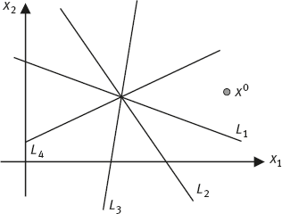 |
| Problem 6.2 | The iterative ML-EM algorithm or the iterative OS-EM algorithm, has many modified versions. One of the versions introduces a new parameter h: This parameter h usually takes a real value in the interval between 1 and 5. The purpose of using this parameter h is to increase the iteration step size and make the algorithm converge faster. If the parameter h is chosen in the interval between 0 and 1, it reduces the iteration step size. Does this new algorithm satisfy the property of total count conservation as studied in Worked Problem 8 in this chapter? If that property is not satisfied any more, you can always scale the newly updated image with a factor. Find this scaling factor so that the total count is conserved for each iteration. |
| Problem 6.3 | The modified algorithm discussed in Problem 6.2 can only be used in emission imaging applications, because the linear equations are weighted by Poisson variance of the emission measurements. One can develop a similar algorithm for the transmission measurements to find the attenuation map of the object as  where the measurements are modeled as Ni = N0e– ∑j aij,j. Here, we do not take the logarithm and convert these non-linear equations into linear equations. Instead, we go ahead and solve this system of nonlinear equations Ni = N0e– ∑j aij,j directly. Use the Taylor expansion to convert this algorithm to its corresponding additive updating form. Discuss how the parameter h controls the iteration step size, how the nonlinear equations are weighted, and what the weighting quantity is. |
| Problem 6.4 | We have learned that in an iterative image reconstruction algorithm the projector should model the imaging system as accurately as possible. For a set of practical data acquired from an actual imaging system, there is a simple way to verify whether the modeling in the projector is accurate enough. This method is described as follows. Run an iterative algorithm to reconstruct the image. After the algorithm is converged, calculate and display the data discrepancy images at every view. A discrepancy image is the difference between the projection of the reconstructed image and the measured projection data, or is the ratio of the projection of the reconstructed image to the measured projection data. If the projector models the imaging system accurately, you do not see the shadow of the object in the discrepancy images and you only see the random noise in the discrepancy images. Verify this method with a computer simulation. |
| Problem 6.5 | In Example 7, a bad Bayesian constraint β(x1 – x2)2 in eq. (6.124) was chosen. Redo Example 7 with a different Bayesian constraint of your choice. For example, you could choose a minimum norm constraint. |
Bibliography
[1]Bai C, Zeng GL, Gullberg GT, DiFilippo F, Miller S (1998) Slab-by-slab blurring model for geometric point response and attenuation correction using iterative reconstruction algorithms. IEEE Trans Nucl Sci 45:2168–2173.
[2]Barrett HH, Wilson DW, Tsui BMW (1994) Noise properties of the EM algorithm, I. Theory. Phys Med Biol 39:833–846.
[3]Beekman F, Kamphuis C, Viergever M (1996) Improved SPECT quantitation using fully three-dimensional iterative spatially variable scatter response compensation. IEEE Trans Med Imaging 15:491–499.
[4]Byrne CL (1996) block-iterative methods for image reconstruction from projections. IEEE Trans Imaging Process 5:792–794.
[5]Candès E, Romberg J, Tao T (2006) Robust uncertainty principles: Exact signal reconstruction from highly incomplete frequency information. IEEE Trans Inf Theory 52:489–509.
[6]Censor Y, Eggermont PPB, Fordon D (1983) Strong underrelaxation in Kaczmarz’s method for inconsistent system. Numer Math 41:83–92.
[7]Chang L (1979) Attenuation and incomplete projection in SPECT. IEEE Trans Nucl Sci 26:2780–2789.
[8]Chen GH, Tang J, Hsieh YL (2009) Temporal resolution improvement using PICCS in MDCT cardiac imaging. Med Phys 36:2130–2135.
[9]Chiao PC, Rogers WL, Fessler JA, Clinthorne NH, Hero AO (1994) Model-based estimation with boundary side information or boundary regularization. IEEE Trans Med Imaging 13:227–234.
[10]Dempster AP, Laird NM, Rubin DB (1977) Maximum likelihood from incomplete data via the EM algorithm. J Royal Stat Soc B 39: 1–38.
[11]DiBella E, Barclay A, Eisner R, Schaefer R (1996) A comparison of rotation-based methods for iterative reconstruction algorithms. IEEE Trans Nucl Sci 43:3370–3376.
[12]Donoho D (2006) Compressed sensing. IEEE Trans Inf Theory 52:1289–1306.
[13]Elbakri A, Fessler JA (2002) Statistical image reconstruction for polyenergetic x-ray computed tomography. IEEE Trans. Med. Imag., 21:89–99.
[14]Fessler J (1996) Mean and variance of implicitly defined biased estimators (such as penalized maximum likelihood): Applications to tomography. IEEE Trans Image Processing 5:493–506.
[15]Fessler J, Hero A (1994) Space-alternating generalized expectation maximization algorithm. IEEE Trans Signal Process 42:2664–2677.
[16]Fessler JA, Rogers WL (1996) Spatial resolution properties of penalized-likelihood image reconstruction: Space-invariant tomography. IEEE Trans Imaging Process 5: 1346–1358.
[17]Frey EC, Ju ZW, Tsui BMW (1993) A fast projector-backprojector pair for modeling the asymmetric spatially-varying scatter response in SPECT imaging. IEEE Trans Nucl Sci 40:1192–1197.
[18]Geman S, Geman D (1984) Stochastic relaxation, Gibbs distributions, and Bayesian restoration of images. IEEE Trans Pattern Anal Mach Intell 6:721–741.
[19]Gilbert P (1972) Iterative methods for the reconstruction of three dimensional objects from their projections. J Theor Biol 36:105–117.
[20]Gindi G, Lee M, Rangarajan A, Zubal IG (1991) Bayesian reconstruction of functional images using registered anatomical images as priors. In: Colchester ACF, Hawkes DJ (eds) Information Processing in Medical Imaging, Springer-Verlag, New York, 121–131.
[21]Gordon R, Bender R, Herman GT (1970) Algebraic reconstruction techniques (ART) for three-dimensional electron microscopy and X-ray photography. J Theor Biol 29: 471–481.
[22]Hebert TJ, Leahy R (1992) Statistic-based MAP image reconstruction from Poisson data using Gibbs priors. IEEE Trans Signal Process 40:2290–2303.
[23]Herman GT (1980) Image Reconstruction from Projections: The Fundamentals of Computerized Tomography, Academic Press, New York.
[24]Hsieh YL, Zeng GL, Gullberg GT (1998) Projection space image reconstruction using strip functions to calculate pixels more “natural” for modeling the geometric response of the SPECT collimator. IEEE Trans Med Imaging 17: 24–44.
[25]Hudson HM, Larkin RS (1994) Accelerated image reconstruction using ordered subsets of projection data. IEEE Trans Med Imaging 13:601–609.
[26]Hwang DS, Zeng GL (2005) A new simple iterative reconstruction algorithm for SPECT transmission measurement. Med Phys 32:2312–2319.
[27]Hwang DS, Zeng GL (2005) Reduction of noise amplification in SPECT using smaller detector bin size. IEEE Trans Nucl Sci 52:1417–1427.
[28]Hwang DS, Zeng GL (2006) Convergence study of an accelerated ML-EM algorithm using bigger step size. Phys Med Biol 51:237–252.
[29]Qi J (2003) A unified noise analysis for iterative image estimation. Phys Med Biol 48:3505–3519.
[30]Kacmarz S (1937) Angenaherte Aufosung von Systemen linearer Gleichungen. Bull Acad Polon Sci A 35:355–357.
[31]King, Miller TR (1985) Use of a nonstationary temporal Wiener filter in nuclear medicine. Eur J Nucl Med 10:458–461.
[32]Lalush DS, Tsui BMW (1993) A generalized Gibbs prior for maximum a posteriori reconstruction in SPECT. Phys Med Biol 38:729–741.
[33]Lalush DS, Tsui BMW (1994) Improving the convergence of iterative filtered backprojection algorithms. Med Phys 21:1283–1286.
[34]Lange K (1990) Convergence of EM image reconstruction algorithms with Gibbs smoothing. IEEE Trans Med Imaging 9:439–446.
[35]Lange K, Carson R (1984) EM reconstruction algorithms for emission and transmission tomography. J Comput Assist Tomogr 8:306–316.
[36]Leng S, Tang J, Zambelli J, Nett B, Tolakanahalli, R, Chen GH (2008) High temporal resolution and streak-free four-dimensional cone-beam computed tomography. Phys Med Biol 53:5653–5673.
[37]Lewitt R (1992) Alternatives to voxels for image representation in iterative reconstruction algorithms. Phys Med Biol 37:705–716.
[38]Lewitt RM, Muehllehner G (1986) Accelerated iterative reconstruction for positron emission tomography based on the EM algorithm for maximum likelihood estimation. IEEE Trans Med Imaging 5:16–22.
[39]Liang Z (1993) Compensation for attenuation, scatter, and detector response in SPECT reconstruction via iterative FBP methods. Med Phys 20:1097–1106.
[40]Liang Z, Jazczak R, Greer K (1989) On Bayesian image reconstruction from projections: uniform and nonuniform a priori source information. IEEE Trans Med Imaging 8:227–235.
[41]Liow J, Strother SC (1993) The convergence of object dependent resolution in maximum likelihood based tomographic image reconstruction. Phys Med Biol 38:55–70.
[42]Lucy LB (1974) An iterative technique for the rectification of observed distribution. Astrophys J 79:745–754.
[43]Naraynan VM, King MA, Soare E, Byrne C, Pretorius H, Wernick MN (1999) Application of the Karhunen-Loeve transform to 4D reconstruction of gated cardiac SPECT images. IEEE Trans Nucl Sci 46:1001–1008.
[44]Nuyts J, Michel C, Dupont P (2001) Maximum-likelihood expectation-maximization reconstruction of sinograms with arbitrary noise distribution using NEC-transformations. IEEE Trans Med Imaging 20:365–375.
[45]Pan TS, Yagle AE (1991) Numerical study of multigrid implementations of some iterative image reconstruction algorithms. IEEE Trans Med Imaging 10:572–588.
[46]Pan X, Wong WH, Chen CT, Jun L (1993) Correction for photon attenuation in SPECT: Analytical framework, average attenuation factors, and a new hybrid approach. Phys. Med. Biol. 38: 1219–1234.
[47]Panin VY, Zeng GL, Gullberg GT (1999) Total variation regulated EM algorithm. IEEE Trans Nucl Sci 46,:2202–2210.
[48]Qi J, Leahy RM (1999) Fast computation of the covariance of MAP reconstructions of PET images. Proc SPIE 3661:344–355.
[49]Rucgardson WH (1972) Bayesian-based iterative method of image restoration. J Opt Soc Am A 62:55–59.
[50]Shepp LA, Vardi Y (1982) Maximum likelihood estimation for emission tomography. IEEE Trans Med Imaging 1:113–121.
[51]Snyder DL, Miller MI (1985) The use of sieves of stabilize images produced with the EM algorithm for emission tomography. IEEE Trans Nucl Sci 32:3864–3872.
[52]Tanaka E (1987) A fast reconstruction algorithm for stationary positron emission tomography based on a modified EM algorithm. IEEE Trans Med Imaging 6:98–105.
[53]Trzasko J, Manduca A (2009) Highly undersampled magnetic resonance image reconstruction via homotopic l0-minimization. IEEE Trans Med Imaging 28:106–121.
[54]Wallis JW, Miller TR (1993) Rapidly converging iterative reconstruction algorithms in single-photon emission computed tomography. J Nucl Med 34:1793–1800.
[55]Wilson DW, Tsui BMW, Barrett HH (1994) Noise properties of the EM algorithm, II. Monte Carlo Simulations. Phys Med Biol 39:847–871.
[56]Yu H, Wang G (2009) Compressed sensing based interior tomography. Phys Med Biol 54:2791–2805.
[57]Zeng GL, Gullberg GT (2000) Unmatched projector/backprojector pairs in an iterative reconstruction algorithm. IEEE Trans Med Imaging 19:548–555.
[58]Zeng GL, Hsieh YL, Gullberg GT (1994) A rotating and warping projector-backprojector for fan-beam and cone-beam iterative algorithm. IEEE Trans Nucl Sci 41:2807–2811.
[59]Zeng GL, Gullberg, Tsui BMW, Terry JA (1991) Three-dimensional iterative reconstruction algorithms with attenuation and geometric point response correction. IEEE Trans Nucl Sci 38:693–702.
[60]Zhang B, Zeng GL (2006) An immediate after-backprojection filtering method with blob-shaped window functions for voxel-based iterative reconstruction. Phys Med Biol 51:5825–5842.