7MRI reconstruction

The magnetic resonance imaging (MRI) physics is quite different from that of transmission or emission imaging as we discussed in the previous chapters. This chapter first introduces the imaging physics of MRI, showing how the MRI signals are formed. We will see that the MRI signals are in the Fourier domain and the image reconstruction is achieved via the inverse Fourier transform.

7.1The “M”

The MRI working principle is quite different from that of emission and transmission tomography. MRI is an image of “proton density” in a cross section of the patient. The data in MRI can be simplified as weighted plane integrals of the proton density function in that plane with “frequency”-dependent weighting functions.

In this chapter, we present a watered-down version of the MRI principle. The goal of regular MRI is to get a picture of the distribution of hydrogen atoms (H+) within the patient body.

The hydrogen atom is simply a proton that carries a positive charge and is continuously spinning. A spinning charge generates a magnetic field around it, as if it were a tiny magnet (see Figure 7.1). We call this tiny magnet a “magnetic moment,” $\stackrel{\rightharpoonup }{\mu }$, which is a vector. The orientation is important for a vector.

In the absence of a strong external magnetic field, the proton magnetic moments are randomly oriented inside the body. Thus, the net magnetic moment is zero $\stackrel{\rightharpoonup }{0}$ (see Figure 7.2).

When a strong external magnetic field is applied, the net magnetic moment is no longer zero. We denote this net magnetic moment as a vector $\stackrel{\rightharpoonup }{\text{M}}$ (see Figure 7.3.) must point out that even in this case, not all are pointing in the same direction. About half of them point in the direction of the magnetic field, and the other half point in the opposite direction. Therefore, the magnitude of is very small and is proportional to

$\frac{\gamma \hslash B_o}{2KT},$

where T is the absolute temperature of the patient (in K), K is the Boltzmann constant (8.62 – 10-11 MeV/K), h is the Planck constant (6.6252 10–27 ergs), B0 is the magnetic strength (in Tesla), and γ is an atom-dependent constant (42.58 MHz/Tesla for H+) called the gyromagnetic ratio. We can see that a stronger magnetic field helps generate a stronger signal.

Fig. 7.1: A spinning proton acts like a tiny magnet.

Fig. 7.2: The net magnetic moment is zero without a strong external magnetic field.

Fig. 7.3: In the strong external magnetic field a small nonzero net magnetization can be observed.

Another concept that we need to explain MRI physics is precession. Let us take a look at a spinning toy top (or a gyroscope). Besides spinning, there is another motion: the spin axis rotates around the direction of gravity (an external force). This motion of the spin axis rotating about the direction of gravity is referred to as precession (see Figure 7.4). If the top does not spin, precession won’t happen; it just falls.

We must point out that it is not accurate to use classic physics to explain MRI physics. A more accurate explanation should use quantum mechanics. A neutron with no net electric charge can also act like a tiny magnet and has a magnetic moment. Therefore, besides the hydrogen atoms, MRI can also, in principle, image a nucleus with either an odd atomic number or an odd mass number, for example, 13C, 14N, 19F, 23Na, and 31P. On the other hand, MRI cannot image atomic nuclei consisting of an even number of protons and even number of neutrons, because they do not have unpaired protons or neutrons. Paired protons or neutrons have zero magnetic moment.

Fig. 7.4: A spinning toy top precesses about a vertical axis due to the gravity.

7.2The “R”

We have a vector , called net magnetic moment, which is spinning by itself. Normally, the vector points at the same direction of the external magnetic field 0. If we somehow knock the vector off balance, and is not in the direction of 0 anymore, then the vector will precess about the direction of 0 just as the toy top precesses about the direction of gravity (see Figure 7.5). The precession frequency is called the Larmor frequency and is given as

${\omega }_0=\gamma B_0,$

where B0 is the external magnetic field strength, and is the gyromagnetic ratio. For aproton, γ = 42.58 MHz/Tesla. If the MRI machine has a magnetic field of 1.5 Tesla, then the Larmor frequency is approximately 64 MHz, which is close to the frequency range of an FM radio.

The MRI signal is nothing but this 64 MHz radio frequency (RF) electromagnetic wave sent out from the patient body after the net magnetic moment is somehow knocked off balance. Thus, the MRI signal is also called the RF signal. The strength of the signal is proportional to the proton density inside the patient.

Fig. 7.5: Protons precess at the Larmor frequency ω0.

To knock the net magnetic moment off balance is not an easy task. In order to move the vector , we need to create a virtual situation so that the vector does not feel the existence of the external 0 field.

We will first put the vector on a virtual rotating merry-go-round or a rotating platform (see Figure 7.6), which is rotating at the Larmor frequency. We will later find a way to create precession while the vector is on that rotating platform. The vector now is currently standing on the rotating platform upright and is spinning on its own axis; there is no motion relative to the platform. Even if the vector is not standing upright and it has a nonzero angle with the vertical line, vector will stay with that angle and will not have any motion relative to the platform.

Next, we step on the rotating platform and apply a new magnetic field 1, orthogonal to the main magnetic field 0. On the rotating platform, the vector does not feel the existence of the main field 0; it only feels the push from the new field 1. Since is not aligned with 1, it will precess about the direction of 1 (see Figure 7.7) at a precession frequency ω1 = γB1. Once reaches the platform floor, we turn the new field 1 off. Thus, the mission of knocking off is accomplished. The 1 field is only turned on very briefly; it is called a 90° RF pulse if it is turned off as soon as touches the platform floor.

Fig. 7.6: The magnetization vector does not precess relative to the rotating platform.

Fig. 7.7: On the rotating platform, the effect of the main field can be ignored. Only the new B1 field is effective.

What is this 1 field anyway? The magnetic field 1 is applied on a virtual rotating platform, which rotates at the Larmor frequency, say 64 MHz for a proton in a 1.5 Tesla MRI machine. Therefore, 1 is an alternating electromagnetic RF field with the same frequency as the Larmor frequency. Another term for the same frequency is the resonance frequency. The 1 RF signal is sent to the patient through an RF coil, which is basically an antenna. The procedure of turning the 1 RF field on and knocking off balance is called RF excitation.

After RF excitation, we turn off 1. Now the net magnetic moment is not in the equilibrium state, but in the excited state. The vector is precessing about the main field direction 0, and RF signals that contain the patient proton density information are emitted. The excited state is unstable. After excitation, the vector then goes through the relaxation period and eventually returns to the original equilibrium state, where the vector points to the 0 direction (see Figure 7.8). In a Cartesian system, the 0 direction is the z direction, and the “platform floor” is the x–y plane.

Fig. 7.8: Relaxation of the magnetization vector.

The x and y components of the vector make up the MRI signal. After relaxes back to its equilibrium position, both its x and y components are zero; hence, no more signals can be detected. Another RF pulse excitation is needed for further data acquisition. This procedure is repeated over and over again until enough data are acquired for imaging.

7.3The “I”

The RF signal emitted by the patient as described in Section 7.2 cannot be used to form an image because it is a combined signal from everywhere. We need a way to code the location information. This is achieved by the gradient coils.

In the MRI machine, there are many coils. The main large superconducting coil immersed in liquid helium is used to generate the strong static 0 field. There are RF coils, which are used to emit RF pulses for excitation and to receive RF imaging signals. There are other coils in the machine to create gradients; they are x-gradient coils, y-gradient coils, and z-gradient coils.

7.3.1To obtain z-information: slice selection

The z-gradient coils are shown in Figure 7.9. The currents in the two coils are running in the opposite directions and generate the local magnetic fields to enhance and reduce the main field 0, respectively. The resultant magnetic field is still pointing in the z direction; however, the field strength is stronger at locations with larger z values and is weaker at locations with smaller z values. These coils create a gradient of the magnetic field strength in the z direction.

Fig. 7.9: The z-gradient coils create a non-uniform field in the z-direction.

This z-gradient makes a nonuniform magnetic field, which results in different Larmor frequencies ω for a different z position. The Larmor frequency is ω0 only at one z-slice. We turn on and offthe z-gradient and the 1 RF pulse at the same time. The 1 RF pulse is at the frequency of ω0. According to the resonance frequency principle, only one z-slice of the patient body is affected by the RF pulse. That is, only the protons in this particular z-slice get excited and send out the RF signal (see Figure 7.10).

Fig. 7.10: Slice selection is done by the z-gradient and the B1 field.

7.3.2To obtain x-information: frequency encoding

We use the x-gradient to provide the x-position information. When we are ready to receive the RF signal from the patient, we turn on the x-gradient. The x-gradient is generated by the x-gradient coils, and it makes the strength of the main magnetic field vary in the x-direction. The principle of using x-gradient to code x-position is illustrated in Figure 7.11. Using the relation ω = γB, stronger magnetic field B gives the higher frequency. Thus, the x-location can be determined by the received frequency.

The x-gradient coils are depicted in Figure 7.12. We assume that the x- direction is the direction from the patient’s right ear to left ear. The x-gradient is turned on only when the RF signal is received, and this gradient is also called the readout gradient. Do not turn it on during slice selection. When you turn two gradients on at the same time, they will combine and form a gradient in the third direction.

7.3.3To obtain y-information: phase encoding

After slice selection and before RF signal readout, we turn on the y-gradient for a short time. Before a gradient is turned on, at all locations precess at the same frequency (i.e., same speed). However, when the y-gradient is turned on, the field strength at a different y-position is different. As a result, at a different y-position precesses at a different Larmor frequency (e.g., precession at a faster rate for a position with a larger y value, Figure 7.13). After the y-gradient is on for a short while, it is turned off. At this moment, at a different y-position will arrive at a different phase (i.e., angle). This phase carries the information of the y-position.

Fig. 7.11: Stronger field produces higher frequency.

Fig. 7.12: The x-gradient coils generate a nonuniform magnetic field in the readout direction.

Fig. 7.13: The y-gradient causes the phase displacement as a function of y-location.

The y-gradient coils look exactly like the x-gradient coils, except for a 90°rotation. The effective gradient is confined to the gap between two pairs of the coils(see Figure 7.14).

The time diagram shown in Figure 7.15 summarizes this basic MRI data acquisition procedure. This procedure is repeated many times. At each time, a different value of the y-gradient is used. The next section will show that the acquired data is nothing but the 2D Fourier transform of the image f(x, y), which is closely related to the proton density distribution inside the patient body. A 2D inverse Fourier transform is used to reconstruct the image. A typical MRI image is shown in Figure 7.16. There is a small negative pulse in front of the x-gradient readout pulse. The purpose of it is to create an “echo” to make the strongest signal at the center.

Fig. 7.14: The y-gradient coils make the magnetic field non-uniform in the y direction.

Fig. 7.15: The timing diagram for an MRI pulse sequence.

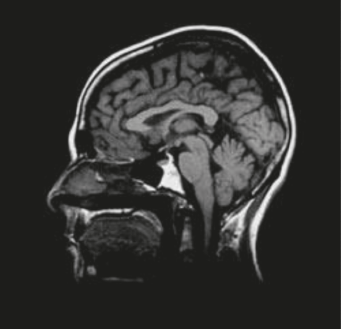
Fig. 7.16: An MRI of the head.

7.4Mathematical expressions

In this section, we assume that a slice selection has been done and (x, y) is a function of x and y. The vector (x, y) can be decomposed into the x-component Mx(x, y), the y-component My(x, y), and the z-component Mz(x, y). We define a complex function f(x, y) as

$f(x,y)=M_x(x,y)+i{M}_y(x,y).$

The goal of MRI is to obtain this function f(x, y) and display its magnitude f(x, y) as the final output for the radiologists to read.

Let us first consider the effect of the readout (x) gradient. When the x-gradient is turned on, the magnetic field strength is a function of x as

$B(x)=B_0+x{G}_x$

and the associated Larmor frequency is calculated as

$\omega (x)=\gamma (B_0+x{G}_x).$

At readout, the function f(x, y) will be encoded as

$f(x,y)\cos (2\pi \omega (x)t)=f(x,y)\cos (2\pi \gamma (B_0+x{G}_x)t),$

where γB0 is the carrier frequency and has no contribution for image reconstruction. In the MRI receiver there is a demodulator that can remove this carrier frequency. After the removal of the carrier frequency, the leftover baseband signal is given as

$f(x,y)\cos (2\pi \gamma x{G}_{x}t).$

Since the signal comes from the entire x-y plane, the received baseband signal is the summation of the signals from each location (x, y):

${\displaystyle \underset{-\infty }{\overset{\infty }{\int }}{\displaystyle \underset{\infty }{\overset{\infty }{\int }}f(x,y)}}\cos (2\pi \gamma x{G}_{x}t)dxdy.$

Second, let us consider the effect of the phase-encoding (y)-gradient. When the y-gradient is turned on for a period of time T, the magnetic field strength is a function of y as

$B(y)=B_0+y{G}_y$

and the associated Larmor frequency is calculated as

$\omega \left(y\right)=\gamma \left(B_0+y{G}_y\right).$

After the period of T, the phase change is a function of y as

$\varphi \left(y\right)=T\omega \left(y\right)=\gamma B_{0}T+\gamma y{G}_{y}T.$

Recall that the function f(x, y) is complex with a magnitude and a phase and can be expressed as

$f\left(x,y\right)=\left|f\left(x,y\right)\right|e^{i\phi \left(x,y\right)}.$

After a phase change of 6(y), f(x, y) becomes

$\left|f\left(x,y\right)\right|e^{i\phi \left(x,y\right)}{e}^{-i\varphi \left(y\right)}=f\left(x,y\right)e^{-i\left(\gamma B_{0}T+\gamma y{G}_{y}T\right)}.$

We can ignore the first term B0T in the exponent because it introduces the same phase change to all y-positions and carries no information of the image.

The function f(x, y) is now encoded by the phase-changing factor as

$f\left(x,y\right)e^{-i2\pi \gamma y{G}_{y}T},$

which is the signal that we try to read out. Therefore, the readout signal is

${\displaystyle \underset{-\infty }{\overset{\infty }{\int }}{\displaystyle \underset{-\infty }{\overset{\infty }{\int }}[f\left(x,y\right)e^{-i2\pi \gamma y{G}_{y}T}]\cos \left(2\pi \gamma x{G}_{x}t\right)dxdy}}$

The MRI machines use quadrature data acquisition, which has two outputs at 90 out of phase. One output gives

${\displaystyle \underset{-\infty }{\overset{\infty }{\int }}{\displaystyle \underset{-\infty }{\overset{\infty }{\int }}[f\left(x,y\right)e^{-i2\pi \gamma y{G}_{y}T}]\cos \left(2\pi \gamma x{G}_{x}t\right)dxdy}}$

and the other gives

${\displaystyle \underset{-\infty }{\overset{\infty }{\int }}{\displaystyle \underset{-\infty }{\overset{\infty }{\int }}[f\left(x,y\right)e^{-i\pi \gamma y{G}_{y}T}]\sin \left(2\pi \gamma x{G}_{x}t\right)dxdy}}.$

We can combine them into a complex signal, with one output as the real part and the other output as the imaginary part,

$\text{signal}\left(t\right){\displaystyle \underset{-\infty }{\overset{\infty }{\int }}{\displaystyle \underset{-\infty }{\overset{\infty }{\int }}[f\left(x,y\right)e^{-i\pi \gamma y{G}_{y}T}{e}^{-i2\pi \gamma y{G}_{x}T}}dxdy}.$

If we rewrite it as

${\text{signal}}_{G_y}\left(t\right){\displaystyle \underset{-\infty }{\overset{\infty }{\int }}{\displaystyle \underset{-\infty }{\overset{\infty }{\int }}[f\left(x,y\right)e^{-i2[x\left(\gamma G_{x}t\right)+y\left(\gamma G_{y}t\right)]}}dxdy},$

we immediately recognize it as the 2D Fourier transform of f(x, y):

$F\left(k_x,k_y\right){\displaystyle \underset{-\infty }{\overset{\infty }{\int }}{\displaystyle \underset{-\infty }{\overset{\infty }{\int }}f\left(x,y\right)e^{-i2\pi [x\left(\gamma G_{x}t\right)+y\left(\gamma G_{y}T\right)]}dxdy,}}$

with kx = γGxt and ky =GyT. When we sample the time signal over time t, we get the samples of the x-direction frequencies, kx. When we repeat the scan with a different value of Gy, we get the samples of the y-direction frequencies, ky. For this reason, people often call the MRI signal space the k-space (see Figure 7.17), which is the Fourier space. During data acquisition, the k-space is filled out one line at a time according to kx = γGxt and ky = γGyT.

Finally we will consider a polar k-space scanning strategy in which the x-gradient and the y-gradient are turned on and off simultaneously (see Figure 7.18). In this case, we don’t have the phase-encoding step; we only have the readout gradient, which is determined by both the x-and y-gradients.

The signal readout is given as

${\text{signal}}_{G_x,G_y}\left(t\right)=F\left(k_x,k_y\right)={\displaystyle \underset{-\infty }{\overset{\infty }{\int }}{\displaystyle \underset{-\infty }{\overset{\infty }{\int }}f\left(x,y\right)e^{-i2\pi [x\left(\gamma G_{x}t\right)+y\left(\gamma G_{y}t\right)]}dxdy,}}$

Fig. 7.17: The k-space.

Fig. 7.18: The timing diagram for polar scanning.

Fig. 7.19: The k-space sampling for the polar scan.

with kx = Gxt and ky = Gyt. The ratio ky/kx = Gy/Gx tells us that each RF excitation cycle measures a line in the k-space with a slope of Gy/Gx (see Figure 7.19). For a different RF excitation, a new set of Gx and Gy is used, and a new line in the k-space is obtained. Figure 7.19 reminds us of the central slice theorem. We therefore can use the filtered backprojection algorithm (Section 2.3) to reconstruct this MRI.

7.5Image reconstruction for MRI

7.5.1Fourier reconstruction

If the k-space is sufficiently sampled in Cartesian grids, F(kx, ky) is known in a square region in the Fourier domain. The image f(x, y) can be readily obtained using a 2D inverse fast Fourier transform (2D IFFT).

In fact, the result of this 2D IFFT is not really the original image (but really close). The result is the true image convolved with a point spread function (PSF) h. At each dimension, h is a ratio of a sine function over another sine function, and h is periodic. The PSF h is characterized by the number of samples and the sampling interval in the k-space. Each period of h looks similar to a sinc function that has a main lobe and ringing side lobes. The k-space sampling interval determines the period of the h. If the period is smaller than the object size, we will see aliasing artifacts in the reconstruction, as shown in Figure 7.20 where the nose appears at the back of the head. Some Gibbs ringing artifacts sometimes can be seen around the sharp edges.

Fig. 7.20: Aliasing artifacts in an MRI.

For many applications, the MRI data are acquired using non-Cartesian trajectories such as radial and spiral. Regridding is a common technique to convert a non-Cartesian data set into a Cartesian data set. Then the 2D IFFT method is used to reconstruct the image. Regridding is essentially data interpolation, which moves the sampled data value to its close grid neighbors with proper weighting. The proper weighting considers the local sampling density. Nonuniform FFT is basically a regridding method; it is fast and can be used for MRI reconstruction.

If the k-space is sampled in a radial format, the conventional filtered backprojection algorithm can be directly used for image reconstruction.

7.5.2Iterative reconstruction

As in emission and transmission computed tomography, better images can be obtained if more imaging physics aspects are modeled and incorporated into the image reconstruction algorithm. The simple Fourier transform model discussed earlier in this chapter is not adequate for this model-based image reconstruction.

In many situations, the k-space is not fully sampled. Constraints are needed to supply some prior information. A common method is to set up an objective function that includes the imaging physics models and constraints. An iterative algorithm is used to reconstruct the image by minimizing the objective function as discussed in Chapter 6.

7.6Worked examples

Example 1: The vector has three components: Mx, My, and Mz. Does the magnitude $\sqrt{M_x^2+M_y^2+M_z^2}$ always remain constant?

Answer

No. During relaxation, Mx and My relax to zero faster than Mz relaxes back to its equilibrium maximum value. This makes the magnitude time varying.

Example 2: The received MRI signal is converted to a discrete signal via an analog-to-digital converter (ADC). Does the sampling rate of the ADC determine the image resolution?

Answer

No. The image resolution in MRI is determined by how far out the k-space is sampled. The distance from the farthest sample in the k-space to the origin (i.e., the DC point) gives the highest resolution in the image. The sampling time interval in the ADC determines the image field of view. If the sampling rate of the ADC is not high enough, you will see image aliasing artifacts (e.g., the nose appears at the back of the head).

Example 3: Design a pulse sequence that gives a spiral k-space trajectory.

Solution

In this case, the x-and y-gradients must be turned on simultaneously. The generic expression for kx and ky are

$k_x\left(t\right)=\gamma {\displaystyle \underset{0}{\overset{t}{\int }}{G}_x\left(\tau \right)d\tau }\text{and}{k}_y\left(t\right)=\gamma {\displaystyle \underset{0}{\overset{t}{\int }}{G}_y\left(\tau \right)d\tau }$

respectively. On the other hand, a k-space spiral can be expressed as

$\{\begin{array}{c}{k}_x\left(t\right)=\alpha \left(t\right)\cos \left(\beta \left(t\right)\right),\\ k_y\left(t\right)=\alpha \left(t\right)\sin \left(\beta \left(t\right)\right),\end{array}$

respectively, for some parameters α(t) and β(t). Therefore, we can choose

$\{\begin{array}{c}{G}_x\left(t\right)=\frac{1}{\gamma }\frac{d[\alpha \left(t\right)\cos \left(\beta \left(t\right)\right)}{dt},\\ G_y\left(t\right)=\frac{1}{\gamma }\frac{d[\alpha \left(t\right)\sin \left(\beta \left(t\right)\right)}{dt}.\end{array}$

The corresponding time diagram and the k-space trajectory are shown in Figure 7.21. Its image reconstruction is normally performed by first regridding the k-space samples on the spiral trajectory into regularly spaced Cartesian coordinates then taking the 2D inverse Fourier transform to obtain the final image.

Fig. 7.21: The timing diagram and the k-space representation of a spiral scan.

7.7Summary

–The working principle of MRI is quite different from that of transmission and emission tomography. The MRI signal is in the form of radio waves and is received by antennas (called coils).

–The “M” part: The patient must be positioned in a strong magnetic field so that the magnetic moments created by the proton spins have a chance to line up.

–The “R” part: A resonant RF signal is required to be emitted towards the patient so that the net magnetic moments can be tipped over and do not align with the main magnetic field. When the net magnetic moments precess about the direction of the main magnetic field, RF signals are sent out from the patient body.

–The “I” part: Gradient coils are turned on and off to encode the outcoming RF signals so that the signals can carry the position information.

–The received MRI signal by the RF coils is in the Fourier domain (or spatial frequency space, or k-space). The image is reconstructed by performing a 2D inverse Fourier transform.

–The readers are expected to understand how the MRI signal is encoded to carry position information and why the MRI signal in the k-space is the 2D Fourier transform of the object.

Problems

Problem 7.1	During slice selection in the z direction, the slice thickness is not zero, but is a positive value Bz. Therefore, the RF pulse that generates the alternative magnetic field B1 should have a proper bandwidth. How is this bandwidth determined by the slice thickness Bz?
Problem 7.2	If you plan to reconstruct an MRI with an iterative algorithm, how do you handle the complex data? You may want to process the real-part of the data and the imaginary part of the data separately. How do you set up an objective function?
Problem 7.3	According to $k_x\left(t\right)=\gamma {\displaystyle {\int }_0^t{G}_x\left(\tau \right)d\tau },k_y\left(t\right)=\gamma {\displaystyle {\int }_0^t{G}_y}\left(\tau \right)d\tau$ and the gradient waveforms given in the figure below, sketch the corresponding k-space trajectory.

Bibliography

[1]Abragam A (1961) The Principle of Nuclear Magnetic Resonance, Oxford University Press, Oxford.

[2]Aiver MN (1997) All You Really Need to Know about MRI Physics, Simply Physics, Baltimore, MD.

[3]Brown MA, Semelka RC (2003) MRI Basic Principles and Applications, Wiley, Hoboken, NJ.

[4]Fessler JA, Sutton BP (2003) Nonuniform fast Fourier transforms using min-max interpolation. IEEE Trans Signal Process 51:560–574.

[5]Fukushima E, Raeder SBW (1981) Experimental Pulse NMR, A Nuts and Bolts Approach, Addison-Wesley, Reading, MA.

[6]Gerald LW, Carol P (1984) MRI A Primer for Medical Imaging, Slack, Thorofare, JN.

[7]Haacje EM, Brown RW, Thompson MR, Venkatesan R (1999) Magnetic Resonance Imaging: Physical Principles and Sequence Design, Wiley, New York.

[8]Liang ZP, Lauterbur PC (2000) Principles of Magnetic Resonance Imaging: A Signal Processing Perspective, IEEE Press, Piscataway, NJ.

[9]Macovski A (1996) Noise in MRI. Magnetic Resonance Medicine 36:494–497.

[10]Stark D, Bradley W (1992) Magnetic Resonance Imaging, Mosby, St. Louis, MO.