Finally, using the definition of the 2D Fourier transform yields

$P(\omega ,\theta )=F({\omega }_x,{\omega }_y){|}_{{\omega }_x=\omega \cos \theta ,{\omega }_y=\omega \sin \theta }.$

In the polar coordinate system, the central slice theorem can be expressed as

$P(\omega ,\theta )=F_{\text{polar}}(\omega ,\theta ).$

2.6.4Derivation of the FBP algorithm

We start with the 2D inverse Fourier transform in polar coordinates

$f(x,y)={\displaystyle \underset{0}{\overset{2\pi }{\int }}{\displaystyle \underset{0}{\overset{\infty }{\int }}{F}_{\text{polar}}(\omega ,\theta )e^{2\pi i\omega (x\cos \theta +y\sin \theta )}\omega d\omega d\theta .}}$

Because $F_{\text{polar}}(\omega ,\theta )=F_{\text{polar}}(-\omega ,\theta +\pi ),$ we have

$f(x,y)={\displaystyle \underset{0}{\overset{\pi }{\int }}{\displaystyle \underset{-\infty }{\overset{\infty }{\int }}{F}_{\text{polar}}(\omega ,\theta )\left|\omega \right|e^{2\pi i\omega (x\cos \theta +y\sin \theta )}d\omega d\theta .}}$

By using the central slice theorem, we can replace F by P:

$f(x,y)={\displaystyle \underset{0}{\overset{\pi }{\int }}{\displaystyle \underset{-\infty }{\overset{\infty }{\int }}P(\omega ,\theta )\left|\omega \right|e^{2\pi i\omega (x\cos \theta +y\sin \theta )}d\omega d\theta .}}$

We recognize that ω| is the ramp filter. Let Q(ω, θ)=|ω|P(ω, θ), then

$f(x,y)={\displaystyle \underset{0}{\overset{\pi }{\int }}{\displaystyle \underset{-\infty }{\overset{\infty }{\int }}Q(\omega ,\theta )e^{2\pi i\omega (x\cos \theta +y\sin \theta )}d\omega d\theta .}}$

Using the definition of the 1D inverse Fourier transform and denoting the inverse Fourier transform of Q as q, we have

$f(x,y)={\displaystyle \underset{0}{\overset{\pi }{\int }}q(x\cos \theta +y\sin \theta ,\theta )d\theta ,}$

or

$f(x,y)={\displaystyle \underset{0}{\overset{\pi }{\int }}q(s,\theta ){|}_{s=x\cos \theta +y\sin \theta }d\theta .}$

This is the backprojection of q(s, θ) (see Section 1.5).

2.6.5Expression of the convolution backprojection algorithm

Let the convolution kernel h(s) be the inverse Fourier transform of the ramp filter ∫–∞ |ω|e2 $h(s)={\displaystyle \underset{-\infty }{\overset{\infty }{\int }}\left|\omega \right|e^{2\pi i\omega s}}$ It is readily obtained from Section 2.6.4 that

$\begin{array}{l}f(x,y)={\displaystyle \underset{0}{\overset{\pi }{\int }}[h(s)*}p(s,\theta )]{|}_{s=x\cos \theta +y\sin \theta }d\theta \\ ={\displaystyle \underset{0}{\overset{\pi }{\int }}{\displaystyle \underset{-\infty }{\overset{\infty }{\int }}h(x\cos \theta +y\sin \theta -s)p(s,\theta })dsd\theta }.\end{array}$

2.6.6Expression of the Radon inversion formula

The derivative, Hilbert transform, backprojection algorithm is also referred to as the Radon inversion formula, which can be obtained by factoring the ramp filter |ω| into the derivative part and the Hilbert transform part:

$\left|\omega \right|=(2\pi i\omega )\times \left[\frac{1}{2\pi }(-i\mathrm{sgn}(\omega ))\right].$

The inverse Fourier transform of –i sgn(ω) is 1/(πs) and the inverse Fourier transform of 2πiω is the derivative operator. Thus,

$q(s,\theta )=\frac{\partial p(s,\theta )}{\partial s}*\frac{1}{2{\pi }^{2}s},$

and

$f(x,y)={\displaystyle \underset{0}{\overset{\pi }{\int }}{\displaystyle \underset{-\infty }{\overset{\infty }{\int }}\frac{\partial p(s,\theta )}{\partial s}\frac{1}{2{\pi }^2(x\cos \theta +y\sin \theta -s)}dsd\theta .}}$

2.6.7Derivation of the backprojection-then-filtering algorithm

Let us first look at the backprojection b(x, y) of the original data p(s, θ) (without filtering). The definition of the backprojection is

$b(x,y)={\displaystyle \underset{0}{\overset{\pi }{\int }}p(s,\theta ){|}_{s=x\cos \theta +y\sin \theta }d\theta .}$

Using the definition of the inverse Fourier transform, p(s, θ) can be represented with its Fourier transform

$b(x,y)={\displaystyle \underset{0}{\overset{\pi }{\int }}\left[{\displaystyle \underset{-\infty }{\overset{\infty }{\int }}P(\omega ,\theta )e^{2\pi i\omega (x\cos \theta +y\sin \theta )}}d\omega \right]}d\theta .$

Using the central slice theorem, we can replace P by F:

$b(x,y)={\displaystyle \underset{0}{\overset{\pi }{\int }}\left[{\displaystyle \underset{-\infty }{\overset{\infty }{\int }}{F}_{\text{polar}}(\omega ,\theta )e^{2\pi i\omega (x\cos \theta +y\sin \theta )}}d\omega \right]}d\theta ,$

or

$b(x,y)={\displaystyle \underset{0}{\overset{\pi }{\int }}{\displaystyle \underset{-\infty }{\overset{\infty }{\int }}\frac{F_{\text{polar}}(\omega ,\theta )}{\left|\omega \right|}{e}^{2\pi i\omega (x\cos \theta +y\sin \theta )}\left|\omega \right|d\omega d\theta }.}$

This is the 2D inverse Fourier transform in polar coordinates. If we take the 2D Fourier transform (in the polar coordinate system) on both sides of the above equation, we have

$B_{\text{polar}}(\omega ,\theta )=\frac{F_{\text{polar}}(\omega ,\theta )}{\left|\omega \right|},$

or in the Cartesian system,

$B({\omega }_x,{\omega }_y)=\frac{F({\omega }_x,{\omega }_y)}{\sqrt{{\omega }_x^2+{\omega }_y^2}};$

that is,

$F({\omega }_x,{\omega }_y)=\sqrt{{\omega }_x^2+{\omega }_y^2}B({\omega }_x,{\omega }_y).$

The backprojection-then-filtering algorithm follows immediately.

2.6.8Expression of the derivative–backprojection–Hilbert transform algorithm

This algorithm is Method 5 discussed in Section 2.3.5 and can be expressed as

$f(x,y)=H_x{{\displaystyle \underset{0}{\overset{\pi }{\int }}\frac{\partial p(s,\theta )}{\partial s}|}}_{s=x\cos \theta +y\sin \theta }d\theta .$

The line-by-line 1D Hilbert transform in the x-direction is denoted as Hx, which can be implemented either as a convolution with a kernel 1/(πx) or in the Fourier domain as a multiplication with a transfer function i sgn(ωx).

Both derivative and backprojection are local operators. The x-direction Hilbert transform Hx is not a local operator; however, it only depends on the data on a finite range as discussed in Section 2.6.2. This algorithm can be used to reconstruct a finite ROI if the projections are truncated in the y direction (see Section 2.5).

2.6.9Derivation of the backprojection–derivative–Hilbert transform algorithm

This algorithm is Method 6 discussed in Section 2.3.6 and it can be readily derived from Method 5 by observing that $\partial /\partial s$ is directional derivative, which is equivalent to $-\sin \theta (\partial /\partial x)+\cos \theta (\partial /\partial y)$ Thus, we have

$\begin{array}{l}{\displaystyle \underset{0}{\overset{\pi }{\int }}\frac{\partial p(s,\theta )}{\partial s}}|{}_{s=x\cos \theta +y\sin \theta }d\theta \\ =-\frac{\partial }{\partial x}{\displaystyle \underset{0}{\overset{\pi }{\int }}p(s,\theta )\sin \theta }|{}_{s=x\cos \theta +y\sin \theta }d\theta +\frac{\partial }{\partial y}{\displaystyle \underset{0}{\overset{\pi }{\int }}p(s,\theta )\cos \theta }|{}_{s=x\cos \theta +y\sin \theta }d\theta \\ =\frac{\partial b_x(x,y)}{\partial x}+\frac{\partial b_y(x,y)}{\partial y}.\end{array}$

where

$\begin{array}{l}{b}_x(x,y)=-{\displaystyle \underset{0}{\overset{\pi }{\int }}p(s,\theta )\sin \theta |{}_{s=x\cos \theta +y\sin \theta }}d\theta ,\\ b_y(x,y)={\displaystyle \underset{0}{\overset{\pi }{\int }}p(s,\theta )\cos \theta |{}_{s=x\cos \theta +y\sin \theta }}d\theta .\end{array}$

Equation (2.51) gives the first two steps in Method 6. The third step, the line-by-line x-direction Hilbert transform, is the same in both Methods 5 and 6.

2.7Worked examples

Example 1: Write a short Matlab program to illustrate the importance of using sufficient view angles in a tomography problem. The Matlab function “phantom” generates a mathematical Shepp–Logan phantom. The function “radon” generates the projection data, that is, the Radon transform of the phantom. The function “iradon” performs the FBP reconstruction.

Solution

The Matlab code:

We get the following results (see Figure 2.17).

Fig. 2.17: The true image and the reconstructed images with the Matlab function “iradon.”

If we change the line angle = linspace(0,179,180) to

$\begin{array}{l}\text{angle}\text{=}\text{linespace(0,179,10)}\\ \text{angle}\text{=}\text{linespace(0,179,20)}\\ \text{angle}\text{=}\text{linespace(0,179,40)}\\ \text{angle}\text{=}\text{linespace(0,179,80)}\end{array}$

respectively, we get the following results (see Figure 2.18).

Fig. 2.18: Insufficient views cause artifacts.

Example 2: Run a simple Matlab code to show the noise effect. Apply three different window functions to the ramp filter to control noise.

Solution

The Matlab code:

The FBP reconstruction results with different window functions are shown in Figure 2.19.

Fig. 2.19: Using different window functions to control noise.

Example 3: Find the discrete “Ramachandran–Lakshminarayanan” convolver, which is the inverse Fourier transform of the ramp filter. The cut-off frequency of the ramp filter is ω =1/2.

Solution

When the projection is to be filtered by the ramp filter, only a band-limited ramp filter is required, since the projection is band limited by 0.5. The band-limited ramp filter is defined in the Fourier domain as

$\text{RAMP}(\omega )=\{\begin{array}{l}\left|\omega \right|\text{if}\left|\omega \right|\le 0.5,\\ 0\text{if}\left|\omega \right|>\mathrm{0.5.}\end{array}\cdot$

Let us first use the inverse Fourier transform to find the continuous version of the convolver h(s):

$h(s)={\displaystyle \underset{-1/2}{\overset{1/2}{\int }}\left|\omega \right|}{e}^{2\pi i\omega s}d\omega =\frac{1}{2}\frac{\sin (\pi s)}{\pi s}-\frac{1}{4}{\left[\frac{\sin (\pi s)}{\frac{\pi s}{2}}\right]}^2.$

The convolver h(s) is band limited. According to the Nyquest sampling principle, the proper sampling rate is twice the highest frequency, which is 1 in our case. To convert h(s) to the discrete form, let s = n (integer) and we have

$h(n)=\{\begin{array}{l}\frac{1}{4},n=0\\ 0,n\text{even}\\ \frac{-1}{n^2{\pi }^2}n\text{odd}\text{.}\end{array}$

The continuous and discrete convolvers are displayed in Figure 2.20.

Example 4: How to obtain a discrete transfer function for the ramp filter in an FBP algorithm? In other words, what is the proper way to obtain a discrete version of eq. (2.52)?

Solution

It is a violation of the Nyquest sampling principle to directly sample eq. (2.52), because its “spectrum” h(s) is not supported in a finite region of s. On the other hand, the discrete h(n) can be used to perform exact ramp filtering.

It is impractical to find the discrete Fourier transform (DFT) of h(n) to obtain a discrete version of eq. (2.52), because the number of samples of h(n) is not finite. The good news is that the detector of a medical imaging system has a finite size, and only a finite central portion of the discrete kernel h(n) is required to obtain exact convolution.

If the support of the projections has a length N, only the central N samples of the filtered projection are needed in backprojection. This requires that the minimal length of the convolution kernel be 2N–1. In order to make both functions to have the same length, one must pad the projections with N–1 zeros. In general, a length M must be selected which is at least 2N–1 and is a power of 2. The projections are then padded with M–N zeros. Both functions can now be treated as periodic with the same period M. We treat discrete signals to be periodic, because we use the fast Fourier transform (FFT) method to indirectly compute convolution and the FFT method can only compute circular convolution.

Fig. 2.20: The continuous and sampled “Ramachandran–Lakshminarayanan” convolution kernels.

Let the discrete version of eq. (2.52) be H(k), k =0,1,2, ..., M –1, and RAMP(ω) in eq. (2.52) be Hc(ω), whose corresponding discrete convolution kernel is h(n). Then H(k) can be calculated as

$\begin{array}{l}H(k)={\displaystyle \sum _{n=0}^{M-1}{h}_c(n)e^{-j2\pi }\frac{nk}{M}}\\ ={\displaystyle \sum _{n=0}^{M-1}{\displaystyle \underset{-0.5}{\overset{0.5}{\int }}{H}_c(\omega )e^{j2\pi \omega n}d\omega e^{-j2{\pi }^{\frac{nk}{M}}}}}\\ ={\displaystyle \underset{-0.5}{\overset{0.5}{\int }}{H}_c(\omega ){\displaystyle \sum _{n=0}^{M-1}{e}^{j2\pi n(\omega -k/M)}d\omega }}\\ ={\displaystyle \underset{-0.5}{\overset{0.5}{\int }}{H}_c(\omega )\frac{1-e^{j2\pi M(\omega -k/M)}}{1-e^{j2\pi (\omega -k/M)}}}d\omega \\ ={\displaystyle \underset{-0.5}{\overset{0.5}{\int }}{H}_c(\omega )\frac{\sin (\pi M(\omega -k/M))}{\sin (\pi (\omega -k/M))}}{e}^{j\pi (M-1)(\omega -k/M)}d\omega .\end{array}$

Here, $\frac{\sin (\pi M(\omega -k/M))}{\sin (\pi (\omega -k/M))},$ similar to the sinc function, has a removable singularity at ω = k/M, and it is a continuous function if one defines $\frac{\sin (\pi M(\omega -k/M))}{\sin (\pi (\omega -k/M))}=M\text{at }\omega \text{=}$k/M. If Hc(ω) is an even function, eq. (2.56) reduces to

$H(k)={\displaystyle \underset{-0.5}{\overset{0.5}{\int }}{H}_c(\omega )\frac{\sin (\pi M(\omega -\frac{k}{M}))}{\sin (\pi (\omega -\frac{k}{M}))}}\cos \left(\pi (M-1)\left(\omega -\frac{k}{M}\right)\right)d\omega .$

It is learned from eq. (2.57) that in general?

$H(k)\ne H_c(k/M).$

When M is chosen as an integer at least 2N–1, eq. (2.57) can be further written as

$H(k)=\frac{1}{4}-\frac{2}{{\pi }^2}{\displaystyle \sum _{\begin{array}{l}n=1\\ n\text{odd}\end{array}}^{(M/2)-1}\frac{\cos (2\pi nk/M)}{n^2}}.$

When using DFT or FFT to implement the ramp filter, eq. (2.59) is the correct formula to represent the ramp filter.

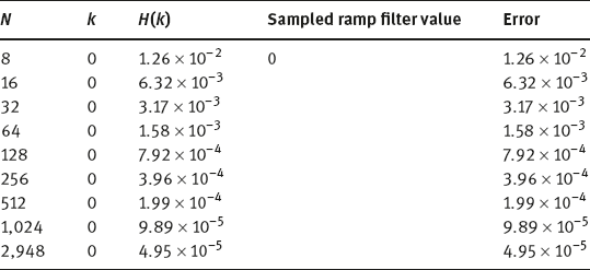
Errors may occur if the sampled continuous ramp filter is used. The errors are expressed as

$\text{Erorr}\left(\omega =\frac{k}{M}\right)=H(k)-\frac{\left|k\right|}{M},\text{for}\frac{\left|k\right|}{M}\le \mathrm{0.5.}$

Some numerical values according to eq. (2.60) are listed in Tables 2.1 and 2.2 with M =2N. It is observed from Tables 2.1 and 2.2 that if one uses the directly sampled ramp filter in DFT or FFT implementation, the DC gain needs to be corrected, while the errors for other frequency gains are small enough and can be ignored when the size M is large.

Tab. 2.1: Errors for ω = 0, M = 2N.

Tab. 2.2: Errors for ω = 1/16 = 0.0625, M = 2N.

Example 5: Use MATLAB to numerically evaluate the 1,024-point-induced ramp filter H by the kernel h defined in eq. (2.55). What is the DC gain of this induced ramp filter?

Solution

The MATLAB code is given as follows.

The results are plotted below, and the value of DC gain is 9.8946 × 10–5.

2.8Summary

–The Fourier transform is a useful tool to express a function in the frequency domain. The inverse Fourier transform brings the frequency representation back to the original spatial domain expression.

–In the Fourier domain, the projection data and the original image are clearly related. This relationship is stated in the popular central slice theorem. The 1D Fourier transform of the projection data at one view is one line in the 2D Fourier transform of the original image. Once we have a sufficient number of projection view angles, their corresponding lines will cover the 2D Fourier plane.

–The backprojection pattern in the 2D Fourier domain indicates that the sampling density is proportional to 1/|ω|. Therefore, the backprojection itself can only provide a blurred reconstruction. An exact reconstruction requires a combination of ramp filtering and backprojection.

–The most popular image reconstruction algorithm is the FBP algorithm. The ramp filtering can be implemented as multiplication in the frequency domain or as convolution in the spatial domain.

–One has the freedom to switch the order of ramp filtering and backprojection.

–Ramp filtering can be further decomposed to the Hilbert transform and the derivative operation. Therefore, we have even more ways to reconstruct the image.

–Under certain conditions, the ROI can be exactly reconstructed with truncated projection data.

–The readers are expected to understand two main concepts in this chapter: the central slice theorem and the FBP algorithm.

Problems

Problem 2.1	Let a 2D object be defined as $f(x,y)=\cos (2\pi x)+\cos (2\pi y).$ Find its 2D Fourier transform F(ωx, ωy). Determine the Radon transform of this object f(x, y) using the central slice theorem.
Problem 2.2	Let f1(x, y) and f2(x, y) be two 2D functions, and their Radon transforms are p1(s, θ) and p2(s, θ), respectively. If f(x, y) is the 2D convolution of f1(x, y) and f2(x, y), use the central slice theorem to prove that the Radon transform of f(x, y) is the convolution of p1(s, θ) and p2(s, θ) with respect to variable s.
Problem 2.3	Let the Radon transform of a 2D object f(x, y) be p(s, θ), the 2D Fourier transform of f(x, y) be F(ωx, ωy), and the 1D Fourier transform of p(s, θ) with respect to the first variable s be P(ω, θ). What is the physical meaning of the value F(0, 0)? What is the physical meaning of the value P(0, θ)? Is it possible that ${\displaystyle \underset{-\infty }{\overset{\infty }{\int }}g(s,0^{\circ })}\text{d}s\ne {\displaystyle \underset{-\infty }{\overset{\infty }{\int }}g(s,{90}^{\circ })}ds?$
Problem 2.4	Prove that the Hilbert transform of the function $\begin{array}{l}\text{is}f(t)=\{\begin{array}{l}\sqrt{1-t^2},\left|t\right|<1\\ 0,\left|t\right|1\end{array}\\ g(t)=\{\begin{array}{l}t,\left|t\right|<1\\ t-\sqrt{t^2-1}\mathrm{sgn}(t),\left|t\right|\ge 1.\end{array}\end{array}$

Bibliography

[1]Bracewell RN (1956) Strip integration in radio astronomy. Aust J Phys 9:198–217.

[2]Bracewell RN (1986) The Fourier Transform and its Applications, 2nd ed., McGraw-Hill, New York.

[3]Carrier GF, Krook M, Pearson CE (1983) Functions of a Complex Variable Theory and Technique, Hod, Ithaca.

[4]Clackdoyle R, Noo F, Guo J, Roberts J (2004) A quantitative reconstruction from truncated projections of compact support. Inverse Probl 20:1281–1291.

[5]Deans SR (1983) The Radon Transform and Some of Its Applications. John Wiley & Sons, New York.

[6]Defrise M, Noo F, Clackdoyle, Kudo H (2006) Truncated Hilbert transform and image reconstruction from limited tomographic data. Inverse Probl 22:1037–1053.

[7]Hahn SL (1996) Hilbert Transforms in Signal Processing, Artech House, Boston.

[8]Huang Q, Zeng GL, Gullberg GT (2007) An analytical inversion of the 180° exponential Radon transform with a numerically generated kernel. Int J Image Graphics 7:71–85.

[9]Kak AC, Slaney M (1998) Principles of Computerized Tomographic Imaging, IEEE Press, New York.

[10]Kanwal RP (1971) Linear Integral Equations Theory and Technique, Academic Press, New York.

[11]Natterer F (1986) The Mathematics of Computerized Tomography, Wiley, New York.

[12]Noo F, Clackdoyle R, Pack JD (2004) A two-step Hilbert transform method for 2D image reconstruction. Phys Med Biol 49:3903–3923.

[13]Sidky EY, Pan X (2005) Recovering a compactly supported function from knowledge of its Hilbert transform on a finite interval. IEEE Trans Signal Process Lett 12:97–100.

[14]Shepp L, Logan B (1974) The Fourier reconstruction of a head section. IEEE Trans Nucl Sci 21:21–43.

[15]Tricomi FG (1957) Integral Equations, Interscience, New York

[16]Ye Y, Yu H, Wei Y, Wang G (2007) A general local reconstruction approach based on a truncated Hilbert transform. Int J Biom Imag 63634.

[17]Ye Y, Yu H, Wang G (2007) Exact interior reconstruction with cone-beam CT. Int J Biom Imag 10693.

[18]You J, Zeng GL (2006) Exact finite inverse Hilbert transforms. Inverse Probl 22:L7–L10.

[19]Yu H, Yang J, Jiang M, Wang G (2009) Interior SPECT - exact and stable ROI reconstruction from uniformly attenuated local projections. Commun Numer Methods Eng 25:693–710.

[20]Yu H, Ye Y, Wang G (2008) Interior reconstruction using the truncated Hilbert transform via singular value decomposition. J X-Ray Sci Tech 16:243–251.

[23]Zeng GL (2007) Image reconstruction via the finite Hilbert transform of the derivative of the backprojection. Med Phys 34:2837–2843.

[22]Zeng GL (2015) Re-visit of the ramp filter. IEEE Trans Nucl Sci 62:131–136.

[23]Zeng GL, You J, Huang Q, Gullberg GT (2007) Two finite inverse Hilbert transform formulae for local tomography. Int J Imag Syst Tech 17:219–223.