3Fan-beam image reconstruction

The image reconstruction algorithms discussed in Chapter 2 are for parallel-beam imaging. If the data acquisition system produces projections that are not along parallel lines, the image reconstruction algorithms presented in Chapter 2 cannot be applied directly. This chapter uses the flat detector and curved detector fan-beam imaging geometries to illustrate how a parallel-beam reconstruction algorithm can be converted to user’s imaging geometry for image reconstruction.

3.1Fan-beam geometry and the point spread function

The fan-beam imaging geometry is common in X-ray computed tomography (CT), where the fan-beam focal point is the X-ray source. A fan-beam imaging geometry and a parallel-beam imaging geometry are compared in Figure 3.1.

For the parallel-beam geometry, we have a central slice theorem to derive reconstruction algorithms. We do not have an equivalent theorem for the fan-beam geometry. We will use a different strategy – converting the fan-beam imaging situation into the parallel-beam imaging situation and modifying the parallel-beam algorithms for fan-beam use.

In Chapter 2, when we discussed parallel-beam imaging problems, it was not mentioned, but we always assumed that the detector rotates around at a constant speed and has a uniform angular interval when data are taken. We make the same assumption here for the fan beam.

For the parallel-beam imaging geometry, this assumption results in a shift-invariant point spread function (PSF) for projection/backprojection. In other words, if you put a point source in the x–y plane (it does not matter where you put it), calculate the projections, and perform the backprojection, then you will always get the same star-like pattern (see Figure 3.2). This pattern is called the point spread function of the projection/backprojection operation.

In the parallel-beam case, when you find the backprojection at the point (x, y), you draw a line through this point and perpendicular to each detector. This line meets the detector at a point, say, s∗. Then add the value p(s∗, θ) to the location (x, y).

In the fan-beam case, when you find the backprojection at the point (x, y), you draw a line through this point and each focal-point location. This line has an angle, say, γ∗, with respect to the central ray of the detector. Then add the value g(γ∗, β) to location (x, y).

It can be shown that if the fan-beam focal-point trajectory is a complete circle, the PSF is shift invariant (i.e., the pattern does not change when the location of the point source changes) and has the same PSF pattern as that for the parallel-beam case (see Figure 3.3).

Fig. 3.1: Comparison of the parallel-beam and the fan-beam imaging geometries.

This observation is important. It implies that if you project and backproject an image, you will get the same blurred version of that image, regardless of the use of parallel-beam or fan-beam geometry.

If the original image is f(x, y) and if the backprojection of the projection data is b(x, y), then the PSF can be shown to be 1/r, where r = $r=\sqrt{x^2+y^2}.\text{Then}\text{f(}x,y\text{)}$ and b(x, y) are related by

$b(x,y)=f(x,y)\ast \ast \frac{1}{r},$

Fig. 3.2: The projection/backprojection PSF is shift invariant.

Fig. 3.3: The fan-beam 360° full-scan PSF is the same as that for the parallel-beam scan.

where “ ∗∗” denotes 2D convolution. The Fourier transform of b is B, and the Fourier transform of f is F. Thus the above relationship in the Fourier domain becomes

$B({\omega }_x,{\omega }_y)=F({\omega }_x,{\omega }_y)\times \frac{1}{\sqrt{({\omega }_x^2,{\omega }_y^2)}},$

because the 2D Fourier transform of $1/\sqrt{x^2+y^2}\text{is1/}\sqrt{{\omega }_x^2+{\omega }_y^2}.$

We already know that if a 2D ramp filter is applied to the backprojected image b(x, y), the original image f(x, y) can be obtained. The same technique can be used for the fan-beam backprojected image b(x, y). The backprojection-then-filtering algorithm is the same for the parallel-beam and fan-beam imaging geometries. If we apply the 2D ramp filter $\sqrt{{\omega }_x^2+{\omega }_y^2}$ to both sides of the above Fourier domain relationship, the Fourier transform F(ωx, ωy) of the original image f(x, y) is readily obtained:

$F({\omega }_x,{\omega }_y)=B({\omega }_x,{\omega }_y)\times \sqrt{{\omega }_x^2+{\omega }_y^2}.$

Finally, the original image f(x, y) is found by taking the 2D inverse Fourier transform.

3.2Parallel-beam to fan-beam algorithm conversion

If you want to reconstruct the image by a filter-then-backproject (i.e., filtered backprojection [FBP]) algorithm, a different strategy must be used.

A straightforward approach would be to rebin every fan-beam ray into a parallel-beam ray. For each fan-beam ray sum g(γ, β), we can find a parallel-beam ray sum p(s, θ) that has the same orientation as the fan-beam ray with the relations (see Figure 3.4)

$\theta =\gamma +\beta ,$

and

$s=D\sin \gamma ,$

where D is the focal length. We then assign

$p(s,\theta )=g(\gamma ,\beta ).$

After rebinning the fan-beam data into the parallel-beam format, we then use a parallel-beam image reconstruction algorithm to reconstruct the image. However, this rebinning approach is not preferred because rebinning requires data interpolation when changing coordinates. Data interpolation introduces errors. The idea of rebinning is feasible, but the results may not be accurate enough.

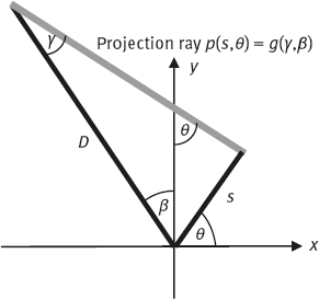
Fig. 3.4: A fan-beam ray can be represented using the parallel-beam geometry parameters.

However, the idea above is not totally useless. Let us do it in a slightly different way. We start out with a parallel-beam image reconstruction algorithm, which is a mathematical expression. On the left-hand side of the expression is the reconstructed image f(x, y). On the right-hand side is an integral expression that contains the projection p(s, θ) and some other factors associated with s and θ (see Figure 3.5).

Next, we replace the parallel-beam projection p(s, θ) by its equivalent fan-beam counterpart g(γ, β) on the right-hand side. Of course, this substitution is possible only if the conditions θ = γ + β and s = D sin γ are satisfied. These two relations are easier to see in Figure 3.4, which is derived from Figure 3.1.

In order to satisfy these two conditions, we stick them into the right-hand side of the expression. This procedure is nothing but changing the variables in the integral, where the variables s and θ are changed into γ and β.

As a reminder, in calculus, when you change the variables in an integral, you need a Jacobian factor, which is a determinant calculated with some partial derivatives. This Jacobian is a function of γ and β.

Fig. 3.5: The procedure to change a parallel-beam algorithm into a fan-beam algorithm.

Fig. 3.6: Flat and curved detector fan-beam geometries.

After substituting the parallel-beam data p(s, θ) with fan-beam data g(γ, β), changing variables s and θ to γ and β, and inserting a Jacobian J(γ, β), a new fan-beam image reconstruction algorithm is born (see Figure 3.5)!

The method outlined in Figure 3.5 is generic. We have a long list of parallel-beam image reconstruction algorithms. They can all be converted into fan-beam algorithms in this way, and accordingly, we also have a long list of fan-beam algorithms. We must point out that after changing the variables, a convolution operation (with respect to variable s) may not turn into a convolution (with respect to variable γ) automatically, and some mathematical manipulation is needed to turn it into a convolution form. Like parallel-beam algorithms, the fan-beam algorithms include combinations of ramp filtering and backprojection or combinations of the derivative, Hilbert transform, and backprojection (DHB).

Researchers treat the flat detector fan-beam and curved detector fan-beam differently in reconstruction algorithm development. In a flat detector, the data points are sampled with equal distance Δs intervals, while in a curved detector, the data points are sampled with equal angle Δ γ intervals (see Figure 3.6). A fan-beam algorithm can be converted from one geometry to the other with proper weighting adjustments.

3.3Short scan

In parallel-beam imaging, when the detector rotates 2π (i.e., 360°), each projection ray is measured twice, and the redundant data are related by

$p(s,\theta )=p(-s,\theta +\pi );$

the redundant data are acquired by the two face-to-face detectors (see Figure 3.7). Therefore, it is sufficient to acquire data over an angular range of π.

Fig. 3.7: Face-to-face parallel-beam detectors measure the same line integrals.

Fig. 3.8: Each ray is measured twice in a fan-beam 360° full scan.

Likewise, when the fan-beam detector rotates 2π, each projection ray is also measured twice, and the redundant data are related by (see Figure 3.8)

$g(\gamma ,\beta )=g(-\gamma ,\beta +2\gamma +\pi ).$

Due to data redundancy, we can use a smaller angular (β) range than 2π for fan-beam data acquisition, hence the term short scan. The minimal range of β is determined by how the data are acquired. This required range can be less than π (see Figure 3.9, left), equal to π (see Figure 3.9, middle), or larger than π (see Figure 3.9, right). The criterion is that we need at least 180° angular coverage for each point in the object in which we are interested.

Fig. 3.9: Fan-beam minimum scan angle depends on the location of the object.

Fig. 3.10: For a fan-beam short scan, some rays are measured once and some rays are measured twice.

We need to be cautious that in a fan-beam short scan, some rays are measured once, and other rays are measured twice. Even for the case that the angular range of β is less than π, there are still rays that are measured twice. In fact, any ray that intersects the measured focal-point trajectory twice is measured twice (see Figure 3.10). We require that any ray which passes through the object should be measured at least once. Proper weighting should be used in image reconstruction if data are redundant. For example, if a ray is measured twice, the sum of the weighting factors for these two measurements should be unity. For a fan-beam short scan, the projection/backprojection PSF is no longer shift invariant.

3.4Mathematical expressions

This section presents the derivation steps for the FBP algorithm for the curved fan-beam detector. The ramp filter used in the filtering step is formulated as a convolution. In this algorithm, the fan-beam backprojector contains a distance-dependent weighting factor, which causes nonuniform resolution throughout the reconstructed image when a window function is applied to the ramp filter in practice. In order to overcome this problem, the ramp filter can be replaced by a derivative operation and the Hilbert transform. The derivation of the fan-beam algorithm using the derivative and the Hilbert transform is given in this section.

3.4.1Derivation of a filtered backprojection fan-beam algorithm

We begin with the parallel-beam FBP algorithm (see Section 2.6.5), using polar coordinates (r, φ) instead of Cartesian coordinates (x, y). Then x = r cos y, y = r sin y, and x cos θ + y sin θ = r cos(θ – y). We have

$f(r,\phi )=\frac{1}{2}{\displaystyle \underset{0}{\overset{2\pi }{\int }}{\displaystyle \underset{-\infty }{\overset{\infty }{\int }}p(s,\theta )}}h(r\cos (\theta -\phi )-s)dsd\theta .$

Changing variables θ = γ + β and s = D sin γ with the Jacobian D cos γ yields

$f(r,\phi )=\frac{1}{2}{\displaystyle \underset{0}{\overset{2\pi }{\int }}{\displaystyle \underset{-\pi /2}{\overset{\pi /2}{\int }}g(\gamma ,\beta )h(r\cos (\beta +\gamma -\phi )}}-D\sin \gamma )D\cos \gamma d\gamma d\beta .$

This is a fan-beam reconstruction algorithm, but the inner integral over γ is not yet in the convolution form. Convolution is much more efficient than a general integral in implementation. In the following, we are going to convert the integral over γ to a convolution with respect to γ.

For a given reconstruction point (r, φ), we define D′ and γ′ as shown in Figure 3.11, then r cos(β + γ – φ)– D sin γ = D′ sin(γ′ – γ), and

$f(r,\phi )=\frac{1}{2}{\displaystyle \underset{0}{\overset{2\pi }{\int }}{\displaystyle \underset{-\pi /2}{\overset{\pi /2}{\int }}g(\gamma ,\beta )h(D^{\prime }\sin ({\gamma }^{\prime }-\gamma ))D\cos \gamma d\gamma d\beta .}}$

Now, we prove a special property of the ramp filter

$h\left(D\text{'}\sin \gamma \right)={\left(\frac{\gamma }{D\text{'}\sin \gamma }\right)}^{2}h\left(\gamma \right),$

which will be used in the very last step, the derivation, of the fan-beam formula.

Fig. 3.11: The reconstruction point (r, y) defines the angle γγ and distance Dγ.

Using the definition of the ramp filter kernel $h\left(t\right)={\displaystyle \underset{-\infty }{\overset{\infty }{\int }}\left|\omega \right|e^{i2\omega t}d\omega },$ we have

$\begin{array}{l}h\left(D\text{'}\sin \gamma \right)={\displaystyle \underset{-\infty }{\overset{\infty }{\int }}\left|\omega \right|e^{i2\pi D\text{'}\sin \gamma }d\omega }\\ ={\left(\frac{\gamma }{D\text{'}\sin \gamma }\right)}^2{\displaystyle \underset{-\infty }{\overset{\infty }{\int }}\left|\omega D\text{'}\frac{\sin \gamma }{\gamma }\right|}{e}^{i2\pi \omega \frac{D\text{'}\sin \gamma }{\gamma }\gamma }d\left(\omega D\text{'}\frac{\mathrm{Sin}\gamma }{\gamma }\right)\\ ={\left(\frac{\gamma }{D\text{'}\sin \gamma }\right)}^2{\displaystyle \underset{-\infty }{\overset{\infty }{\int }}\left|\widehat{\omega }\right|}{e}^{i2\pi \omega \gamma }d\widehat{\omega }\\ ={\left(\frac{\gamma }{D\text{'}\sin \gamma }\right)}^{2}h\left(\gamma \right).\end{array}$

If we denote hfan(γ)= (D/2) (γ/sin γ)2 h(γ), then the fan-beam convolution backprojection algorithm is obtained as

$f\left(r,\phi \right)={\displaystyle \underset{0}{\overset{2\pi }{\int }}\frac{1}{{\left(D\text{'}\right)}^2}}{\displaystyle \underset{-\pi /2}{\overset{\pi /2}{\int }}\left(\cos \gamma \right)g\left(\gamma ,\beta \right)h_{\text{fan}}\left(\gamma \text{'}-\gamma \right)d\gamma d\beta .}$

3.4.2A fan-beam algorithm using the derivative and the Hilbert transform

The general idea of decomposition of the ramp filter into the derivative and the Hilbert transform can be applied to fan-beam image reconstruction. A derivative– Hilbert transform–backprojection algorithm can be obtained by doing a coordinate transformation on the Radon inversion formula (see Section 2.6.6) as follows. Noo, Defrise, Kudo, Clackdoyle, Pan, Chen, Wang, You, and many others have contributed significantly in developing algorithms using the derivative and the Hilbert transform. We first rewrite the Radon inversion formula (see Section 2.6.6) in the polar coordinate system, that is, f(r, φ) can be reconstructed as

$f\left(r,\phi \right)=\frac{1}{2}{\displaystyle \underset{0}{\overset{2\pi }{\int }}{\displaystyle \underset{-\infty }{\overset{\infty }{\int }}\frac{\partial p\left(s,\theta \right)}{\partial s}\frac{1}{2{\pi }^2\left(r\cos \left(\theta -\phi \right)-s\right)}dsd\theta .}}$

Changing variables from (s, θ) to(γ, β) and using $\frac{\partial p}{\partial s}=\frac{1}{D\cos \gamma }\frac{\partial g}{\partial \gamma },$ we have

$\begin{array}{l}f\left(r,\phi \right)=\frac{1}{2}{\displaystyle \underset{0}{\overset{2\pi }{\int }}{\displaystyle \underset{-\pi /2}{\overset{\pi /2}{\int }}\frac{1}{D\cos \gamma }}}\frac{\partial g\left(\gamma ,\beta \right)}{\partial \gamma }\frac{1}{2{\pi }^{2}D\text{'}\sin \left(\gamma \text{'}-\gamma \right)}D\cos \gamma d\gamma d\beta \\ ={\displaystyle \underset{0}{\overset{2\pi }{\int }}\frac{1}{4{\pi }^{2}D\text{'}}}{\displaystyle \underset{-\pi /2}{\overset{\pi /2}{\int }}\frac{\partial g\left(\gamma ,\beta \right)}{\partial \gamma }\frac{1}{\sin \left(\gamma \text{'}-\gamma \right)}}d\gamma d\beta ,\end{array}$

where D' is the distance from the reconstruction point to the focal point at angle β. This D' factor is not desirable in a reconstruction algorithm. A small D' can make the algorithm unstable; this spatially variant factor also costs some computation time. In a 2π scan, each ray is measured twice. If proper weighting is chosen for the redundant measurements, this D' factor can be eliminated.

Let us introduce a weighting function w in the above DHB algorithm:

$f\left(r,\phi \right)=\frac{1}{4{\pi }^2}{\displaystyle \underset{0}{\overset{2\pi }{\int }}\frac{w\left(\gamma \text{'},\beta ,r,\phi \right)}{D\text{'}}{\displaystyle \underset{-\pi /2}{\overset{\pi /2}{\int }}\left(\frac{\partial }{\partial \gamma }+\frac{\partial }{\partial \beta }\right)g\left(\gamma ,\beta \right)\frac{1}{\sin \left(\gamma \text{'}-\gamma \right)}d\gamma d\beta }}.$

If we use g to denote the result of the derivative and Hilbert transform of the fan-beam data:

$\widehat{g}\left(\gamma \text{'},\beta \right)={\displaystyle \underset{-\pi /2}{\overset{\pi /2}{\int }}\left(\frac{\partial }{\partial \gamma }+\frac{\partial }{\partial \beta }\right)}g\left(\gamma ,\beta \right)\frac{1}{\sin \left(\gamma \text{'}-\gamma \right)}d\gamma ,$

then

$f\left(r,\phi \right)=\frac{1}{4{\pi }^2}{\displaystyle \underset{0}{\overset{2\pi }{\int }}\frac{w\left(\gamma \text{'},\beta ,r,\phi \right)}{D\text{'}}\widehat{g}\left(\gamma \text{'},\beta \right)d\beta .}$

It can be shown that g/D' has the same redundancy property as the original fan-beam data g (see Figure 3.8). Therefore, it is required that the weighting function satisfies the condition

$w\left(\gamma \text{'},\beta ,r,\phi \right)+w\left({\gamma }_c^{\text{'}},{\beta }_c,r,\phi \right)=2$

Fig. 3.12: Proper weighting can make the distance-dependent factor disappear from the backprojector in a 360° full scan.

with ${\gamma }_c^{\text{'}}=-{\gamma }^{\text{'}}\text{and}{\beta }_c=\beta +2\gamma \text{'}+\pi .$ If we define $w\left(\gamma \text{'},\beta ,r,\phi \right)=D\text{'}/\left(D\cos \gamma \text{'}\right),$ then the above condition is satisfied because $D\text{'}+D_c^{\text{'}}=2D\cos \gamma \text{'}$(see Figure 3.12). Finally,

$\begin{array}{l}f\left(r,\phi \right)=\frac{1}{2}\left\{\frac{1}{4{\pi }^2}{\displaystyle \underset{0}{\overset{2\pi }{\int }}\left[\frac{w\left(\gamma \text{'},\beta ,r,\phi \right)}{D\text{'}}+\frac{w\left({\gamma }_c^{\text{'}},{\beta }_c,r,\phi \right)}{D_c^{\text{'}}}\right]}\widehat{g}\left(\gamma \text{'},\beta \right)d\beta \right\}\\ =\frac{1}{4{\pi }^{2}D}{\displaystyle \underset{0}{\overset{2\pi }{\int }}\frac{1}{\cos \gamma \text{'}}\widehat{g}\left(\gamma \text{'},\beta \right)d\beta }\end{array}$

This result can be derived without introducing a weighting function w (see a paper listed at the end of this chapter by You and Zeng).

3.4.3Expression for the Parker weights

Short scan in fan-beam tomography has wide applications in industry and health care; it can acquire sufficient line-integral measurements by scanning the object 180° plus the full fan angle.

In short-scan fan-beam imaging, the projections g(γ, β) are acquired when the fan-beam rotation angle β is in the range of [0°,180° +2δ] or in a larger range, where δ is half of the fan angle. The redundant measurements in the range of [0°,180° +2δ]are weighted by the Parker weights:

$w\left(\gamma ,\beta \right)=\{\begin{array}{c}{\sin }^2\left(\frac{\pi }{4}\frac{\pi +2\delta -\beta }{\delta +\gamma }\right),\\ {\sin }^2\left(\frac{\pi }{4}\frac{\beta }{\delta +\gamma }\right),\\ 1,\end{array}\begin{array}{c}\text{if}\\ \text{if}\\ \text{otherwise}\text{.}\end{array}\begin{array}{c}\pi -2\delta \le \beta \le \pi +2\delta \text{and}\text{0}\le \frac{\pi +2\delta -\beta }{\delta +\gamma }\le 2,\\ 0\le \beta \le 4\delta \text{and}\text{0}\le \frac{\beta }{\delta -\gamma }\le 2,\end{array}$

One then uses the scaled fan-beam projections w(γ, β)g(γ, β) inplace of g(γ, β) in the fan-beam FBP image reconstruction algorithm.

Short-scan weighting is not unique. A function w(γ, β) is a valid short-scan weighting function as long as it satisfies

$w\left(\gamma ,\beta \right)+w\left(-\gamma ,\beta +2\gamma +\pi \right)=1.$

For discrete data, the weighting function w(γ, β) must be very smooth, otherwise artifacts will appear. If the weighting function is not smooth enough, a sudden change in the projections can cause a spike in the ramp-filtered projections. In an ideal situation, an opposite spike will also be created and this opposite spike should be able to cancel the other spike. When data are discretely sampled, the positive spike and the negative spike do not match well. The uncanceled residue causes image artifacts. The main strategy of Parker’s method is to make the weighting function as smooth as possible, so that the weighting function does not introduce any undesired components.

3.4.4Errors caused by finite bandwidth implementation

In the derivation of the fan-beam FBP algorithm in Section 3.4.1, the bandwidth of the ramp filter is assumed to be infinity:

$h\left(\gamma \right)={\displaystyle \underset{-\infty }{\overset{\infty }{\int }}\left|\omega \right|}{e}^{i2\pi \omega \gamma }d\omega .$

It has a property that

$h\left(a\gamma \right)={\displaystyle \underset{-\infty }{\overset{\infty }{\int }}\left|\omega \right|}{e}^{i2\pi \omega a\gamma }d\omega =\frac{1}{a^2}h\left(\gamma \right).$

In practice, the data are discretely sampled and the bandwidth is bounded. The band-limited ramp filter is expressed as

$h_{\Omega }\left(\gamma \right)={\displaystyle \underset{-\Omega }{\overset{\Omega }{\int }}\left|\omega \right|}{e}^{i2\pi \omega \gamma }d\omega .$

Let x = aω and we have

$h_{\Omega }\left(a\gamma \right)=\frac{1}{a^2}{\displaystyle \underset{-a\Omega }{\overset{a\Omega }{\int }}\left|x\right|}{e}^{i2\pi x\gamma }dx=\frac{1}{a^2}{h}_{a\Omega \left(\gamma \right)\ne }\frac{1}{a^2}{h}_{\Omega \left(\gamma \right)}.$

Therefore, for band-limited fan-beam data the derivation of the fan-beam FBP algorithm in Section 3.4.1 is not valid. Fortunately, for the full-scan fan-beam projections, the errors in the FBP reconstruction are not significant and are usually not noticeable. However, the errors can be significant for short-scan fan-beam data when the fan-beam focal length is short and the Parker weights are used. Figure 3.13 illustrates a short-scan fan-beam FBP reconstruction when a short focal length of 270 units is used. The object is a uniform disc with a radius of 230 units. The true image value within the disc is 1. The image display window is [0.76, 1.57].

Fig. 3.13: A short-scan fan-beam FBP reconstruction of a uniform disc, when the fan-beam focal length is very short.

Fig. 3.14: A three-piece fan-beam focal-point trajectory.

3.5Worked examples

Example 1: Does the following fan-beam geometry acquire sufficient projection data for image reconstruction? The fan-beam focal-point trajectory consists of three disjoint arcs as shown in Figure 3.14.

Solution

Yes. If you draw any line through the circular object, this line will intersect the focal-point trajectory at least once.

Fig. 3.15: A redundant measurement in a fan-beam scan.

Example 2: On the γ–β plane (similar to the sinogram for the parallel-beam projections), identify the double measurements for a fan-beam 2π scan.

Solution

From Figure 3.15, we can readily find the fan-beam data redundancy conditions for

$g\left({\gamma }_1,{\beta }_1\right)=g\left({\gamma }_2,{\beta }_2\right)$

as

${\gamma }_2=-{\gamma }_1$

and

${\beta }_2={\beta }_1+2{\gamma }_1+\pi .$

Using these conditions, the fan-beam data redundancy is depicted on the γ–β plane in Figure 3.16, where every vertical line corresponds to a redundant slant line.

Fig. 3.16: In the γ–β plane representation of the fan-beam data, each vertical line of measurements is the same as the slant line of measurements with the same color.

Example 3: Derive a FBP algorithm for the flat-detector fan-beam geometry.

Solution

We begin with the parallel-beam FBP algorithm, using polar coordinates (r, φ) instead of Cartesian coordinates (x, y). Then x = r cos φ, y = r sin φ, and x cos θ + y sin θ = r cos(θ – φ). We have

$f\left(r,\phi \right)=\frac{1}{2}{\displaystyle \underset{0}{\overset{2\pi }{\int }}{\displaystyle \underset{-\infty }{\overset{\infty }{\int }}p\left(s,\theta \right)h\left(r\cos \left(\theta -\phi \right)-s\right)dsd\theta .}}$

For the flat-detector fan-beam projection g(t, β)= p(s, θ), the fan-beam and parallel-beam variables are related by θ = β +tan–1 (t) and $s=D\left(t/\sqrt{D^2+t^2}\right).$ Changing the parallel-beam variables to the fan-beam variables with the Jacobian D3 /(D2 + t2)3/2 /D yields

$f\left(r,\phi \right)=\frac{1}{2}{\displaystyle \underset{0}{\overset{2\pi }{\int }}{\displaystyle \underset{-\infty }{\overset{\infty }{\int }}g\left(t,\beta \right)h}}\left(\left(\widehat{t}-t\right)\frac{UD}{\sqrt{D^2+t^2}}\right)\frac{D^3}{{\left(D^2+t^2\right)}^{3/2}}dtd\beta ,$

where we have used $r\cos \left(\theta -\phi \right)-s=\left(\widehat{t}-t\right)\left(UD/\sqrt{D^2+t^2}\right)$ with

$U=\frac{D+r\sin \left(\beta -\phi \right)}{D}$

and

$\widehat{t}=\frac{Dr\cos \left(\beta -\phi \right)}{D+r\sin \left(\beta -\phi \right)}$

(see Figure 3.17).

Fig. 3.17: Notation for flat detector fan-beam imaging geometry.

This is a fan-beam reconstruction algorithm, but the inner integral over t is not yet in the convolution form. Using a special property of the ramp filter h(at)= (1 /a2 ) h(t) yields

$f\left(r,\phi \right)=\frac{1}{2}{\displaystyle \underset{0}{\overset{2\pi }{\int }}\frac{1}{U^2}}{\displaystyle \underset{-\infty }{\overset{\infty }{\int }}\frac{D}{\sqrt{D^2+t^2}}g\left(t,\beta \right)h\left(\widehat{t}-t\right)}dtd\beta .$

This is a fan-beam convolution backprojection algorithm, where $D/\sqrt{D^2+t^2}$ is the cosine pre-weighting factor, the integral over t is the ramp-filter convolution, and 1/U2 is the distance-dependent weighting factor in the backprojection.

Note: The relationship $h\left(at\right)=\left(1/a^2\right)h\left(t\right)$ does not hold for a windowed ramp filter. Therefore, the fan-beam algorithm derived above does not have uniform resolution in the reconstructed image in practice when a window function is applied to the ramp filter.

3.6Summary

–The fan-beam geometry is popular in X-ray CT imaging.

–The fan-beam image reconstruction algorithms can be derived from their parallel-beam counterparts via changing of variables.

–There are two types of fan-beam detectors, that is, the flat detectors and curved detectors. Each detector type has its own image reconstruction algorithms.

–If the fan-beam focal-point trajectory is a full circle, it is called full scan. If the trajectory is a partial circle, it is called short scan. Even for a short scan, some of the fan-beam rays are measured twice. The redundant measurements need proper weighting during image reconstruction.

–For some fan-beam image reconstruction algorithms, the backprojector contains a distance-dependent weighting factor. When a window function is applied to the ramp filter, this factor is not properly treated by the window function and the resultant fan-beam FBP is no longer exact in the sense that the reconstructed image has nonuniform resolution and intensity. The short-scan fan-beam FBP algorithm can result in noticeable errors if the focal length is very short.

–The modern derivative and Hilbert transform-based algorithms are able to weigh the short-scan redundant data in a correct way.

–In this chapter, the readers are expected to understand how a fan-beam algorithm can be obtained from a parallel-beam algorithm.

Problems

Bibliography

[1]Besson G (1996) CT fan-beam parameterizations leading to shift-invariant filtering. Inverse Probl 12:815–833.

[2]Chen GH (2003) A new framework of image reconstruction from fan beam projections. Med Phys 30:1151–1161.

[3]Chen GH, Tokalkanajalli R, Hsieh J (2006) Development and evaluation of an exact fan-beam reconstruction algorithm using an equal weighting scheme via locally compensated filtered backprojection (LCFBP). Med Phys 33:475–481.

[4]Dennerlein F, Noo F, Hornegger J, Lauritsch G (2007) Fan-beam filtered-backprojection reconstruction without backprojection weight. Phys Med Biol 52:3227–3240.

[5]Gullberg GT (1979) The reconstruction of fan-beam data by filtering the back-projection. Comput Graph Image Process 10:30–47.

[6]Hanajer C, Smith KT, Solmon DC, Wagner SL (1980) The divergent beam X-ray transform. Rocky Mt J Math 10:253–283.

[7]Natterer N (1993) Sampling in fan-beam tomography. SIAM J Appl Math 53:358–380.

[8]Horn BKP (1979) Fan-beam reconstruction methods. Proc IEEE 67:1616–1623.

[9]Noo F, Defrise M, Clackdoyle R, Kudo H (2002) Image reconstruction from fan-beam projections on less than a short scan. Phys Med Biol 47:2525–2546.

[10]Pan X (1999) Optimal noise control in and fast reconstruction of fan-beam computed tomography image. Med Phys 26:689–697.

[11]Pan X, Yu L (2003) Image reconstruction with shift-variant filtration and its implication for noise and resolution properties in fan-beam tomography. Med Phys 30:590–600.

[12]Parker DL (1982) Optimal short scan convolution reconstruction for fan beam CT. Med Phys 9:254–257.

[13]Silver MD (2000) A method for including redundant data in computed tomography. Med Phys 27:773–774.

[14]You J, Liang Z, Zeng GL (1999) A unified reconstruction framework for both parallel-beam and variable focal-length fan-beam collimators by a Cormack-type inversion of exponential Radon transform. IEEE Trans Med Imaging 18:59–65.

[15]You J, Zeng GL (2007) Hilbert transform based FBP algorithm for fan-beam CT full and partial scans. IEEE Trans Med Imaging 26:190–199.

[16]Yu L, Pan X (2003) Half-scan fan-beam computed tomography with improved noise and resolution properties. Med Phys 30:2629–2637.

[17]Wang J, Lu H, Li T, Liang Z (2005) An alternative solution to the nonuniform noise propagation problem in fan-beam FBP image reconstruction. Med Phys 32:3389–3394.

[18]Wei Y, Hsieh J, Wang G (2005) General formula for fan-beam computed tomography. Phys Rev Lett 95:258102.

[19]Wei Y, Wang G, Hsieh (2005) Relation between the filtered backprojection algorithm and the backprojection algorithm in CT. IEEE Signal Process Lett 12: 633–636.

[20]Wesarg S, Ebert M, and Bortfeld T (2002) Parker weights revisited. Med Phys 29:372–378Zeng GL (2004) Nonuniform noise propagation by using the ramp filter in fan-beam computed tomography. IEEE Trans Med Imaging 23:690–695.

[21]Zeng GL (2015) Fan-beam short-scan FBP algorithm is not exact. Phys Med Biol 60:N131–N139.

[22]Zeng GL, Gullberg (1991) Short-scan fan beam algorithm for non-circular detector orbits. SPIE Med Imaging V Conf, San Jose, CA, 332–340.

[23]Zou Y, Pan X, Sidky EY (2005) Image reconstruction in regions-of-interest from truncated projections in a reduced fan-beam scan. Phys Med Biol 50:13–28.