8
Multi-Factor Models
This chapter is devoted to estimating various factor models. Factors are variables/attributes that in the past were correlated with (then future) stock returns and are expected to contain the same predictive signals in the future.
These risk factors can be considered a tool for understanding the cross-section of (expected) returns. That is why various factor models are used to explain the excess returns (over the risk-free rate) of a certain portfolio or asset using one or more factors. We can think of the factors as the sources of risk that are the drivers of those excess returns. Each factor carries a risk premium and the overall portfolio/asset return is the weighted average of those premiums.
Factor models play a crucial role in portfolio management, mainly because:
- They can be used to identify interesting assets that can be added to the investment portfolio, which—in turn—should lead to better-performing portfolios.
- Estimating the exposure of a portfolio/asset to the factors allows for better risk management.
- We can use the models to assess the potential incremental value of adding a new risk factor.
- They make portfolio optimization easier, as summarizing the returns of many assets with a smaller number of factors reduces the amount of data required to estimate the covariance matrix.
- They can be used to assess a portfolio manager’s performance—whether the performance (relative to the benchmark) is due to asset selection and timing of the trades, or if it comes from the exposure to known return drivers (factors).
By the end of this chapter, we will have constructed some of the most popular factor models. We will start with the simplest, yet very popular, one-factor model (which is the same as the Capital Asset Pricing Model when the considered factor is the market return) and then explain how to estimate more advanced three-, four-, and five-factor models. We will also cover the interpretation of what these factors represent and give a high-level overview of how they are constructed.
In this chapter, we cover the following recipes:
- Estimating the CAPM
- Estimating the Fama-French three-factor model
- Estimating the rolling three-factor model on a portfolio of assets
- Estimating the four- and five-factor models
- Estimating cross-sectional factor models using the Fama-MacBeth regression
Estimating the CAPM
In this recipe, we learn how to estimate the famous Capital Asset Pricing Model (CAPM) and obtain the beta coefficient. This model represents the relationship between the expected return on a risky asset and the market risk (also known as systematic or undiversifiable risk). CAPM can be considered a one-factor model, on top of which more complex factor models were built.
CAPM is represented by the following equation:
![]()
Here, E(ri) denotes the expected return on asset i, rf is the risk-free rate (such as a government bond), E(rm) is the expected return on the market, and ![]() is the beta coefficient.
is the beta coefficient.
Beta can be interpreted as the level of the asset return’s sensitivity, as compared to the market in general. Below we mention the possible interpretations of the coefficient:
 <= -1: The asset moves in the opposite direction to the benchmark and in a greater amount than the negative of the benchmark.
- -1 < < 0: The asset moves in the opposite direction to the benchmark.
- = 0: There is no correlation between the asset’s price movement and the market benchmark.
- 0 < < 1: The asset moves in the same direction as the market, but the amount is smaller. An example might be the stock of a company that is not very susceptible to day-to-day fluctuations.
 = 1: The asset and the market are moving in the same direction by the same amount.
- > 1: The asset moves in the same direction as the market, but the amount is greater. An example might be the stock of a company that is very susceptible to day-to-day market news.
CAPM can also be represented as:
![]()
In this specification, the left-hand side of the equation can be interpreted as the risk premium, while the right-hand side contains the market premium. The same equation can be further reshaped into:
Here, ![]() and
and ![]() .
.
In this example, we consider the case of Amazon and assume that the S&P 500 index represents the market. We use 5 years (2016 to 2020) of monthly data to estimate the beta. In current times, the risk-free rate is so low that, for simplicity’s sake, we assume it is equal to zero.
How to do it...
Execute the following steps to implement the CAPM in Python:
- Import the libraries:
import pandas as pd import yfinance as yf import statsmodels.api as sm - Specify the risky asset, the benchmark, and the time horizon:
RISKY_ASSET = "AMZN" MARKET_BENCHMARK = "^GSPC" START_DATE = "2016-01-01" END_DATE = "2020-12-31" - Download the necessary data from Yahoo Finance:
df = yf.download([RISKY_ASSET, MARKET_BENCHMARK], start=START_DATE, end=END_DATE, adjusted=True, progress=False) - Resample to monthly data and calculate the simple returns:
X = ( df["Adj Close"] .rename(columns={RISKY_ASSET: "asset", MARKET_BENCHMARK: "market"}) .resample("M") .last() .pct_change() .dropna() ) - Calculate beta using the covariance approach:
covariance = X.cov().iloc[0,1]
benchmark_variance = X.market.var()
beta = covariance / benchmark_variance
The result of the code is
beta = 1.2035.
- Prepare the input and estimate the CAPM as a linear regression:
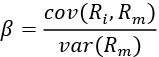
# separate target
y = X.pop("asset")
# add constant
X = sm.add_constant(X)
# define and fit the regression model
capm_model = sm.OLS(y, X).fit()
# print results
print(capm_model.summary())
Figure 8.1 shows the results of estimating the CAPM model:
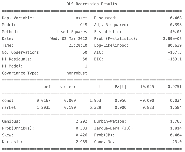
Figure 8.1: The summary of the CAPM estimated using OLS
These results indicate that the beta (denoted as the market here) is equal to 1.2, which means that Amazon’s returns are 20% more volatile than the market (proxied by S&P 500). Or in other words, Amazon’s (excess) return is expected to move 1.2 times the market (excess) return. The value of the intercept is relatively small and statistically insignificant at the 5% significance level.
How it works...
First, we specified the assets we wanted to use (Amazon and S&P 500) and the time frame. In Step 3, we downloaded the data from Yahoo Finance. Then, we only kept the last available price per month and calculated the monthly returns as the percentage change between the subsequent observations.
In Step 5, we calculated the beta as the ratio of the covariance between the risky asset and the benchmark to the benchmark’s variance.
In Step 6, we separated the target (Amazon’s stock returns) and the features (S&P 500 returns) using the pop method of a pandas DataFrame. Afterward, we added the constant to the features (effectively adding a column of ones to the DataFrame) with the add_constant function.
The idea behind adding the intercept to this regression is to investigate whether—after estimating the model—the intercept (in the case of the CAPM, also known as Jensen’s alpha) is zero. If it is positive and significant, it means that— assuming the CAPM model is true—the asset or portfolio generates abnormally high risk-adjusted returns. There are two possible implications: either the market is inefficient or there are some other undiscovered risk factors that should be included in the model. This issue is known as the joint hypothesis problem.
We can also use the formula notation, which adds the constant automatically. To do so, we must import statsmodels.formula.api as smf and then run the slightly modified line: capm_model = smf.ols(formula="asset ~ market", data=X).fit(). The results of both approaches are the same. You can find the complete code in the accompanying Jupyter notebook.
Lastly, we ran the OLS regression and printed the summary. Here, we could see that the coefficient by the market variable (that is, the CAPM beta) is equal to the beta that was calculated using the covariance between the asset and the market in Step 5.
There’s more...
In the example above, we assumed there was no risk-free rate, which is a reasonable assumption to make nowadays. However, there might be cases when we would like to account for a non-zero risk-free rate. To do so, we could use one of the following approaches.
Using data from Prof. Kenneth French’s website
The market premium (rm - rf ) and the risk-free rate (approximated by the one-month Treasury Bill) can be downloaded from Professor Kenneth French’s website (please refer to the See also section of this recipe for the link).
Please bear in mind that the definition of the market benchmark used by Prof. French is different from the S&P 500 index—a detailed description is available on his website. For a description of how to easily download the data, please refer to the Implementing the Fama-French three-factor model recipe.
Using the 13-Week T-bill
The second option is to approximate the risk-free rate with, for example, the 13-Week (3-month) Treasury Bill (Yahoo Finance ticker: ^IRX).
Follow these steps to learn how to download the data and convert it into the appropriate risk-free rate:
- Define the length of the period in days:
N_DAYS = 90 - Download the data from Yahoo Finance:
df_rf = yf.download("^IRX", start=START_DATE, end=END_DATE, progress=False) - Resample the data to monthly frequency (by taking the last value for each month):
rf = df_rf.resample("M").last().Close / 100 - Calculate the risk-free return (expressed as daily values) and convert the values to monthly:
rf = ( 1 / (1 - rf * N_DAYS / 360) )**(1 / N_DAYS) rf = (rf ** 30) - 1 - Plot the calculated risk-free rate:
rf.plot(title="Risk-free rate (13-Week Treasury Bill)")Figure 8.2 shows the visualization of the risk-free rate over time:
Figure 8.2: The risk-free rate calculated using the 13-Week Treasury Bill
Using the 3-Month T-bill from the FRED database
The last approach is to approximate the risk-free rate using the 3-Month Treasury Bill (Secondary Market Rate), which can be downloaded from the Federal Reserve Economic Data (FRED) database.
Follow these steps to learn how to download the data and convert it to a monthly risk-free rate:
- Import the library:
import pandas_datareader.data as web - Download the data from the FRED database:
rf = web.DataReader( "TB3MS", "fred", start=START_DATE, end=END_DATE ) - Convert the obtained risk-free rate to monthly values:
rf = (1 + (rf / 100)) ** (1 / 12) - 1 - Plot the calculated risk-free rate:
rf.plot(title="Risk-free rate (3-Month Treasury Bill)")We can compare the results of the two methods by comparing the plots of the risk-free rates:

Figure 8.3: The risk-free rate calculated using the 3-Month Treasury Bill
The above lets us conclude that the plots look very similar.
See also
Additional resources are available here:
- Sharpe, W. F., “Capital asset prices: A theory of market equilibrium under conditions of risk,” The Journal of Finance, 19, 3 (1964): 425–442.
- Risk-free rate data on Prof. Kenneth French’s website: http://mba.tuck.dartmouth.edu/pages/faculty/ken.french/ftp/F-F_Research_Data_Factors_CSV.zip.
Estimating the Fama-French three-factor model
In their famous paper, Fama and French expanded the CAPM model by adding two additional factors explaining the excess returns of an asset or portfolio. The factors they considered are:
- The market factor (MKT): It measures the excess return of the market, analogical to the one in the CAPM.
- The size factor (SMB; Small Minus Big): It measures the excess return of stocks with a small market cap over those with a large market cap.
- The value factor (HML; High Minus Low): It measures the excess return of value stocks over growth stocks. Value stocks have a high book-to-market ratio, while growth stocks are characterized by a low ratio.
Please see the See also section for a reference to how the factors are calculated.
The model can be represented as follows:
![]()
Or in its simpler form:
![]()
Here, E(ri ) denotes the expected return on asset i, rf is the risk-free rate (such as a government bond), and ![]() is the intercept. The reason for including the intercept is to make sure its value is equal to 0. This confirms that the three-factor model correctly evaluates the relationship between the excess returns and the factors.
is the intercept. The reason for including the intercept is to make sure its value is equal to 0. This confirms that the three-factor model correctly evaluates the relationship between the excess returns and the factors.
In the case of a statistically significant, non-zero intercept, the model might not evaluate the asset/portfolio return correctly. However, the authors stated that the three-factor model is “fairly correct,” even when it is unable to pass the statistical test.
Due to the popularity of this approach, these factors became collectively known as the Fama-French Factors or the Three-Factor Model. They have been widely accepted in both academia and the industry as stock market benchmarks and they are often used to evaluate investment performance.
In this recipe, we estimate the three-factor model using 5 years (2016 to 2020) of monthly returns on Apple’s stock.
How to do it...
Follow these steps to implement the three-factor model in Python:
- Import the libraries:
import pandas as pd import yfinance as yf import statsmodels.formula.api as smf import pandas_datareader.data as web - Define the parameters:
RISKY_ASSET = "AAPL" START_DATE = "2016-01-01" END_DATE = "2020-12-31" - Download the dataset containing the risk factors:
ff_dict = web.DataReader("F-F_Research_Data_Factors",
                         "famafrench",
                         start=START_DATE,
                         end=END_DATE)
The downloaded dictionary contains three elements: the monthly factors from the requested time frame (indexed as
0), the corresponding annual factors (indexed as1), and a short description of the dataset (indexed asDESCR).
- Select the appropriate dataset and divide the values by 100:
factor_3_df = ff_dict[0].rename(columns={"Mkt-RF": "MKT"})
                        .div(100)
factor_3_df.head()
The resulting data should look as follows:

Figure 8.4: Preview of the downloaded factors
- Download the prices of the risky asset:
asset_df = yf.download(RISKY_ASSET, start=START_DATE, end=END_DATE, adjusted=True) - Calculate the monthly returns on the risky asset:
y = asset_df["Adj Close"].resample("M") .last() .pct_change() .dropna() y.index = y.index.to_period("m") y.name = "rtn" - Merge the datasets and calculate the excess returns:
factor_3_df = factor_3_df.join(y) factor_3_df["excess_rtn"] = ( factor_3_df["rtn"] - factor_3_df["RF"] ) - Estimate the three-factor model:
ff_model = smf.ols(formula="excess_rtn ~ MKT + SMB + HML",
                   data=factor_3_df).fit()
print(ff_model.summary())
The results of the three-factor model are presented below:

Figure 8.5: The summary of the estimated three-factor model
When interpreting the results of the three-factor model, we should pay attention to two issues:
- Whether the intercept is positive and statistically significant
- Which factors are statistically significant and if their direction matches past results (for example, based on a literature study) or our assumptions
In our case, the intercept is positive, but not statistically significant at the 5% significance level. Of the risk factors, only the SMB factor is not significant. However, a thorough literature study is required to formulate a hypothesis about the factors and their direction of influence.
We can also look at the F-statistic that was presented in the regression summary, which tests the joint significance of the regression. The null hypothesis states that coefficients of all features (factors, in this case), except for the intercept, have values equal to 0. We can see that the corresponding p-value is much lower than 0.05, which gives us reason to reject the null hypothesis at the 5% significance level.
How it works...
In the first two steps, we imported the required libraries and defined the parameters – the risky asset (Apple’s stock) and the considered time frame.
In Step 3, we downloaded the data using the functionality of the pandas_datareader library. We had to specify which dataset (see the There’s more... section for information on inspecting the available datasets) and reader (famafrench) we wanted to use, as well as the start/end dates (by default, web.DataReader downloads the last 5 years’ worth of data).
In Step 4, we selected only the dataset containing monthly values (indexed as 0 in the downloaded dictionary), renamed the column containing the MKT factor, and divided all the values by 100. We did it to arrive at the correct encoding of percentages; for example, a value of 3.45 in the dataset represents 3.45%.
In Steps 5 and 6, we downloaded and wrangled the prices of Apple’s stock. We obtained the monthly returns by calculating the percentage change of the end-of-month prices. In Step 6, we also changed the formatting of the index to %Y-%m (for example, 2000-12) since the Fama-French factors contain dates in such a format. Then, we joined the two datasets in Step 7.
Finally, in Step 8, we ran the regression using the formula notation—we do not need to manually add an intercept when doing so. One thing worth mentioning is that the coefficient by the MKT variable will not be equal to the CAPM’s beta, as there are also other factors in the model, and the factors’ influence on the excess returns is distributed differently.
There’s more...
We can use the following snippet to see what datasets from the Fama-French category are available for download using pandas_datareader. For brevity, we only display 5 of the approximately 300 available datasets:
from pandas_datareader.famafrench import get_available_datasets
get_available_datasets()[:5]
Running the snippet returns the following list:
['F-F_Research_Data_Factors',
 'F-F_Research_Data_Factors_weekly',
 'F-F_Research_Data_Factors_daily',
 'F-F_Research_Data_5_Factors_2x3',
 'F-F_Research_Data_5_Factors_2x3_daily']
In the previous edition of the book, we also showed how to directly download the CSV files from Prof. French’s website using simple Bash commands from within a Jupyter notebook. You can find the code explaining how to do that in the accompanying notebook.
See also
Additional resources:
- For details on how all the factors were calculated, please refer to Prof. French’s website at http://mba.tuck.dartmouth.edu/pages/faculty/ken.french/Data_Library/f-f_factors.html
- Fama, E. F., and French, K. R., “Common risk factors in the returns on stocks and bonds,” Journal of Financial Economics, 33, 1 (1993): 3-56
Estimating the rolling three-factor model on a portfolio of assets
In this recipe, we learn how to estimate the three-factor model in a rolling fashion. What we mean by rolling is that we always consider an estimation window of a constant size (60 months, in this case) and roll it through the entire dataset, one period at a time. A potential reason for doing such an experiment is to test the stability of the results. Alternatively, we could also use an expanding window for this exercise.
In contrast to the previous recipes, this time, we use portfolio returns instead of a single asset. To keep things simple, we assume that our allocation strategy is to have an equal share of the total portfolio’s value in each of the following stocks: Amazon, Google, Apple, and Microsoft. For this experiment, we use stock prices from the years 2010 to 2020.
How to do it...
Follow these steps to implement the rolling three-factor model in Python:
- Import the libraries:
import pandas as pd import numpy as np import yfinance as yf import statsmodels.formula.api as smf import pandas_datareader.data as web - Define the parameters:
ASSETS = ["AMZN", "GOOG", "AAPL", "MSFT"] WEIGHTS = [0.25, 0.25, 0.25, 0.25] START_DATE = "2010-01-01" END_DATE = "2020-12-31" - Download the factor-related data:
factor_3_df = web.DataReader("F-F_Research_Data_Factors", "famafrench", start=START_DATE, end=END_DATE)[0] factor_3_df = factor_3_df.div(100) - Download the prices of risky assets from Yahoo Finance:
asset_df = yf.download(ASSETS, start=START_DATE, end=END_DATE, adjusted=True, progress=False) - Calculate the monthly returns on the risky assets:
asset_df = asset_df["Adj Close"].resample("M") .last() .pct_change() .dropna() asset_df.index = asset_df.index.to_period("m") - Calculate the portfolio returns:
asset_df["portfolio_returns"] = np.matmul( asset_df[ASSETS].values, WEIGHTS ) - Merge the datasets:
factor_3_df = asset_df.join(factor_3_df).drop(ASSETS, axis=1) factor_3_df.columns = ["portf_rtn", "mkt", "smb", "hml", "rf"] factor_3_df["portf_ex_rtn"] = ( factor_3_df["portf_rtn"] - factor_3_df["rf"] ) - Define a function for the rolling n-factor model:
def rolling_factor_model(input_data, formula, window_size):

    coeffs = []
    for start_ind in range(len(input_data) - window_size + 1):
        end_ind = start_ind + window_size

        ff_model = smf.ols(
            formula=formula,
            data=input_data[start_ind:end_ind]
        ).fit()

        coeffs.append(ff_model.params)

    coeffs_df = pd.DataFrame(
        coeffs,
        index=input_data.index[window_size - 1:]
    )
    return coeffs_df
For a version with a docstring explaining the input/output, please refer to this book’s GitHub repository.
- Estimate the rolling three-factor model and plot the results:
MODEL_FORMULA = "portf_ex_rtn ~ mkt + smb + hml"
results_df = rolling_factor_model(factor_3_df,
                                  MODEL_FORMULA,
                                  window_size=60)
(
    results_df
    .plot(title = "Rolling Fama-French Three-Factor model",
          style=["-", "--", "-.", ":"])
    .legend(loc="center left",bbox_to_anchor=(1.0, 0.5))
)
Executing the code results in the following plot:

Figure 8.6: The coefficients of the rolling three-factor model
By inspecting the preceding plot, we can see the following:
- The intercept is almost constant and very close to 0.
- There is some variability in the factors, but no sudden reversals or unexpected jumps.
How it works...
In Steps 3 and 4, we downloaded data using pandas_datareader and yfinance. This is very similar to what we did in the Estimating the Fama-French three-factor model recipe, so at this point we will not go into too much detail about this.
In Step 6, we calculated the portfolio returns as a weighted average of the returns of the portfolio constituents (calculated in Step 5). This is possible as we are working with simple returns—for more details, please refer to the Converting prices to returns recipe in Chapter 2, Data Preprocessing. Bear in mind that this simple approach assumes that, at the end of each month, we have exactly the same asset allocation (as indicated by the weights). This can be achieved with portfolio rebalancing, that is, adjusting the allocation after a specified period of time to always match the intended weights’ distribution.
Afterward, we merged the two datasets in Step 7. In Step 8, we defined a function for estimating the n-factor model using a rolling window. The main idea is to loop over the DataFrame we prepared in previous steps and for each month, estimate the Fama-French model using the last 5 years’ worth of data (60 months). By appropriately slicing the input DataFrame, we made sure that we only estimate the model from the 60th month onward, to make sure we always have a full window of observations.
Proper software engineering best practices would suggest writing some assertions to make sure the types of the inputs are as we intended them to be, or that the input DataFrame contains the necessary columns. However, we have not done this here for brevity.
Finally, we applied the defined function to the prepared DataFrame and plotted the results.
Estimating the four- and five-factor models
In this recipe, we implement two extensions of the Fama-French three-factor model.
First, Carhart’s four-factor model: The underlying assumption of this extension is that, within a short period of time, a winner stock will remain a winner, while a loser will remain a loser. An example of a criterion for classifying winners and losers could be the last 12-month cumulative total returns. After identifying the two groups, we long the winners and short the losers within a certain holding period.
The momentum factor (WML; Winners Minus Losers) measures the excess returns of the winner stocks over the loser stocks in the past 12 months (please refer to the See also section of this recipe for references on the calculations of the momentum factor).
The four-factor model can be expressed as follows:
![]()
The second extension is Fama-French’s five-factor model. Fama and French expanded their three-factor model by adding two factors:
- The profitability factor (RMW; Robust Minus Weak) measures the excess returns of companies with high profit margins (robust profitability) over those with lower profits (weak profitability).
- The investment factor (CMA; Conservative Minus Aggressive) measures the excess returns of firms with low investment policies (conservative) over those investing more (aggressive).
The five-factor model can be expressed as follows:
![]()
Like in all factor models, if the exposure to the risk factors captures all possible variations in expected returns, the intercept (![]() ) for all the assets/portfolios should be equal to zero.
) for all the assets/portfolios should be equal to zero.
In this recipe, we explain monthly returns on Amazon from 2016 to 2020 with the four- and five-factor models.
How to do it...
Follow these steps to implement the four- and five-factor models in Python:
- Import the libraries:
import pandas as pd import yfinance as yf import statsmodels.formula.api as smf import pandas_datareader.data as web - Specify the risky asset and the time horizon:
RISKY_ASSET = "AMZN" START_DATE = "2016-01-01" END_DATE = "2020-12-31" - Download the risk factors from Prof. French’s website:
# three factors factor_3_df = web.DataReader("F-F_Research_Data_Factors", "famafrench", start=START_DATE, end=END_DATE)[0] # momentum factor momentum_df = web.DataReader("F-F_Momentum_Factor", "famafrench", start=START_DATE, end=END_DATE)[0] # five factors factor_5_df = web.DataReader("F-F_Research_Data_5_Factors_2x3", "famafrench", start=START_DATE, end=END_DATE)[0] - Download the data of the risky asset from Yahoo Finance:
asset_df = yf.download(RISKY_ASSET, start=START_DATE, end=END_DATE, adjusted=True, progress=False) - Calculate the monthly returns:
y = asset_df["Adj Close"].resample("M") .last() .pct_change() .dropna() y.index = y.index.to_period("m") y.name = "rtn" - Merge the datasets for the four-factor model:
# join all datasets on the index factor_4_df = factor_3_df.join(momentum_df).join(y) # rename columns factor_4_df.columns = ["mkt", "smb", "hml", "rf", "mom", "rtn"] # divide everything (except returns) by 100 factor_4_df.loc[:, factor_4_df.columns != "rtn"] /= 100 # calculate excess returns factor_4_df["excess_rtn"] = ( factor_4_df["rtn"] - factor_4_df["rf"] ) - Merge the datasets for the five-factor model:
# join all datasets on the index factor_5_df = factor_5_df.join(y) # rename columns factor_5_df.columns = [ "mkt", "smb", "hml", "rmw", "cma", "rf", "rtn" ] # divide everything (except returns) by 100 factor_5_df.loc[:, factor_5_df.columns != "rtn"] /= 100 # calculate excess returns factor_5_df["excess_rtn"] = ( factor_5_df["rtn"] - factor_5_df["rf"] ) - Estimate the four-factor model:
four_factor_model = smf.ols(
    formula="excess_rtn ~ mkt + smb + hml + mom",
    data=factor_4_df
).fit()
print(four_factor_model.summary())
Figure 8.7 shows the results:
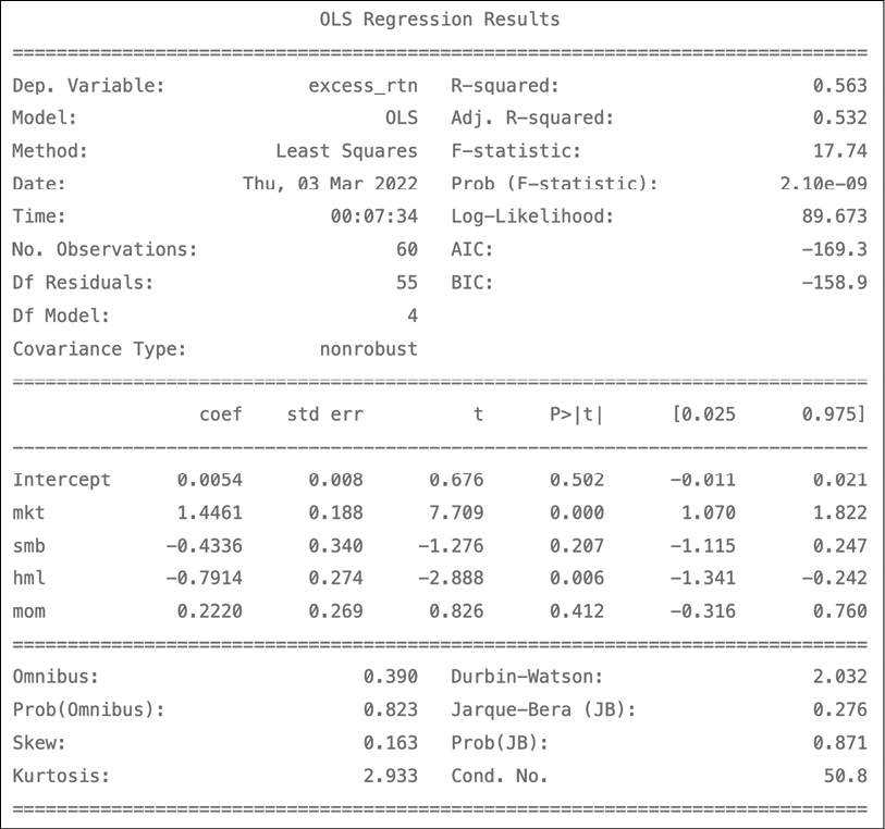
Figure 8.7: The summary of the estimated four-factor model
- Estimate the five-factor model:
five_factor_model = smf.ols(
    formula="excess_rtn ~ mkt + smb + hml + rmw + cma",
    data=factor_5_df
).fit()
print(five_factor_model.summary())
Figure 8.8 shows the results:

Figure 8.8: The summary of the estimated five-factor model
According to the five-factor model, Amazon’s excess returns are negatively exposed to most of the factors (all but the market factor). Here, we present an example of the interpretation of the coefficients: an increase by 1 percentage point in the market factor results in an increase of 0.015 p.p. In other words, for a 1% return by the market factor, we can expect our portfolio (Amazon’s stock) to return 1.5117 * 1% in excess of the risk-free rate.
Similar to the three-factor model, if the five-factor model fully explains the excess stock returns, the estimated intercept should be statistically indistinguishable from zero (which is the case for the considered problem).
How it works...
In Step 2, we defined the parameters—the ticker of the considered stock and timeframes.
In Step 3, we downloaded the necessary datasets using pandas_datareader, which provides us with a convenient way of downloading the risk factor-related data without manually downloading the CSV files. For more information on this process, please refer to the Estimating the Fama-French three-factor model recipe.
In Steps 4 and 5, we downloaded Amazon’s stock prices and calculated the monthly returns using the previously explained methodology.
In Steps 6 and 7, we joined all the datasets, renamed the columns, and calculated the excess returns. When using the join method without specifying what we want to join on (the on argument), the default is the index of the DataFrames.
This way, we prepared all the necessary inputs for the four- and five-factor models. We also had to divide all the data we downloaded from Prof. French’s website by 100 to arrive at the correct scale.
SMB factor in the five-factor dataset is calculated differently compared to how it is in the three-factor dataset. For more details, please refer to the link in the See also section of this recipe.
In Step 8 and Step 9, we estimated the models using the functional form of OLS regression from the statsmodels library. The functional form automatically adds the intercept to the regression equation.
See also
For details on the calculation of the factors, please refer to the following links:
- Momentum factor: https://mba.tuck.dartmouth.edu/pages/faculty/ken.french/Data_Library/det_mom_factor.html
- Five-factor model: https://mba.tuck.dartmouth.edu/pages/faculty/ken.french/Data_Library/f-f_5_factors_2x3.html
For papers introducing the four- and five-factor models, please refer to the following links:
- Carhart, M. M. (1997), “On Persistence in Mutual Fund Performance,” The Journal of Finance, 52, 1 (1997): 57-82
- Fama, E. F. and French, K. R. 2015. “A five-factor asset pricing model,” Journal of Financial Economics, 116(1): 1-22: https://doi.org/10.1016/j.jfineco.2014.10.010
Estimating cross-sectional factor models using the Fama-MacBeth regression
In the previous recipes, we have covered estimating different factor models using a single asset or portfolio as the dependent variable. However, we can estimate the factor models for multiple assets at once, using cross-section (panel) data.
Following this approach, we can:
- Estimate the portfolios’ exposure to the risk factors and learn how much those factors drive the portfolios’ returns
- Understand how much taking a given risk is worth by knowing the premium that the market pays for the exposure to a certain factor
Knowing the risk premiums, we can then estimate the returns for any portfolio provided we can approximate that portfolio’s exposure to the risk factors.
While estimating cross-sectional regression, we can encounter multiple problems due to the fact that some assumptions of linear regression might not hold. We might encounter the following:
- Heteroskedasticity and serial correlation, leading to the covariation of residuals
- Multicollinearity
- Measurement errors
To solve those issues, we can use a technique called the Fama-MacBeth regression, which is a two-step procedure specifically designed to estimate the premiums rewarded by the market for the exposure to certain risk factors.
The steps are as follows:
- Obtain the factor loadings by estimating N (the number of portfolios/assets) time-series regressions of excess returns on the factors:
![]()
- Obtain the risk premiums by estimating T (the number of periods) cross-sectional regressions, one for each period:
![]()
In this recipe, we estimate the Fama-MacBeth regression using five risk factors and the returns of 12 industry portfolios, also available on Prof. French’s website.
How to do it…
Execute the following steps to estimate the Fama-MacBeth regression:
- Import the libraries:
import pandas as pd import pandas_datareader.data as web from linearmodels.asset_pricing import LinearFactorModel - Specify the time horizon:
START_DATE = "2010" END_DATE = "2020-12" - Download and adjust the risk factors from Prof. French’s website:
factor_5_df = ( web.DataReader("F-F_Research_Data_5_Factors_2x3", "famafrench", start=START_DATE, end=END_DATE)[0] .div(100) ) - Download and adjust the returns of 12 Industry Portfolios from Prof. French’s website:
portfolio_df = ( web.DataReader("12_Industry_Portfolios", "famafrench", start=START_DATE, end=END_DATE)[0] .div(100) .sub(factor_5_df["RF"], axis=0) ) - Drop the risk-free rate from the factor dataset:
factor_5_df = factor_5_df.drop("RF", axis=1) - Estimate the Fama-MacBeth regression and print the summary:
five_factor_model = LinearFactorModel(
    portfolios=portfolio_df,
    factors=factor_5_df
)
result = five_factor_model.fit()
print(result)
Running the snippet generates the following summary:

Figure 8.9: The results of the Fama-MacBeth regression
The results in the table are average risk premiums from the T cross-sectional regressions.
We can also print the full summary (containing the risk premiums and each portfolio’s factor loadings). To do so, we need to run the following line of code:
print(result.full_summary)
How it works…
In the first two steps, we imported the required libraries and defined the start and end date of our exercise. In total, we will be using 11 years of monthly data, resulting in 132 observations of the variables (denoted as T ). For the end date, we had to specify 2020-12. Using 2020 alone would result in the downloaded datasets ending with January 2020.
In Step 3, we downloaded the five-factor data set using pandas_datareader. We adjusted the values to express percentages by dividing them by 100.
In Step 4, we downloaded the returns on 12 Industry Portfolios from Prof. French’s website (please see the link in the See also section for more details on the dataset). We have also adjusted the values by dividing them by 100 and calculated the excess returns by subtracting the risk-free rate (available at the factor dataset) from each column of the portfolio dataset. We could do that easily using the sub method as the time periods are an exact match.
In Step 5, we dropped the risk-free rate, as we will not be using it anymore and it will be easier to estimate the Fama-MacBeth regression model with no redundant columns in the DataFrames.
In the last step, we instantiated an object of the LinearFactorModel class and provided both datasets as arguments. Then, we used the fit method to estimate the model. Lastly, we printed the summary.
You might notice a small difference between linearmodels and scikit-learn. In the latter, we provide the data while calling the fit method. With linearmodels, we had to provide the data while creating an instance of the LinearFactorModel class.
In linearmodels, you can also use the formula notation (as we have done when estimating the factor models using statsmodels). To do so, we need to use the from_formula method. An example could look as follows: LinearFactorModel.from_formula(formula, data), where formula is the string containing the formula and data is an object containing both the portfolios/assets and the factors.
There’s more…
We have already estimated the Fama-MacBeth regression using the linearmodels library. However, it might strengthen our understanding of the procedure to carry out the two steps manually.
Execute the following steps to carry out the two steps of the Fama-MacBeth procedure separately:
- Import the libraries:
from statsmodels.api import OLS, add_constant - For the first step of the Fama-MacBeth regression, estimate the factor loadings:
factor_loadings = [] for portfolio in portfolio_df: reg_1 = OLS( endog=portfolio_df.loc[:, portfolio], exog=add_constant(factor_5_df) ).fit() factor_loadings.append(reg_1.params.drop("const")) - Store the factor loadings in a DataFrame:
factor_load_df = pd.DataFrame(
    factor_loadings,
    columns=factor_5_df.columns,
    index=portfolio_df.columns
)
factor_load_df.head()
Running the code generates the following table containing the factor loadings:

Figure 8.10: First step of the Fama-MacBeth regression—the estimated factor loadings
We can compare those numbers to the output of the full summary from the
linearmodelslibrary.
- For the second step of the Fama-MacBeth regression, estimate the risk premiums:
risk_premia = [] for period in portfolio_df.index: reg_2 = OLS( endog=portfolio_df.loc[period, factor_load_df.index], exog=factor_load_df ).fit() risk_premia.append(reg_2.params) - Store the risk premiums in a DataFrame:
risk_premia_df = pd.DataFrame(
    risk_premia,
    index=portfolio_df.index,
    columns=factor_load_df.columns.tolist())
risk_premia_df.head()
Running the code generates the following table containing the risk premiums over time:

Figure 8.11: Second step of the Fama-MacBeth regression—the estimated risk premiums over time
- Calculate the average risk premiums:
risk_premia_df.mean()Running the snippet returns:
Mkt-RF    0.012341
SMB      -0.006291
HML      -0.008927
RMW      -0.000908
CMA      -0.002484
The risk premiums calculated above match the ones obtained from the linearmodels library.
See also
- Documentation of the
linearmodelslibrary can be a good resource for learning about panel regression models (and not only that—it also contains utilities for instrumental variables models and so on) and their implementation in Python: https://bashtage.github.io/linearmodels/index.html - Description of the 12 Industry Portfolios dataset: https://mba.tuck.dartmouth.edu/pages/faculty/ken.french/data_library/det_12_ind_port.html
Further reading about the Fama-MacBeth procedure:
- Fama, E. F., and MacBeth, J. D., “Risk, return, and equilibrium: Empirical tests,” Journal of Political Economy, 81, 3 (1973): 607-636
- Fama, E. F., “Market efficiency, long-term returns, and behavioral finance,” Journal of Financial Economics, 49, 3 (1998): 283-306
Summary
In this chapter, we have constructed some of the most popular factor models. We have started with the simplest one-factor model (the CAPM) and then explained how to approach more advanced three-, four-, and five-factor models. We have also described how we can use the Fama-MacBeth regression to estimate the factor models for multiple assets with appropriate cross-section (panel) data.