
Chapter 2: Examining Bivariate and Multivariate Relationships between Features and Targets
In this chapter, we'll look at the correlation between possible features and target variables. Bivariate exploratory analysis, using crosstabs (two-way frequencies), correlations, scatter plots, and grouped boxplots can uncover key issues for modeling. Common issues include high correlation between features and non-linear relationships between features and the target variable. We will use pandas methods for bivariate analysis and Matplotlib for visualizations in this chapter. We will also discuss the implications of what we find in terms of feature engineering and modeling.
We will also use multivariate techniques to understand the relationship between features. This includes leaning on some machine learning algorithms to identify possibly problematic observations. After, we will provide tentative recommendations for eliminating certain observations from our modeling, as well as for transforming key features.
In this chapter, we will cover the following topics:
- Identifying outliers and extreme values in bivariate relationships
- Using scatter plots to view bivariate relationships between continuous features
- Using grouped boxplots to view bivariate relationships between continuous and categorical features
- Using linear regression to identify data points with significant influence
- Using K-nearest neighbors to find outliers
- Using Isolation Forest to find outliers
Technical requirements
This chapter will rely heavily on the pandas and Matplotlib libraries, but you don't require any prior knowledge of these. If you have installed Python from a scientific distribution, such as Anaconda or WinPython, then these libraries have probably already been installed. We will also be using Seaborn for some of our graphics and the statsmodels library for some summary statistics. If you need to install any of the packages, you can do so by running pip install [package name] from a terminal window or Windows PowerShell. The code for this chapter can be found in this book's GitHub repository at https://github.com/PacktPublishing/Data-Cleaning-and-Exploration-with-Machine-Learning.
Identifying outliers and extreme values in bivariate relationships
It is hard to develop a reliable model without having a good sense of the bivariate relationships in our data. We not only care about the relationship between particular features and target variables but also about how features move together. If features are highly correlated, then modeling their independent effect becomes tricky or unnecessary. This may be a challenge, even if the features are highly correlated over just a range of values.
Having a good understanding of bivariate relationships is also important for identifying outliers. A value might be unexpected, even if it is not an extreme value. This is because some values for a feature are unusual when a second feature has certain values. This is easy to illustrate when one feature is categorical and the other is continuous.
The following diagram illustrates the number of bird sightings per day over several years but shows different distributions for the two sites. One site has a (mean) sightings per day of 33, while the other has 52. (This is a fictional example that's been pulled from my Python Data Cleaning Cookbook.) The overall mean (not shown) is 42. What should we make of a value of 58 for daily sightings? Is it an outlier? This depends on which of the two sites was being observed. If there were 58 sightings in a day at site A, 58 would be an unusually high number. However, this wouldn't be true for site B, where 58 sightings would not be very different from the mean for that site:
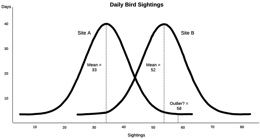
Figure 2.1 – Daily Bird Sightings
This hints at a useful rule of thumb: whenever a feature of interest is correlated with another feature, we should take that relationship into account when we're trying to identify outliers (or any modeling with that feature, actually). It is helpful to state this a little more precisely and extend it to cases where both features are continuous. If we assume a linear relationship between feature x and feature y, we can describe that relationship with the familiar y = mx + b equation, where m is the slope and b is the y-intercept. Then, we can expect the value of y to be somewhere close to x times the estimated slope, plus the y-intercept. Unexpected values are those that deviate substantially from this relationship, where the value of y is much higher or lower than what would be predicted, given the value of x. This can be extended to multiple x, or predictor, variables.
In this section, we will learn how to identify outliers and unexpected values by examining the relationship a feature has with another feature. In subsequent sections of this chapter, we will use multivariate techniques to make additional improvements to our outlier detection.
We will work with data based on COVID-19 cases by country in this section. The dataset contains cases and deaths per million people in the population. We will treat both columns as possible targets. It also contains demographic data for each country, such as GDP per capita, median age, and diabetes prevalence. Let's get started:
Note
Our World in Data provides COVID-19 public-use data at https://ourworldindata.org/coronavirus-source-data. The dataset that's being used in this section was downloaded on July 9, 2021. There are more columns in the data than I have included. I created the region column based on country.
- Let's start by loading the COVID-19 dataset and looking at how it is structured. We will also import the Matplotlib and Seaborn libraries since we will do a couple of visualizations:
import pandas as pd
import matplotlib.pyplot as plt
import seaborn as sns
covidtotals = pd.read_csv("data/covidtotals.csv")
covidtotals.set_index("iso_code", inplace=True)
covidtotals.info()
<class 'pandas.core.frame.DataFrame'>
Index: 221 entries, AFG to ZWE
Data columns (total 16 columns):
# Column Non-Null Count Dtype
-- -------- --------------- -------
0 lastdate 221 non-null object
1 location 221 non-null object
2 total_cases 192 non-null float64
3 total_deaths 185 non-null float64
4 total_cases_mill 192 non-null float64
5 total_deaths_mill 185 non-null float64
6 population 221 non-null float64
7 population_density 206 non-null float64
8 median_age 190 non-null float64
9 gdp_per_capita 193 non-null float64
10 aged_65_older 188 non-null float64
11 total_tests_thous 13 non-null float64
12 life_expectancy 217 non-null float64
13 hospital_beds_thous 170 non-null float64
14 diabetes_prevalence 200 non-null float64
15 region 221 non-null object
dtypes: float64(13), object(3)
memory usage: 29.4+ KB
- A great place to start with our examination of bivariate relationships is with correlations. First, let's create a DataFrame that contains a few key features:
totvars = ['location','total_cases_mill',
'total_deaths_mill']
demovars = ['population_density','aged_65_older',
'gdp_per_capita','life_expectancy',
'diabetes_prevalence']
covidkeys = covidtotals.loc[:, totvars + demovars]
- Now, we can get the Pearson correlation matrix for these features. There is a strong positive correlation of 0.71 between cases and deaths per million. The percentage of the population that's aged 65 or older is positively correlated with cases and deaths, at 0.53 for both. Life expectancy is also highly correlated with cases per million. There seems to be at least some correlation of gross domestic product (GDP) per person with cases:
corrmatrix = covidkeys.corr(method="pearson")
corrmatrix
total_cases_mill total_deaths_mill
total_cases_mill 1.00 0.71
total_deaths_mill 0.71 1.00
population_density 0.04 -0.03
aged_65_older 0.53 0.53
gdp_per_capita 0.46 0.22
life_expectancy 0.57 0.46
diabetes_prevalence 0.02 -0.01
population_density aged_65_older gdp_per_capita
total_cases_mill 0.04 0.53 0.46
total_deaths_mill -0.03 0.53 0.22
population_density 1.00 0.06 0.41
aged_65_older 0.06 1.00 0.49
gdp_per_capita 0.41 0.49 1.00
life_expectancy 0.23 0.73 0.68
diabetes_prevalence 0.01 -0.06 0.12
life_expectancy diabetes_prevalence
total_cases_mill 0.57 0.02
total_deaths_mill 0.46 -0.01
population_density 0.23 0.01
aged_65_older 0.73 -0.06
gdp_per_capita 0.68 0.12
life_expectancy 1.00 0.19
diabetes_prevalence 0.19 1.00
It is worth noting the correlation between possible features, such as between life expectancy and GDP per capita (0.68) and life expectancy and those aged 65 or older (0.73).
- It can be helpful to see the correlation matrix as a heat map. This can be done by passing the correlation matrix to the Seaborn heatmap method:
sns.heatmap(corrmatrix, xticklabels =
corrmatrix.columns, yticklabels=corrmatrix.columns,
cmap="coolwarm")
plt.title('Heat Map of Correlation Matrix')
plt.tight_layout()
plt.show()
This creates the following plot:

Figure 2.2 – Heat map of COVID data, with the strongest correlations in red and peach
We want to pay attention to the cells shown with warmer colors – in this case, mainly peach. I find that using a heat map helps me keep correlations in mind when modeling.
Note
All the color images contained in this book can be downloaded. Check the Preface of this book for the respective link.
- Let's take a closer look at the relationship between total cases per million and deaths per million. One way to get a better sense of this than with just a correlation coefficient is by comparing the high and low values for each and seeing how they move together. In the following code, we're using the qcut method to create a categorical feature with five values distributed relatively evenly, from very low to very high, for cases. We have done the same for deaths:
covidkeys['total_cases_q'] =
pd.qcut(covidkeys['total_cases_mill'],
labels=['very low','low','medium','high',
'very high'], q=5, precision=0)
covidkeys['total_deaths_q'] =
pd.qcut(covidkeys['total_deaths_mill'],
labels=['very low','low','medium','high',
'very high'], q=5, precision=0)
- We can use the crosstab function to view the number of countries for each quintile of cases and quintile of deaths. As we would expect, most of the countries are along the diagonal. There are 27 countries with very low cases and very low deaths, and 25 countries with very high cases and very high deaths. The interesting counts are those not on the diagonal, such as the four countries with very high cases but only medium deaths, nor the one with medium cases and very high deaths. Let's also look at the means of our features so that we can reference them later:
pd.crosstab(covidkeys.total_cases_q,
covidkeys.total_deaths_q)
total_deaths_q very low low medium high very high
total_cases_q
very low 27 7 0 0 0
low 9 24 4 0 0
medium 1 6 23 6 1
high 0 0 6 21 11
very high 0 0 4 10 25
covidkeys.mean()
total_cases_mill 36,649
total_deaths_mill 683
population_density 453
aged_65_older 9
gdp_per_capita 19,141
life_expectancy 73
diabetes_prevalence 8
- Let's take a closer look at the countries away from the diagonal. Four countries – Cyprus, Kuwait, Maldives, and Qatar – have fewer deaths per million than average but well above average cases per million. Interestingly, all four countries are very small in terms of population; three of the four have population densities far below the average of 453; again, three of the four have people aged 65 or older percentages that are much lower than average:
covidtotals.loc[(covidkeys.total_cases_q=="very high")
& (covidkeys.total_deaths_q=="medium")].T
iso_code CYP KWT MDV QAT
lastdate 2021-07-07 2021-07-07 2021-07-07 2021-07-07
location Cyprus Kuwait Maldives Qatar
total_cases 80,588 369,227 74,724 222,918
total_deaths 380 2,059 213 596
total_cases_mill 90,752 86,459 138,239 77,374
total_deaths_mill 428 482 394 207
population 888,005 4,270,563 540,542 2,881,060
population_density 128 232 1,454 227
median_age 37 34 31 32
gdp_per_capita 32,415 65,531 15,184 116,936
aged_65_older 13 2 4 1
total_tests_thous NaN NaN NaN NaN
life_expectancy 81 75 79 80
hospital_beds_thous 3 2 NaN 1
diabetes_prevalence 9 16 9 17
region Eastern West South West
Europe Asia Asia Asia
- Let's take a closer look at the country with more deaths than we would have expected based on cases. For Mexico, the number of cases per million are well below average, while the number of deaths per million are quite a bit above average:
covidtotals.loc[(covidkeys. total_cases_q=="medium")
& (covidkeys.total_deaths_q=="very high")].T
iso_code MEX
lastdate 2021-07-07
location Mexico
total_cases 2,558,369
total_deaths 234,192
total_cases_mill 19,843
total_deaths_mill 1,816
population 128,932,753
population_density 66
median_age 29
gdp_per_capita 17,336
aged_65_older 7
total_tests_thous NaN
life_expectancy 75
hospital_beds_thous 1
diabetes_prevalence 13
region North America
Correlation coefficients and heat maps are a good place to start when we want to get a sense of the bivariate relationships in our dataset. However, it can be hard to visualize the relationship between continuous variables with just a correlation coefficient. This is particularly true when the relationship is not linear – that is, when it varies based on the ranges of a feature. We can often improve our understanding of the relationship between two features with a scatter plot. We will do that in the next section.
Using scatter plots to view bivariate relationships between continuous features
In this section, we'll learn how to get a scatter plot of our data.
We can use scatter plots to get a more complete picture of the relationship between two features than what can be detected by a correlation coefficient alone. This is particularly useful when that relationship changes across certain ranges of the data. In this section, we will create scatter plots of some of the same features we examined in the previous section. Let's get started:
- It is helpful to plot a regression line through the data points. We can do this with Seaborn's regplot method. Let's load the COVID-19 data again, along with the Matplotlib and Seaborn libraries, and generate a scatter plot of total_cases_mill by total_deaths_mill:
import pandas as pd
import numpy as np
import matplotlib.pyplot as plt
import seaborn as sns
covidtotals = pd.read_csv("data/covidtotals.csv")
covidtotals.set_index("iso_code", inplace=True)
ax = sns.regplot(x="total_cases_mill",
y="total_deaths_mill", data=covidtotals)
ax.set(xlabel="Cases Per Million", ylabel="Deaths Per
Million", title="Total COVID Cases and Deaths by
Country")
plt.show()
This produces the following plot:
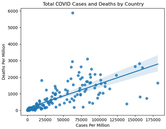
Figure 2.3 – Total COVID Cases and Deaths by Country
The regression line is an estimate of the relationship between cases per million and deaths per million. The slope of the line indicates how much we can expect deaths per million to increase with a 1-unit increase in cases per million. Those points on the scatter plot that are significantly above the regression line should be examined more closely.
- The country with deaths per million near 6,000 and cases per million below 75,000 is clearly an outlier. Let's take a closer look:
covidtotals.loc[(covidtotals.total_cases_mill<75000)
& (covidtotals.total_deaths_mill>5500)].T
iso_code PER
lastdate 2021-07-07
location Peru
total_cases 2,071,637
total_deaths 193,743
total_cases_mill 62,830
total_deaths_mill 5,876
population 32,971,846
population_density 25
median_age 29
gdp_per_capita 12,237
aged_65_older 7
total_tests_thous NaN
life_expectancy 77
hospital_beds_thous 2
diabetes_prevalence 6
region South America
Here, we can see that the outlier country is Peru. Peru does have above-average cases per million, but its number of deaths per million is still much greater than would be expected given the number of cases. If we draw a line that's perpendicular to the x axis at 62,830, we can see that it crosses the regression line at about 1,000 deaths per million, which is far fewer than the 5,876 for Peru. The only other values in the data for Peru that also stand out as very different from the dataset averages are population density and GDP per person, both of which are substantially lower than average. Here, none of our features may help us explain the high number of deaths in Peru.
Note
When creating a scatter plot, it is common to put a feature or predictor variable on the x axis and a target variable on the y axis. If a regression line is drawn, then that represents the increase in the target that's been predicted by a 1-unit increase in the predictor. But scatter plots can also be used to examine the relationship between two predictors or two possible targets.
Looking back at how we defined an outlier in Chapter 1, Examining the Distribution of Features and Targets, an argument can be made that Peru is an outlier. But we still have more work to do before we can come to that conclusion. Peru is not the only country with points on the scatter plot far above or below the regression line. It is generally a good idea to investigate many of these points. Let's take a look:
- Creating scatter plots that contain most of the key continuous features can help us identify other possible outliers and better visualize the correlations we observed in the first section of this chapter. Let's create scatter plots of people who are aged 65 and older and GDP per capita with total cases per million:
fig, axes = plt.subplots(1,2, sharey=True)
sns.regplot(x=covidtotals.aged_65_older,
y=covidtotals.total_cases_mill, ax=axes[0])
sns.regplot(x=covidtotals.gdp_per_capita,
y=covidtotals.total_cases_mill, ax=axes[1])
axes[0].set_xlabel("Aged 65 or Older")
axes[0].set_ylabel("Cases Per Million")
axes[1].set_xlabel("GDP Per Capita")
axes[1].set_ylabel("")
plt.suptitle("Age 65 Plus and GDP with Cases Per
Million")
plt.tight_layout()
fig.subplots_adjust(top=0.92)
plt.show()
This produces the following plot:
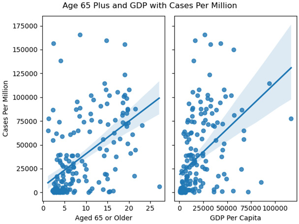
Figure 2.4 – Age 65 Plus and GDP with Cases Per Million
These scatter plots show that some countries that had very high cases per million had values close to what we would expect, given the age of the population or the GDP. These are extreme values, but not necessarily outliers as we have defined them.
It is possible to use scatter plots to illustrate the relationships between two features and a target, all in one graphic. Let's return to the land temperatures data that we worked with in the previous chapter to explore this.
Data Note
The land temperature dataset contains the average temperature readings (in Celsius) in 2019 from over 12,000 stations across the world, though the majority of the stations are in the United States. The dataset was retrieved from the Global Historical Climatology Network integrated database. It has been made available for public use by the United States National Oceanic and Atmospheric Administration at https://www.ncdc.noaa.gov/data-access/land-based-station-data/land-based-datasets/global-historical-climatology-network-monthly-version-4.
- We expect the average temperature at a weather station to be impacted by both latitude and elevation. Let's say that our previous analysis showed that elevation does not start having much of an impact on temperature until approximately the 1,000-meter mark. We can split the landtemps DataFrame into low- and high-elevation stations, with 1,000 meters as the threshold. In the following code, we can see that this gives us 9,538 low-elevation stations with an average temperature of 12.16 degrees Celsius, and 2,557 high-elevation stations with an average temperature of 7.58:
landtemps = pd.read_csv("data/landtemps2019avgs.csv")
low, high = landtemps.loc[landtemps.elevation<=1000],
landtemps.loc[landtemps.elevation>1000]
low.shape[0], low.avgtemp.mean()
(9538, 12.161417937651676)
high.shape[0], high.avgtemp.mean()
(2557, 7.58321486951755)
- Now, we can visualize the relationship between elevation and latitude and temperature in one scatter plot:
plt.scatter(x="latabs", y="avgtemp", c="blue",
data=low)
plt.scatter(x="latabs", y="avgtemp", c="red",
data=high)
plt.legend(('low elevation', 'high elevation'))
plt.xlabel("Latitude (N or S)")
plt.ylabel("Average Temperature (Celsius)")
plt.title("Latitude and Average Temperature in 2019")
plt.show()
This produces the following scatter plot:
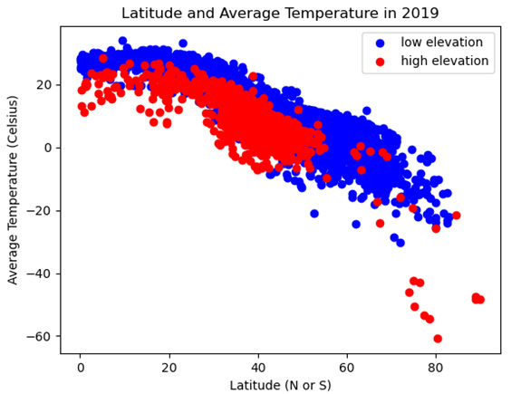
Figure 2.5 – Latitude and Average Temperature in 2019
Here, we can see that the temperatures gradually decrease as the distance from the equator (measured in latitude) increases. We can also see that high-elevation weather stations (those with red dots) are generally below low-elevation stations – that is, they have lower temperatures at similar latitudes.
- There also seems to be at least some difference in slope between high- and low-elevation stations. Temperatures appear to decline more quickly as latitude increases with high-elevation stations. We can draw two regression lines through the scatter plot – one for high and one for low-elevation stations – to get a clearer picture of this. To simplify the code a bit, let's create a categorical feature, elevation_group, for low- and high-elevation stations:
landtemps['elevation_group'] =
np.where(landtemps.elevation<=1000,'low','high')
sns.lmplot(x="latabs", y="avgtemp",
hue="elevation_group", palette=dict(low="blue",
high="red"), legend_out=False, data=landtemps)
plt.xlabel("Latitude (N or S)")
plt.ylabel("Average Temperature")
plt.legend(('low elevation', 'high elevation'),
loc='lower left')
plt.yticks(np.arange(-60, 40, step=20))
plt.title("Latitude and Average Temperature in 2019")
plt.tight_layout()
plt.show()
This produces the following plot:
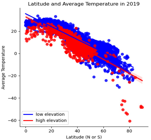
Figure 2.6 – Latitude and Average Temperature in 2019 with regression lines
Here, we can see the steeper negative slope for high-elevation stations.
- If we want to see a scatter plot with two continuous features and a continuous target, rather than forcing one of the features to be dichotomous, as we did in the previous example, we can take advantage of Matplotlib's 3D functionality:
fig = plt.figure()
plt.suptitle("Latitude, Temperature, and Elevation in
2019")
ax = plt.axes(projection='3d')
ax.set_xlabel("Elevation")
ax.set_ylabel("Latitude")
ax.set_zlabel("Avg Temp")
ax.scatter3D(landtemps.elevation, landtemps.latabs,
landtemps.avgtemp)
plt.show()
This produces the following three-dimensional scatter plot:
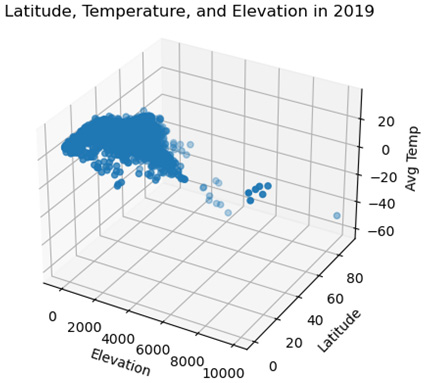
Figure 2.7 – Latitude, Temperature, and Elevation in 2019
Scatter plots are a go-to visualization for teasing out relationships between continuous features. We get a better sense of those relationships than correlation coefficients alone can reveal. However, we need a very different visualization if we are examining the relationship between a continuous feature and a categorical one. Grouped boxplots are useful in those cases. We will learn how to create grouped boxplots with Matplotlib in the next section.
Using grouped boxplots to view bivariate relationships between continuous and categorical features
Grouped boxplots are an underappreciated visualization. They are helpful when we're examining the relationship between continuous and categorical features since they show how the distribution of a continuous feature can vary by the values of the categorical feature.
We can explore this by returning to the National Longitudinal Survey (NLS) data we worked with in the previous chapter. The NLS has one observation per survey respondent but collects annual data on education and employment (data for each year is captured in different columns).
Data Note
As stated in Chapter 1, Examining the Distribution of Features and Targets, the NLS of Youth is conducted by the United States Bureau of Labor Statistics. Separate files for SPSS, Stata, and SAS can be downloaded from the respective repository. The NLS data can be downloaded from https://www.nlsinfo.org/investigator/pages/search.
Follow these steps to create grouped bloxplots:
- Among the many columns in the NLS DataFrame, there's highestdegree and weeksworked17, which represent the highest degree the respondent earned and the number of weeks the person worked in 2017, respectively. Let's look at the distribution of weeks worked for each value of the degree that was earned. First, we must define a function, gettots, to get the descriptive statistics we want. Then, we must pass a groupby series object, groupby(['highestdegree'])['weeksworked17'], to that function using apply:
Note
We will not go over how to use groupby or apply in this book. I have covered many examples of their use in my book, Python Data Cleaning Cookbook.
nls97 = pd.read_csv("data/nls97.csv")
nls97.set_index("personid", inplace=True)
def gettots(x):
out = {}
out['min'] = x.min()
out['qr1'] = x.quantile(0.25)
out['med'] = x.median()
out['qr3'] = x.quantile(0.75)
out['max'] = x.max()
out['count'] = x.count()
return pd.Series(out)
nls97.groupby(['highestdegree'])['weeksworked17'].
apply(gettots).unstack()
min qr1 med qr3 max count
highestdegree
0. None 0 0 40 52 52 510
1. GED 0 8 47 52 52 848
2. High School 0 31 49 52 52 2,665
3. Associates 0 42 49 52 52 593
4. Bachelors 0 45 50 52 52 1,342
5. Masters 0 46 50 52 52 538
6. PhD 0 46 50 52 52 51
7. Professional 0 47 50 52 52 97
Here, we can see how different the distribution of weeks worked for people with less than a high school degree is from that distribution for people with a bachelor's degree or more. For those with no degree, more than 25% had 0 weeks worked. For those with a bachelor's degree, even those at the 25th percentile worked 45 weeks during the year. The interquartile range covers the whole distribution for individuals with no degree (0 to 52), but only a small part of the range for individuals with bachelor's degrees (45 to 52).
We should also make note of the class imbalance for highestdegree. The counts get quite small after master's degrees and the counts for high school degrees are nearly twice that of the next largest group. We will likely need to collapse some categories before we do any modeling with this data.
- Grouped boxplots make the differences in distributions even clearer. Let's create some with the same data. We will use Seaborn for this plot:
import seaborn as sns
myplt = sns.boxplot(x='highestdegree',
y= 'weeksworked17' , data=nls97,
order=sorted(nls97.highestdegree.dropna().unique()))
myplt.set_title("Boxplots of Weeks Worked by Highest
Degree")
myplt.set_xlabel('Highest Degree Attained')
myplt.set_ylabel('Weeks Worked 2017')
myplt.set_xticklabels(myplt.get_xticklabels(),
rotation=60, horizontalalignment='right')
plt.tight_layout()
plt.show()
This produces the following plot:
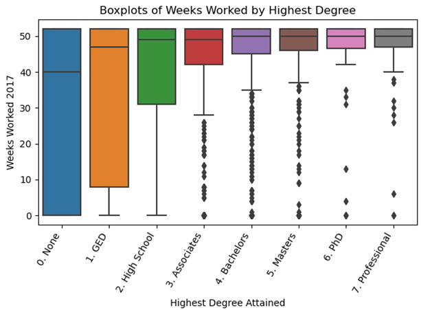
Figure 2.8 – Boxplots of Weeks Worked by Highest Degree
The grouped boxplots illustrate the dramatic difference in interquartile range for weeks worked by the degree earned. At the associate's degree level (a 2-year college degree in the United States) or above, there are values below the whiskers, represented by dots. Below the associate's degree level, the boxplots do not identify any outliers or extreme values. For example, a 0 weeks worked value is not an extreme value for someone with no degree, but it is for someone with an associate's degree or more.
- We can also use grouped boxplots to illustrate how the distribution of COVID-19 cases varies by region. Let's also add a swarmplot to view the data points since there aren't too many of them:
sns.boxplot(x='total_cases_mill', y='region',
data=covidtotals)
sns.swarmplot(y="region", x="total_cases_mill",
data=covidtotals, size=1.5, color=".3", linewidth=0)
plt.title("Boxplots of Total Cases Per Million by
Region")
plt.xlabel("Cases Per Million")
plt.ylabel("Region")
plt.tight_layout()
plt.show()
This produces the following plot:
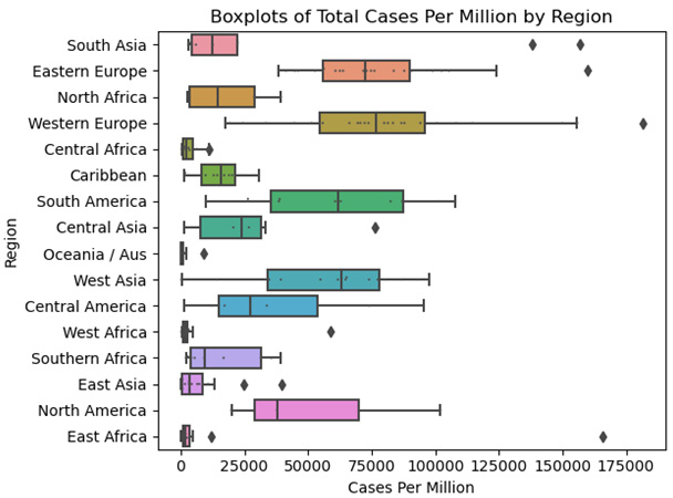
Figure 2.9 – Boxplots of Total Cases Per Million by Region
These grouped boxplots show just how much the median cases per million varies by region, from East Africa and East Asia on the low end to Eastern Europe and Western Europe on the high end. Extremely high values for East Asia are below the first quartile for Western Europe. We should probably avoid drawing too many conclusions beyond that since the counts for most regions (the number of countries) are fairly small.
So far in this chapter, we have focused mainly on bivariate relationships between features, as well as those between a feature and a target. The statistics and visualizations we have generated will inform the modeling we will do. We are already getting a sense of likely features, their influence on targets, and how the distributions of some features change with the values of another feature.
We will explore multivariate relationships in the remaining sections of this chapter. We want to have some sense of how multiple features move together before we begin our modeling. Do some features no longer matter once other features are included? Which observations pull on our parameter estimates more than others, and what are the implications for model fitting? Similarly, which observations are not like the others, because they either have invalid values or because they seem to be capturing a completely different phenomenon than the other observations? We will begin to answer those questions in the next three sections. Although we will not get any definitive answers until we construct our models, we can start making difficult modeling decisions by anticipating them.
Using linear regression to identify data points with significant influence
It is not unusual to find that a few observations have a surprisingly high degree of influence on our model, our parameter estimates, and our predictions. This may or may not be desirable. Observations with significant influence may be unhelpful if they reflect a different social or natural process than the rest of the data does. For example, let's say we have a dataset of flying animals that migrate a great distance, and this is almost exclusively bird species, except for data on monarch butterflies. If we are using the wing architecture as a predictor of migration distance, the monarch butterfly data should probably be removed.
We should return to the distinction we made in the first section between an extreme value and an outlier. We mentioned that an outlier can be thought of as an observation with feature values, or relationships between feature values, that are so unusual that they cannot help explain relationships in the rest of the data. An extreme value, on the other hand, may reflect a natural and explainable trend in a feature, or the same relationship between features that has been observed throughout the data.
Distinguishing between an outlier and an extreme value matters most with observations that have a high influence on our model. A standard measure of influence in regression analysis is Cook's Distance (Cook's D). This gives us a measure of how much our predictions would change if an observation were to be removed from the data.
Let's construct a relatively straightforward multivariate regression model in this section with the COVID-19 data we have been using, and then generate a Cook's D value for each observation:
- Let's load the COVID-19 data and the Matplotlib and statsmodels libraries:
import pandas as pd
import matplotlib.pyplot as plt
import statsmodels.api as sm
covidtotals = pd.read_csv("data/covidtotals.csv")
covidtotals.set_index("iso_code", inplace=True)
- Now, let's look at the distribution of total cases per million in population and some possible predictors:
xvars = ['population_density','aged_65_older',
'gdp_per_capita','diabetes_prevalence']
covidtotals[['total_cases_mill'] + xvars].
quantile(np.arange(0.0,1.05,0.25))
total_cases_mill population_density aged_65_older
0.00 8.52 0.14 1.14
0.25 2,499.75 36.52 3.50
0.50 19,525.73 87.25 6.22
0.75 64,834.62 213.54 13.92
1.00 181,466.38 20,546.77 27.05
gdp_per_capita diabetes_prevalence
0.00 661.24 0.99
0.25 3,823.19 5.34
0.50 12,236.71 7.20
0.75 27,216.44 10.61
1.00 116,935.60 30.53
- Next, let's define a function, getlm, that uses statsmodels to run a linear regression model and generate influence statistics, including Cook's D. This function takes a DataFrame, the name of the target column, and the column names for the features (it is customary to refer to a target as y and features as X).
We will use dropna to drop any observations where one of the features has a missing value. The function returns the estimated coefficients (along with pvalues), the influence measures for each observation, and the full regression results (lm):
def getlm(df, ycolname, xcolnames):
df = df[[ycolname] + xcolnames].dropna()
y = df[ycolname]
X = df[xcolnames]
X = sm.add_constant(X)
lm = sm.OLS(y, X).fit()
influence = lm.get_influence().summary_frame()
coefficients = pd.DataFrame(zip(['constant'] +
xcolnames, lm.params, lm.pvalues),
columns=['features','params','pvalues'])
return coefficients, influence, lm
- Now, we can call the getlm function while specifying the total cases per million as the target and population density (people per square mile), age 65 plus the percentage, GDP per capita, and diabetes prevalence as predictors. Then, we can print the parameter estimates. Ordinarily, we would want to look at a full summary of the model, which can be generated with lm.summary(). We'll skip that here for ease of understanding:
coefficients, influence, lm = getlm(covidtotals,
'total_cases_mill', xvars)
coefficients
features params pvalues
0 constant -1,076.471 0.870
1 population_density -6.906 0.030
2 aged_65_older 2,713.918 0.000
3 gdp_per_capita 0.532 0.001
4 diabetes_prevalence 736.809 0.241
The coefficients for population density, age 65 plus, and GDP are all significant at the 95% level (have p-values less than 0.05). The result for population density is interesting since our bivariate analysis did not reveal a relationship between population density and cases per million. The coefficient indicates a 6.9-point reduction in cases per million, with a 1-point increase in people per square mile. Put more broadly, more crowded countries have fewer cases per million people once we control for the percentage of people that are 65 or older and their GDP per capita. This could be spurious, or it could be a relationship that can only be detected with multivariate analysis. (It could also be that population density is highly correlated with a feature that has a greater effect on cases per million, but that feature has been left out of the model. This would give us a biased coefficient estimate for population density.)
- We can use the influence DataFrame that we created in our call to getlm to take a closer look at those observations with a high Cook's D. One way of defining a high Cook's D is by using three times the mean value for Cook's D for all observations. Let's create a covidtotalsoutliers DataFrame with all the values above that threshold.
There were 13 countries with Cook's D values above the threshold. Let's print out the first five in descending order of the Cook's D value. Bahrain and Maldives are in the top quarter of the distribution for cases (see the descriptives we printed earlier in this section). They also have high population densities and low percentages of age 65 or older. All else being equal, we would expect lower cases per million for those two countries, given what our model says about the relationship between population density and age to cases. Bahrain does have a very high GDP per capita, however, which our model tells us is associated with high case numbers.
Singapore and Hong Kong have extremely high population densities and below-average cases per million, particularly Hong Kong. These two locations, alone, may account for the direction of the population density coefficient. They both also have very high GDP per capita values, which might be a drag on that coefficient. It may just be that our model should not include locations that are city-states:
influencethreshold = 3*influence.cooks_d.mean()
covidtotals = covidtotals.join(influence[['cooks_d']])
covidtotalsoutliers =
covidtotals.loc[covidtotals.cooks_d >
influencethreshold]
covidtotalsoutliers.shape
(13, 17)
covidtotalsoutliers[['location','total_cases_mill',
'cooks_d'] + xvars].sort_values(['cooks_d'],
ascending=False).head()
location total_cases_mill cooks_d population_density
iso_code
BHR Bahrain 156,793.409 0.230 1,935.907
SGP Singapore 10,709.116 0.200 7,915.731
HKG Hong Kong 1,593.307 0.181 7,039.714
JPN Japan 6,420.871 0.095 347.778
MDV Maldives 138,239.027 0.069 1,454.433
aged_65_older gdp_per_capita diabetes_prevalence
iso_code
BHR 2.372 43,290.705 16.520
SGP 12.922 85,535.383 10.990
HKG 16.303 56,054.920 8.330
JPN 27.049 39,002.223 5.720
MDV 4.120 15,183.616 9.190
- So, let's take a look at our regression model estimates if we remove Hong Kong
and Singapore:
Note
I am not necessarily recommending this as an approach. We should look at each observation more carefully than we have done so far to determine whether it makes sense to exclude it from our analysis. We are removing the observations here just to demonstrate their effect on the model.
coefficients, influence, lm2 =
getlm(covidtotals.drop(['HKG','SGP']),
'total_cases_mill', xvars)
coefficients
features params pvalues
0 constant -2,864.219 0.653
1 population_density 26.989 0.005
2 aged_65_older 2,669.281 0.000
3 gdp_per_capita 0.553 0.000
4 diabetes_prevalence 319.262 0.605
The big change in the model is that the population density coefficient has now changed direction. This demonstrates how sensitive the population density estimate is to outlier observations whose feature and target values may not be generalizable to the rest of the data. In this case, that might be true for city-states such as Hong Kong and Singapore.
Generating influence measures with linear regression is a very useful technique, and it has the advantage that it is fairly easy to interpret, as we have seen. However, it does have one important disadvantage: it assumes a linear relationship between features, and that features are normally distributed. This is often not the case. We also needed to understand the relationships in the data enough to create labels, to identify total cases per million as the target. This is not always possible either. In the next two sections, we'll look at machine learning algorithms for outlier detection that do not make these assumptions.
Using K-nearest neighbors to find outliers
Machine learning tools can help us identify observations that are unlike others when we have unlabeled data – that is, when there is no target or dependent variable. Even when selecting targets and features is relatively straightforward, it might be helpful to identify outliers without making any assumptions about relationships between features, or the distribution of features.
Although we typically use K-nearest neighbors (KNN) with labeled data, for classification or regression problems, we can use it to identify anomalous observations. These are observations where there is the greatest difference between their values and their nearest neighbors' values. KNN is a very popular algorithm because it is intuitive, makes few assumptions about the structure of the data, and is quite flexible. The main disadvantage of KNN is that it is not as efficient as many other approaches, particularly parametric techniques such as linear regression. We will discuss these advantages in much greater detail in Chapter 9, K-Nearest Neighbors, Decision Tree, Random Forest, and Gradient Boosted Regression, and Chapter 12, K-Nearest Neighbors for Classification.
We will use PyOD, short for Python outlier detection, to identify countries in the COVID-19 data that are significantly different from others. PyOD can use several algorithms to identify outliers, including KNN. Let's get started:
- First, we need to import the KNN module from PyOD and StandardScaler from the sklearn preprocessing utility functions. We also load the COVID-19 data:
import pandas as pd
from pyod.models.knn import KNN
from sklearn.preprocessing import StandardScaler
covidtotals = pd.read_csv("data/covidtotals.csv")
covidtotals.set_index("iso_code", inplace=True)
Next, we standardize the data, which is important when we have features with very different ranges, from over 100,000 for total cases per million and GDP per capita to less than 20 for diabetes prevalence and age 65 and older. We can use scikit-learn's standard scaler, which converts each feature value into a z-score, as follows:

Here, ![]() is the value for the ith observation of the jth feature,
is the value for the ith observation of the jth feature, ![]() is the mean for feature
is the mean for feature ![]() , and
, and ![]() is the standard deviation for that feature.
is the standard deviation for that feature.
- We can use the scaler for just the features we will be including in our model, and then drop all observations that are missing values for one or more features:
standardizer = StandardScaler()
analysisvars =['location', 'total_cases_mill',
'total_deaths_mill','population_density',
'diabetes_prevalence', 'aged_65_older',
'gdp_per_capita']
covidanalysis =
covidtotals.loc[:,analysisvars].dropna()
covidanalysisstand =
standardizer.fit_transform(covidanalysis.iloc[:,1:])
- Now, we can run the model and generate predictions and anomaly scores. First, we must set contamination to 0.1 to indicate that we want 10% of observations to be identified as outliers. This is pretty arbitrary but not a bad starting point. After using the fit method to run the KNN algorithm, we get predictions (1 if an outlier, 0 if an inlier) and an anomaly score, which is the basis of the prediction (in this case, the top 10% of anomaly scores will get a prediction of 1):
clf_name = 'KNN'
clf = KNN(contamination=0.1)
clf.fit(covidanalysisstand)
y_pred = clf.labels_
y_scores = clf.decision_scores_
- We can combine the two NumPy arrays with the predictions and anomaly scores – y_pred and y_scores, respectively – and convert them into the columns of a DataFrame. This makes it easier to view the range of anomaly scores and their associated predictions. 18 countries have been identified as outliers (this is a result of setting contamination to 0.1). Outliers have anomaly scores of 1.77 to 9.34, while inliers have scores of 0.11 to 1.74:
pred = pd.DataFrame(zip(y_pred, y_scores),
columns=['outlier','scores'],
index=covidanalysis.index)
pred.outlier.value_counts()
0 156
1 18
pred.groupby(['outlier'])[['scores']].
agg(['min','median','max'])
scores
min median max
outlier
0 0.11 0.84 1.74
1 1.77 2.48 9.34
- Let's take a closer look at the countries with the highest anomaly scores:
covidanalysis = covidanalysis.join(pred).
loc[:,analysisvars + ['scores']].
sort_values(['scores'], ascending=False)
covidanalysis.head(10)
location total_cases_mill total_deaths_mill
iso_code …
SGP Singapore 10,709.12 6.15
HKG Hong Kong 1,593.31 28.28
PER Peru 62,830.48 5,876.01
QAT Qatar 77,373.61 206.87
BHR Bahrain 156,793.41 803.37
LUX Luxembourg 114,617.81 1,308.36
BRN Brunei 608.02 6.86
KWT Kuwait 86,458.62 482.14
MDV Maldives 138,239.03 394.05
ARE United Arab Emirates 65,125.17 186.75
aged_65_older gdp_per_capita scores
iso_code
SGP 12.92 85,535.38 9.34
HKG 16.30 56,054.92 8.03
PER 7.15 12,236.71 4.37
QAT 1.31 116,935.60 4.23
BHR 2.37 43,290.71 3.51
LUX 14.31 94,277.96 2.73
BRN 4.59 71,809.25 2.60
KWT 2.35 65,530.54 2.52
MDV 4.12 15,183.62 2.51
ARE 1.14 67,293.48 2.45
Several of the locations we identified as having high influence in the previous section have high anomaly scores, including Singapore, Hong Kong, Bahrain, and Maldives. This is more evidence that we need to take a closer look at the data for these countries. Perhaps there is invalid data or there are theoretical reasons why they are very different than the rest of the data.
Unlike the linear model in the previous section, there is no defined target. We include both total cases per million and total deaths per million in this case. Peru has been identified as an outlier here, though it was not with the linear model. This is partly because of Peru's very high deaths per million, which is the highest in the dataset (we did not use deaths per million in our linear regression model).
- Notice that Japan is not on this list of outliers. Let's take a look at its anomaly score:
covidanalysis.loc['JPN','scores']
2.03
The anomaly score is the 15th highest in the dataset. Compare this with the 4th highest Cook's D score for Japan from the previous section.
It is interesting to compare these results with a similar analysis we could conduct with Isolation Forest. We will do that in the next section.
Note
This has been a very simplified example of the approach we would take with a typical machine learning project. The most important omission here is that we are conducting our analysis on the full dataset. For reasons we will discuss at the beginning of Chapter 4, Encoding, Transforming, and Scaling Features, we want to split our data into training and testing datasets very early in the process. We will learn how to incorporate outlier detection in a machine learning pipeline in the remaining chapters of this book.
Using Isolation Forest to find outliers
Isolation Forest is a relatively new machine learning technique for identifying anomalies. It has quickly become popular, partly because its algorithm is optimized to find outliers, rather than normal values. It finds outliers by successively partitioning the data until a data point has been isolated. Points that require fewer partitions to be isolated receive higher anomaly scores. This process turns out to be fairly easy on system resources. In this section, we will learn how to use it to detect outlier COVID-19 cases and deaths.
Isolation Forest is a good alternative to KNN, particularly when we're working with large datasets. The efficiency of the algorithm allows it to handle large samples and a high number of features. Let's get started:
- We can do an analysis similar to the one in the previous section with Isolation Forest rather than KNN. Let's start by loading scikit-learn's StandardScaler and IsolationForest modules, as well as the COVID-19 data:
import pandas as pd
import matplotlib.pyplot as plt
from sklearn.preprocessing import StandardScaler
from sklearn.ensemble import IsolationForest
covidtotals = pd.read_csv("data/covidtotals.csv")
covidtotals.set_index("iso_code", inplace=True)
- Next, we must standardize the data:
analysisvars = ['location','total_cases_mill','total_deaths_mill',
'population_density','aged_65_older','gdp_per_capita']
standardizer = StandardScaler()
covidanalysis = covidtotals.loc[:, analysisvars].dropna()
covidanalysisstand =
standardizer.fit_transform(covidanalysis.iloc[:, 1:])
- Now, we are ready to run our anomaly detection model. The n_estimators parameter indicates how many trees to build. Setting max_features to 1.0 will use all of our features. The predict method gives us the anomaly prediction, which is -1 for an anomaly. This is based on the anomaly score, which we can get using decision_function:
clf=IsolationForest(n_estimators=50,
max_samples='auto', contamination=.1,
max_features=1.0)
clf.fit(covidanalysisstand)
covidanalysis['anomaly'] =
clf.predict(covidanalysisstand)
covidanalysis['scores'] =
clf.decision_function(covidanalysisstand)
covidanalysis.anomaly.value_counts()
1 156
-1 18
Name: anomaly, dtype: int64
- Let's take a closer look at the outliers (we will also create a DataFrame of the inliers to use in a later step). We sort by anomaly score and show the countries with the highest (most negative) score. Singapore, Hong Kong, Bahrain, Qatar, and Peru are, again, the most anomalous:
inlier, outlier =
covidanalysis.loc[covidanalysis.anomaly==1],
covidanalysis.loc[covidanalysis.anomaly==-1]
outlier[['location','total_cases_mill',
'total_deaths_mill',
'scores']].sort_values(['scores']).head(10)
location total_cases_mill total_deaths_mill scores
iso_code
SGP Singapore 10,709.12 6.15 -0.20
HKG Hong Kong 1,593.31 28.28 -0.16
BHR Bahrain 156,793.41 803.37 -0.14
QAT Qatar 77,373.61 206.87 -0.13
PER Peru 62,830.48 5,876.01 -0.12
LUX Luxembourg 114,617.81 1,308.36 -0.09
JPN Japan 6,420.87 117.40 -0.08
MDV Maldives 138,239.03 394.05 -0.07
CZE Czechia 155,782.97 2,830.43 -0.06
MNE Montenegro 159,844.09 2,577.77 -0.03
- It's helpful to look at a visualization of the outliers and inliers:
fig = plt.figure()
ax = plt.axes(projection='3d')
ax.set_title('Isolation Forest Anomaly Detection')
ax.set_zlabel("Cases Per Million (thous.)")
ax.set_xlabel("GDP Per Capita (thous.)")
ax.set_ylabel("Aged 65 Plus %")
ax.scatter3D(inlier.gdp_per_capita/1000,
inlier.aged_65_older, inlier.total_cases_mill/1000,
label="inliers", c="blue")
ax.scatter3D(outlier.gdp_per_capita/1000,
outlier.aged_65_older,
outlier.total_cases_mill/1000, label="outliers",
c="red")
ax.legend()
plt.show()
This produces the following plot:
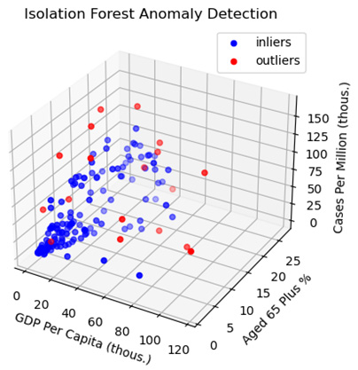
Figure 2.10 – Isolation Forest Anomaly Detection – GDP Per Capita and Cases Per Million
Although we are only able to see three dimensions with this visualization, the plot does illustrate some of what makes an outlier an outlier. We expect cases to increase as the GDP per capita and the age 65 plus percentage increase. We can see that the outliers deviate from the expected pattern, having cases per million noticeably above or below countries with similar GDPs and age 65 plus values.
Summary
In this chapter, we used bivariate and multivariate statistical techniques and visualizations to get a better sense of bivariate relationships among features. We looked at common statistics, such as the Pearson correlation. We also examined bivariate relationships through visualizations, with scatter plots when both features are continuous, and with grouped boxplots when one feature is categorical. The last three sections of this chapter explored multivariate techniques for examining relationships and identifying outliers, including machine learning algorithms such as KNN and Isolation Forest.
Now that we have a good sense of the distribution of our data, we are ready to start engineering our features, including imputing missing values and encoding, transforming, and scaling our variables. This will be our focus for the next two chapters.