
Chapter 10: Logistic Regression
In this and the next few chapters, we will explore models for classification. These involve targets with two or several class values, such as whether a student will pass a class or not or whether a customer will choose chicken, beef, or tofu at a restaurant with only these three choices. There are several machine learning algorithms for these kinds of classification problems. We will take a look at some of the most popular ones in this chapter.
Logistic regression has been used to build models with binary targets for decades. Traditionally, it has been used to generate estimates of the impact of an independent variable or variables on the odds of a dichotomous outcome. Since our focus is on prediction, rather than the effect of each feature, we will also explore regularization techniques, such as lasso regression. These techniques can improve the accuracy of our classification predictions. We will also examine strategies for predicting a multiclass target (when there are more than two possible target values).
In this chapter, we will cover the following topics:
- Key concepts of logistic regression
- Binary classification with logistic regression
- Regularization with logistic regression
- Multinomial logistic regression
Technical requirements
In this chapter, we will stick to the libraries that are available in most scientific distributions of Python: pandas, NumPy, and scikit-learn. All the code in this chapter will run fine with scikit-learn versions 0.24.2 and 1.0.2.
Key concepts of logistic regression
If you are familiar with linear regression, or read Chapter 7, Linear Regression Models, of this book, you have probably anticipated some of the issues we will discuss in this chapter – regularization, linearity among regressors, and normally distributed residuals. If you have built supervised machine learning models in the past or worked through the last few chapters of this book, then you have also likely anticipated that we will spend some time discussing the bias-variance tradeoff and how that influences our choice of model.
I remember being introduced to logistic regression 35 years ago in a college course. It is often presented in undergraduate texts almost as a special case of linear regression; that is, linear regression with a binary dependent variable coupled with some transformation to keep predictions between 0 and 1.
It does share many similarities with linear regression of a numeric target variable. Logistic regression is relatively easy to train and interpret. Optimization techniques for both linear and logistic regression are efficient and can generate low bias predictors.
Also like linear regression, logistic regression predicts a target based on weights assigned to each feature. But to constrain the predicted probability to between 0 and 1, we use the sigmoid function. This function takes any value and maps it to a value between 0 and 1:

As x approaches infinity, ![]() gets closer to 1. As x approaches negative infinity,
gets closer to 1. As x approaches negative infinity, ![]() gets closer to 0.
gets closer to 0.
The following plot illustrates a sigmoid function:
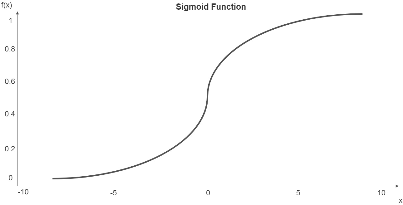
Figure 10.1 – Sigmoid function
We can plug the familiar equation for linear regression, ![]() , into the sigmoid function to predict the probability of class membership:
, into the sigmoid function to predict the probability of class membership:

Here ![]() is the predicted probability of class membership in the binary case. The coefficients (the betas) can be converted into odds ratios for interpretation, as follows:
is the predicted probability of class membership in the binary case. The coefficients (the betas) can be converted into odds ratios for interpretation, as follows:

Here, r is the odds ratio and β is the coefficient. A 1-unit increase in the value of a feature multiplies the odds of class membership by ![]() . Similarly, for a binary feature, a true value has
. Similarly, for a binary feature, a true value has ![]() times the odds of class membership as does a false value for that feature, all else being equal.
times the odds of class membership as does a false value for that feature, all else being equal.
Logistic regression has several advantages as an algorithm for classification problems. Features can be dichotomous, categorical, or numeric, and do not need to be normally distributed. The target variable can have more than two possible values, as we will discuss later, and it can be nominal or ordinal. Another key advantage is that the relationship between features and the target is not assumed to be linear.
The nomenclature here is a tad confusing. Why are we using a regression algorithm for a classification problem? Well, logistic regression predicts the probability of class membership. We apply a decision rule to those probabilities to predict membership. The default threshold is often 0.5 with binary targets. Instances with predicted probabilities greater than or equal to 0.5 get a positive class or 1 or True; those less than 0.5 are assigned 0 or False.
Logistic regression extensions
We will consider two key extensions of logistic regression in this chapter. We will explore multiclass models – that is, those where the target has more than two values. We will also examine the regularization of logistic models to improve (lessen) variance.
A popular choice when constructing multiclass models is multinomial logistic regression (MLR). With MLR, the prediction probability distribution is a multinomial probability distribution. We can replace the equation we used for the binary classifier with a softmax function:

Here, ![]() . This calculates a probability for each class label, j, where k is the number of classes.
. This calculates a probability for each class label, j, where k is the number of classes.
An alternative to multinomial logistic regression when we have more than two classes is one-versus-rest (OVR) logistic regression. This extension to logistic regression turns the multiclass problem into a binary problem, estimating the probability of class membership versus membership in all of the other classes. The key assumption here is that membership in each class is independent. We will use MLR in an example in this chapter. One advantage it has over OVR is that the predicted probabilities are more reliable.
As mentioned previously, logistic regression has some of the same challenges as linear regression, including that the low bias of our predictions comes with high variance. This is more likely to be a problem when several features are highly correlated. Fortunately, we can deal with this with regularization, just as we saw in Chapter 7, Linear Regression Models.
Regularization adds a penalty to the loss function. We still seek to minimize the error, but also constrain the size of our parameters. L1 regularization, also referred to as lasso regression, penalizes the absolute value of the weights (or coefficients):

Here, p is the number of features and λ determines the strength of the regularization. L2 regularization, also referred to as ridge regression, penalizes the squared values of the weights:

Both L1 and L2 regularization push the weights toward 0, though L1 regularization is more likely to lead to sparse models. In scikit-learn, we use the C parameter to adjust the value of λ, where C is just the inverse of λ:

We can get a balance between L1 and L2 with elastic net regression. With elastic net regression, we adjust the L1 ratio. A value of 0.5 uses L1 and L2 equally. We can use hyperparameter tuning to choose the best value for the L1 ratio.
Regularization can result in a model with lower variance, which is a good tradeoff when we are less concerned about our coefficients than we are with our predictions.
Before building a model with regularization, we will construct a fairly straightforward logistic model with a binary target. We will also spend a good amount of time evaluating that model. This will be the first classification model we will build in this book and model evaluation looks very different for those models than it does for regression models.
Binary classification with logistic regression
Logistic regression is often used to model health outcomes when the target is binary, such as whether the person gets a disease or not. We will go through an example of that in this section. We will build a model to predict if an individual will have heart disease based on personal characteristics such as smoking and alcohol drinking habits; health features, including BMI, asthma, diabetes, and skin cancer; and age.
Note
In this chapter, we will work exclusively with data on heart disease that’s available for public download at https://www.kaggle.com/datasets/kamilpytlak/personal-key-indicators-of-heart-disease. This dataset is derived from the United States Center for Disease Control data on more than 400,000 individuals from 2020. Data columns include whether respondents ever had heart disease, body mass index, ever smoked, heavy alcohol drinking, age, diabetes, and kidney disease. We will work with a 30,000 individual sample in this section to speed up the processing, but the full dataset is available in the same folder in this book’s GitHub repository.
We will also do a little more preprocessing in this chapter than we have in previous chapters. We will integrate much of this work with our pipeline. This will make it easier to reuse this code in the future and lessens the likelihood of data leakage. Follow these steps:
- We will start by importing the same libraries we have worked with in the last few chapters. We will also import the LogisticRegression and metrics modules. We will use the metrics module from scikit-learn to evaluate each of our classification models in this part of this book. In addition to matplotlib for visualizations, we will also use seaborn:
import pandas as pd
import numpy as np
from sklearn.model_selection import train_test_split
from sklearn.preprocessing import StandardScaler
from sklearn.preprocessing import OneHotEncoder
from sklearn.pipeline import make_pipeline
from sklearn.impute import SimpleImputer
from sklearn.compose import ColumnTransformer
from sklearn.model_selection import StratifiedKFold
from sklearn.feature_selection import RFECV
from sklearn.linear_model import LogisticRegression
import sklearn.metrics as skmet
import matplotlib.pyplot as plt
import seaborn as sns
- We are also going to need several custom classes to handle the preprocessing. We have already seen the OutlierTrans class. Here, we have added a couple of new classes – MakeOrdinal and ReplaceVals:
import os
import sys
sys.path.append(os.getcwd() + "/helperfunctions")
from preprocfunc import OutlierTrans,
MakeOrdinal, ReplaceVals
The MakeOrdinal class takes a character feature and assigns numeric values based on an alphanumeric sort. For example, a feature that has three possible values – not well, okay, and well – would be transformed into an ordinal feature with values of 0, 1, and 2, respectively.
Recall that scikit-learn pipeline transformers must have fit and transform methods, and must inherit from BaseEstimator. They often also inherit from TransformerMixin, though there are other options.
All the action in the MakeOrdinal class happens in the transform method. We loop over all of the columns that are passed to it by the column transformer. For each column, we find all the unique values and sort them alphanumerically, storing the unique values in a NumPy array that we name cats. Then, we use a lambda function and NumPy’s where method to find the index of cats associated with each feature value:
class MakeOrdinal(BaseEstimator,TransformerMixin):
def fit(self,X,y=None):
return self
def transform(self,X,y=None):
Xnew = X.copy()
for col in Xnew.columns:
cats = np.sort(Xnew[col].unique())
Xnew[col] = Xnew.
apply(lambda x: int(np.where(cats==
x[col])[0]), axis=1)
return Xnew.values
MakeOrdinal will work fine when the alphanumeric order matches a meaningful order, as with the previous example. When that is not true, we can use ReplaceVals to assign appropriate ordinal values. This class replaces values in any feature with alternative values based on a dictionary passed to it.
We could have just used the pandas replace method without putting it in a pipeline, but this way, it is easier to integrate our recoding with other pipeline steps, such as feature scaling:
class ReplaceVals(BaseEstimator,TransformerMixin):
def __init__(self,repdict):
self.repdict = repdict
def fit(self,X,y=None):
return self
def transform(self,X,y=None):
Xnew = X.copy().replace(self.repdict)
return Xnew.values
Do not worry if you do not fully understand how we will use these classes yet. It will be clearer when we add them to our column transformations.
- Next, we will load the heart disease data and take a look at a few rows. Several string features are conceptually binary, such as alcoholdrinkingheavy, which is Yes when the person is a heavy drinker and No otherwise. We will need to encode these features before running a model.
The agecategory feature is character data that represents the age interval. We will need to convert that feature into numeric:
healthinfo = pd.read_csv("data/healthinfo.csv")
healthinfo.set_index("personid", inplace=True)
healthinfo.head(2).T
personid 299391 252786
heartdisease Yes No
bmi 28.48 25.24
smoking Yes Yes
alcoholdrinkingheavy No No
stroke No No
physicalhealthbaddays 7 0
mentalhealthbaddays 0 2
walkingdifficult No No
gender Male Female
agecategory 70-74 65-69
ethnicity White White
diabetic No, borderline diabetes No
physicalactivity Yes Yes
genhealth Good Very good
sleeptimenightly 8 8
asthma No No
kidneydisease No No
skincancer No Yes
- Let’s look at the size of the DataFrame and how many missing values we have. There are 30,000 instances, but there are no missings for any of the 18 data columns. That’s great. We won’t have to worry about that when we construct our pipeline:
healthinfo.shape
(30000, 18)
healthinfo.isnull().sum()
heartdisease 0
bmi 0
smoking 0
alcoholdrinkingheavy 0
stroke 0
physicalhealthbaddays 0
mentalhealthbaddays 0
walkingdifficult 0
gender 0
agecategory 0
ethnicity 0
diabetic 0
physicalactivity 0
genhealth 0
sleeptimenightly 0
asthma 0
kidneydisease 0
skincancer 0
dtype: int64
- Let’s change the heartdisease variable, which will be our target, into a 0 and 1 variable. This will give us one less thing to worry about later. One thing to notice right away is that the target’s values are quite imbalanced. Less than 10% of our observations have heart disease. That, of course, is good news, but it presents some challenges for modeling that we will need to handle:
healthinfo.heartdisease.value_counts()
No 27467
Yes 2533
Name: heartdisease, dtype: int64
healthinfo['heartdisease'] =
np.where(healthinfo.heartdisease=='No',0,1).
astype('int')
healthinfo.heartdisease.value_counts()
0 27467
1 2533
Name: heartdisease, dtype: int64
- We should organize our features by the preprocessing we will be doing with them. We will be scaling the numeric features and doing one-hot encoding with the categorical features. We want to make the agecategory and genhealth features, which are currently strings, into ordinal features.
We need to do a specific cleanup of the diabetic feature. Some individuals indicate no, but that they were borderline. For our purposes, we will consider them a no. Some individuals had diabetes during their pregnancies only. We will consider them a yes. For both genhealth and diabetic, we will set up a dictionary that will indicate how feature values should be replaced. We will use that dictionary in the ReplaceVals transformer of our pipeline:
num_cols = ['bmi','physicalhealthbaddays',
'mentalhealthbaddays','sleeptimenightly']
binary_cols = ['smoking','alcoholdrinkingheavy',
'stroke','walkingdifficult','physicalactivity',
'asthma','kidneydisease','skincancer']
cat_cols = ['gender','ethnicity']
spec_cols1 = ['agecategory']
spec_cols2 = ['genhealth']
spec_cols3 = ['diabetic']
rep_dict = {
'genhealth': {'Poor':0,'Fair':1,'Good':2,
'Very good':3,'Excellent':4},
'diabetic': {'No':0,
'No, borderline diabetes':0,'Yes':1,
'Yes (during pregnancy)':1}
}
- We should take a look at some frequencies for the binary features, as well as other categorical features. A large percentage of the individuals (42%) report that they have been smokers. 14% report that they have difficulty walking:
healthinfo[binary_cols].
apply(pd.value_counts, normalize=True).T
No Yes
smoking 0.58 0.42
alcoholdrinkingheavy 0.93 0.07
stroke 0.96 0.04
walkingdifficult 0.86 0.14
physicalactivity 0.23 0.77
asthma 0.87 0.13
kidneydisease 0.96 0.04
skincancer 0.91 0.09
- Let’s also look at frequencies for the other categorical features. There are nearly equal numbers of men and women. Most people report excellent or very good health:
for col in healthinfo[cat_cols +
['genhealth','diabetic']].columns:
print(col, "----------------------",
healthinfo[col].value_counts(normalize=True).
sort_index(), sep=" ", end=" ")
This produces the following output:
gender
----------------------
Female 0.52
Male 0.48
Name: gender, dtype: float64
ethnicity
----------------------
American Indian/Alaskan Native 0.02
Asian 0.03
Black 0.07
Hispanic 0.09
Other 0.03
White 0.77
Name: ethnicity, dtype: float64
genhealth
----------------------
Excellent 0.21
Fair 0.11
Good 0.29
Poor 0.04
Very good 0.36
Name: genhealth, dtype: float64
diabetic
----------------------
No 0.84
No, borderline diabetes 0.02
Yes 0.13
Yes (during pregnancy) 0.01
Name: diabetic, dtype: float64
- We should also look at some descriptive statistics for the numerical features. The median value for both bad physical health and mental health days is 0; that is, at least half of the observations report no bad physical health days, and at least half report no bad mental health days over the previous month:
healthinfo[num_cols].
agg(['count','min','median','max']).T
count min median max
bmi 30,000 12 27 92
physicalhealthbaddays 30,000 0 0 30
mentalhealthbaddays 30,000 0 0 30
sleeptimenightly 30,000 1 7 24
We will need to do some scaling. We will also need to do some encoding of the categorical features. There are also some extreme values for the numerical features. A sleeptimenightly value of 24 seems unlikely! It is probably a good idea to deal with them.
- Now, we are ready to build our pipeline. Let’s create the training and testing DataFrames:
X_train, X_test, y_train, y_test =
train_test_split(healthinfo[num_cols +
binary_cols + cat_cols + spec_cols1 +
spec_cols2 + spec_cols3],
healthinfo[['heartdisease']], test_size=0.2,
random_state=0)
- Next, we will set up the column transformations. We will create a one-hot encoder instance that we will use for all of the categorical features. For the numeric columns, we will remove extreme values using the OutlierTrans object and then impute the median.
We will convert the agecategory feature into an ordinal one using the MakeOrdinal transformer and code the genhealth and diabetic features using the ReplaceVals transformer.
We will add the column transformation to our pipeline in the next step:
ohe = OneHotEncoder(drop='first', sparse=False)
standtrans = make_pipeline(OutlierTrans(3),
SimpleImputer(strategy="median"),
StandardScaler())
spectrans1 = make_pipeline(MakeOrdinal(),
StandardScaler())
spectrans2 = make_pipeline(ReplaceVals(rep_dict),
StandardScaler())
spectrans3 = make_pipeline(ReplaceVals(rep_dict))
bintrans = make_pipeline(ohe)
cattrans = make_pipeline(ohe)
coltrans = ColumnTransformer(
transformers=[
("stand", standtrans, num_cols),
("spec1", spectrans1, spec_cols1),
("spec2", spectrans2, spec_cols2),
("spec3", spectrans3, spec_cols3),
("bin", bintrans, binary_cols),
("cat", cattrans, cat_cols),
]
)
- Now, we are ready to set up and fit our pipeline. First, we will instantiate logistic regression and stratified k-fold objects, which we will use with recursive feature elimination. Recall that recursive feature elimination needs an estimator. We use stratified k-fold to get approximately the same target value distribution in each fold.
Now, we must create another logistic regression instance for our model. We will set the class_weight parameter to balanced. This should improve the model’s ability to deal with the class imbalance. Then, we will add the column transformation, recursive feature elimination, and logistic regression instance to our pipeline, and then fit it:
lrsel = LogisticRegression(random_state=1,
max_iter=1000)
kf = StratifiedKFold(n_splits=5, shuffle=True)
rfecv = RFECV(estimator=lrsel, cv=kf)
lr = LogisticRegression(random_state=1,
class_weight='balanced', max_iter=1000)
pipe1 = make_pipeline(coltrans, rfecv, lr)
pipe1.fit(X_train, y_train.values.ravel())
- We need to do a little work to recover the column names from the pipeline after the fit. We can use the get_feature_names method of the one-hot encoder for the bin transformer and the cat transformer for this. This gives us the column names for the binary and categorical features after the encoding. The names of the numerical features remain unchanged. We will use the feature names later:
new_binary_cols =
pipe1.named_steps['columntransformer'].
named_transformers_['bin'].
named_steps['onehotencoder'].
get_feature_names(binary_cols)
new_cat_cols =
pipe1.named_steps['columntransformer'].
named_transformers_['cat'].
named_steps['onehotencoder'].
get_feature_names(cat_cols)
new_cols = np.concatenate((np.array(num_cols +
spec_cols1 + spec_cols2 + spec_cols3),
new_binary_cols, new_cat_cols))
new_cols
array(['bmi', 'physicalhealthbaddays',
'mentalhealthbaddays', 'sleeptimenightly',
'agecategory', 'genhealth', 'diabetic',
'smoking_Yes', 'alcoholdrinkingheavy_Yes',
'stroke_Yes', 'walkingdifficult_Yes',
'physicalactivity_Yes', 'asthma_Yes',
'kidneydisease_Yes', 'skincancer_Yes',
'gender_Male', 'ethnicity_Asian',
'ethnicity_Black', 'ethnicity_Hispanic',
'ethnicity_Other', 'ethnicity_White'],
dtype=object)
- Now, let’s look at the results from the recursive feature elimination. We can use the ranking_ attribute of the rfecv object to get the ranking of each feature. Those with a 1 for ranking will be selected for our model.
If we use the get_support method or the support_ attribute of the rfecv object instead of the ranking_ attribute, we get just those features that will be used in our model – that is, those with a ranking of 1. We will do that in the next step:
rankinglabs =
np.column_stack((pipe1.named_steps['rfecv'].ranking_,
new_cols))
pd.DataFrame(rankinglabs,
columns=['rank','feature']).
sort_values(['rank','feature']).
set_index("rank")
feature
rank
1 agecategory
1 alcoholdrinkingheavy_Yes
1 asthma_Yes
1 diabetic
1 ethnicity_Asian
1 ethnicity_Other
1 ethnicity_White
1 gender_Male
1 genhealth
1 kidneydisease_Yes
1 smoking_Yes
1 stroke_Yes
1 walkingdifficult_Yes
2 ethnicity_Hispanic
3 skincancer_Yes
4 bmi
5 physicalhealthbaddays
6 sleeptimenightly
7 mentalhealthbaddays
8 physicalactivity_Yes
9 ethnicity_Black
- We can get the odds ratios from the coefficients from the logistic regression. Recall that the odds ratio is the exponentiated coefficient. There are 13 coefficients, which makes sense because we learned in the previous step that 13 features got a ranking of 1.
We will use the get_support method of the rfecv step to get the names of the selected features and create a NumPy array with those names and the odds ratios, oddswithlabs. We then create a pandas DataFrame and sort by the odds ratio in descending order.
Not surprisingly, those who had a stroke and older individuals are substantially more likely to have heart disease. If the individual had a stroke, they had three times the odds of having heart disease, controlling for everything else. The odds of having heart disease increase by 2.88 times for each increase in age category. On the other hand, the odds of having heart disease decline by about half (57%) for every increase in general health; from, say, fair to good. Surprisingly, heavy alcohol drinking is associated with lower odds of heart disease, controlling for everything else:
oddsratios = np.exp(pipe1.
named_steps['logisticregression'].coef_)
oddsratios.shape
(1, 13)
selcols = new_cols[pipe1.
named_steps['rfecv'].get_support()]
oddswithlabs = np.column_stack((oddsratios.
ravel(), selcols))
pd.DataFrame(oddswithlabs,
columns=['odds','feature']).
sort_values(['odds'], ascending=False).
set_index('odds')
feature
odds
3.01 stroke_Yes
2.88 agecategory
2.12 gender_Male
1.97 kidneydisease_Yes
1.75 diabetic
1.55 smoking_Yes
1.52 asthma_Yes
1.30 walkingdifficult_Yes
1.27 ethnicity_Other
1.22 ethnicity_White
0.72 ethnicity_Asian
0.61 alcoholdrinkingheavy_Yes
0.57 genhealth
Now that we have fit our logistic regression model, we are ready to evaluate it. In the next section, we will spend some time looking into various performance measures, including accuracy and sensitivity. We will use many of the concepts that we introduced in Chapter 6, Preparing for Model Evaluation.
Evaluating a logistic regression model
The most intuitive measure of a classification model’s performance is its accuracy – that is, how often our predictions are correct. In some cases, however, we might be at least as concerned about sensitivity – the percent of positive cases that we predict correctly – as accuracy; we may even be willing to lose a little accuracy to improve sensitivity. Predictive models of diseases often fall into that category. But whenever there is a class imbalance, measures such as accuracy and sensitivity can give us very different estimates of the performance of our model.
In addition to being concerned about accuracy or sensitivity, we might be worried about our model’s specificity or precision. We may want a model that can identify negative cases with high reliability, even if that means it does not do as good a job of identifying positives. Specificity is a measure of the percentage of all negatives identified by the model.
Precision, which is the percentage of predicted positives that are positives, is another important measure. For some applications, it is important to limit false positives, even if we have to tolerate lower sensitivity. An apple grower, using image recognition to identify bad apples, may prefer a high-precision model to a more sensitive one, not wanting to discard apples unnecessarily.
This can be made more clear by looking at a confusion matrix:
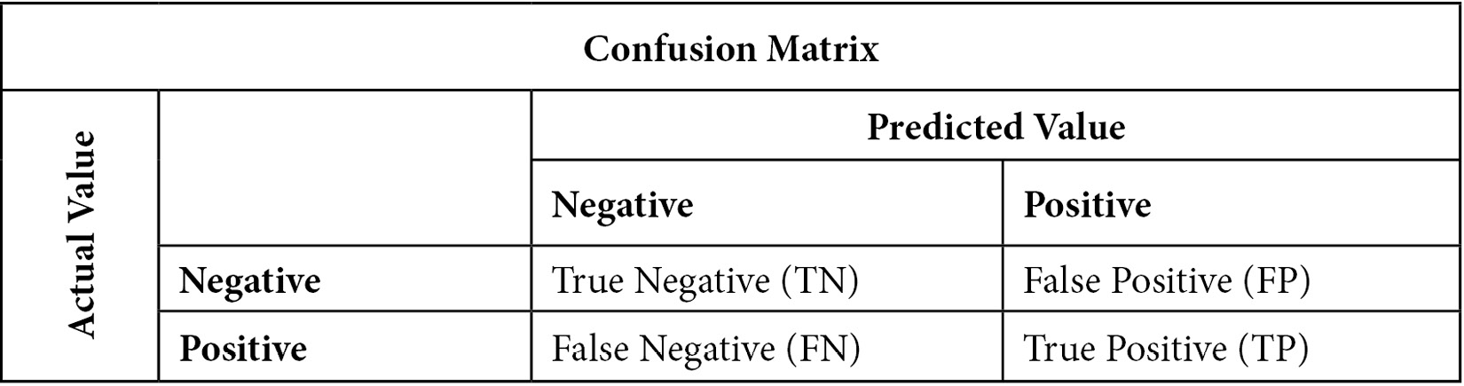
Figure 10.2 – Confusion matrix of actual by predicted values for a binary target
The confusion matrix helps us conceptualize accuracy, sensitivity, specificity, and precision. Accuracy is the percentage of observations for which our prediction was correct. This can be stated more precisely as follows:

Sensitivity is the number of times we predicted positives correctly divided by the number of positives. It might be helpful to glance at the confusion matrix again and confirm that actual positive values can either be predicted positives (TP) or predicted negatives (FN). Sensitivity is also referred to as recall or the true positive rate:

Specificity is the number of times we correctly predicted a negative value (TN) divided by the number of actual negative values (TN + FP). Specificity is also known as the true negative rate:

Precision is the number of times we correctly predicted a positive value (TP) divided by the number of positive values predicted:

We went over these concepts in more detail in Chapter 6, Preparing for Model Evaluation. In this section, we will examine the accuracy, sensitivity, specificity, and precision of our logistic regression model of heart disease:
- We can use the predict method of the pipeline we fitted in the previous section to generate predictions from our logistic regression. Then, we can generate a confusion matrix:
pred = pipe1.predict(X_test)
cm = skmet.confusion_matrix(y_test, pred)
cmplot = skmet.ConfusionMatrixDisplay(confusion_matrix=cm, display_labels=['Negative', 'Positive'])
cmplot.plot()
cmplot.ax_.set(title='Heart Disease Prediction Confusion Matrix',
xlabel='Predicted Value', ylabel='Actual Value')
This produces the following plot:

Figure 10.3 – A confusion matrix for heart disease prediction
The first thing to notice here is that most of the action is in the top-left quadrant, where we correctly predict actual negative values in the testing data. That is going to help our accuracy a fair bit. Nonetheless, we have a fair number of false positives. We predict heart disease 1,430 times (out of 5,506 negative instances) when there is no heart disease. We do seem to do an okay job of identifying positive heart disease instances, correctly classifying 392 instances (out of 494) that were positive.
- Let’s calculate the accuracy, sensitivity, specificity, and precision. The overall accuracy is not great, at 74%. Sensitivity is pretty decent though, at 79%. (Of course, how decent the sensitivity is depends on the domain and judgment. For something such as heart disease, we likely want it to be higher.) This can be seen in the following code:
tn, fp, fn, tp = skmet.confusion_matrix(y_test.values.ravel(), pred).ravel()
tn, fp, fn, tp
(4076, 1430, 102, 392)
accuracy = (tp + tn) / pred.shape[0]
accuracy
0.7446666666666667
sensitivity = tp / (tp + fn)
sensitivity
0.7935222672064778
specificity = tn / (tn+fp)
specificity
0.7402833272793317
precision = tp / (tp + fp)
precision
0.21514818880351264
- We can do these calculations in a more straightforward way using the metrics module (I chose a more roundabout approach in the previous step to illustrate how the calculations are done):
print("accuracy: %.2f, sensitivity: %.2f, specificity: %.2f, precision: %.2f" %
(skmet.accuracy_score(y_test.values.ravel(), pred),
skmet.recall_score(y_test.values.ravel(), pred),
skmet.recall_score(y_test.values.ravel(), pred,
pos_label=0),
skmet.precision_score(y_test.values.ravel(), pred)))
accuracy: 0.74, sensitivity: 0.79, specificity: 0.74, precision: 0.22
The biggest problem with our model is the very low level of precision – that is, 22%. This is due to the large number of false positives. The majority of the time that our model predicts positive, it is wrong.
In addition to the four measures that we have already calculated, it can also be helpful to get the false positive rate. The false positive rate is the propensity of our model to predict positive when the actual value is negative:

- Let’s calculate the false positive rate:
falsepositiverate = fp / (tn + fp)
falsepositiverate
0.25971667272066834
So, 26% of the time that a person does not have heart disease, we predicted that they do. While we certainly want to limit the number of false positives, this often means sacrificing some sensitivity. We will demonstrate why this is true later in this section.
- We should take a closer look at the prediction probabilities generated by our model. Here, the threshold for a positive class prediction is 0.5, which is often the default with logistic regression. (Recall that logistic regression predicts a probability of class membership. We need an accompanying decision rule, such as the 0.5 threshold, to predict the class.) This can be seen in the following code:
pred_probs = pipe1.predict_proba(X_test)[:, 1]
probdf =
pd.DataFrame(zip(pred_probs, pred,
y_test.values.ravel()),
columns=(['prob','pred','actual']))
probdf.groupby(['pred'])['prob'].
agg(['min','max','count'])
min max count
pred
0 0.01 0.50 4178
1 0.50 0.99 1822
- We can use a kernel density estimate (KDE) plot to visualize these probabilities. We can also see how a different decision rule may impact our predictions. For example, we could move the threshold from 0.5 to 0.25. At a glance, that has some advantages. The area between the two possible thresholds has somewhat more heart disease cases than no heart disease cases. We would be getting the brown area between the dashed lines right, predicting heart disease correctly where we would not have with the 0.5 threshold. That is a larger area than the green area between the lines, where we turn some of the true negative predictions at the 0.5 threshold into false positives at the 0.25 threshold:
sns.kdeplot(probdf.loc[probdf.actual==1].prob,
shade=True, color='red',label="Heart Disease")
sns.kdeplot(probdf.loc[probdf.actual==0].prob,
shade=True,color='green',label="No Heart Disease")
plt.axvline(0.25, color='black', linestyle='dashed',
linewidth=1)
plt.axvline(0.5, color='black', linestyle='dashed',
linewidth=1)
plt.title("Predicted Probability Distribution")
plt.legend(loc="upper left")
This generates the following plot:

Figure 10.4 – Heart disease predicted probability distribution
Let’s consider the tradeoff between precision and sensitivity a little more carefully than we have so far. Remember that precision is the rate at which we are right when we predict a positive class value. Sensitivity, also referred to as recall or the true positive rate, is the rate at which we identify an actual positive as positive.
- We can plot precision and sensitivity curves as follows:
prec, sens, ths = skmet.precision_recall_curve(y_test, pred_probs)
sens = sens[1:-20]
prec = prec[1:-20]
ths = ths[:-20]
fig, ax = plt.subplots()
ax.plot(ths, prec, label='Precision')
ax.plot(ths, sens, label='Sensitivity')
ax.set_title('Precision and Sensitivity by Threshold')
ax.set_xlabel('Threshold')
ax.set_ylabel('Precision and Sensitivity')
ax.legend()
This generates the following plot:

Figure 10.5 – Precision and sensitivity at threshold values
As the threshold increases beyond 0.2, there is a sharper decrease in sensitivity than there is an increase in precision.
- It is often also helpful to look at the false positive rate with the sensitivity rate. The false positive rate is the propensity of our model to predict positive when the actual value is negative. One way to see that relationship is with a ROC curve:
fpr, tpr, ths = skmet.roc_curve(y_test, pred_probs)
ths = ths[1:]
fpr = fpr[1:]
tpr = tpr[1:]
fig, ax = plt.subplots()
ax.plot(fpr, tpr, linewidth=4, color="black")
ax.set_title('ROC curve')
ax.set_xlabel('False Positive Rate')
ax.set_ylabel('Sensitivity')
This produces the following plot:

Figure 10.6 – ROC curve
Here, we can see that increasing the false positive rate buys us less increase in sensitivity the higher the false positive rate is. Beyond a false positive rate of 0.5, there is not much payoff at all.
- It may also be helpful to just plot the false positive rate and sensitivity by threshold:
fig, ax = plt.subplots()
ax.plot(ths, fpr, label="False Positive Rate")
ax.plot(ths, tpr, label="Sensitivity")
ax.set_title('False Positive Rate and Sensitivity by Threshold')
ax.set_xlabel('Threshold')
ax.set_ylabel('False Positive Rate and Sensitivity')
ax.legend()
This produces the following plot:
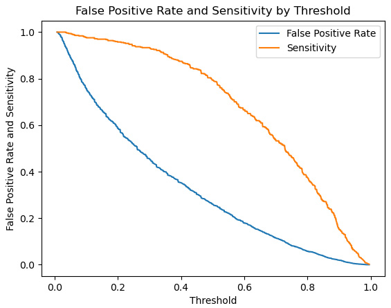
Figure 10.7 – Sensitivity and false positive rate
Here, we can see that as we lower the threshold below 0.25, the false positive rate increases more rapidly than sensitivity.
These last two visualizations hint at the possibility of finding an optimal threshold value – that is, one with the best tradeoff between sensitivity and the false positive rate; at least mathematically, ignoring domain knowledge.
- We will calculate the Youden J statistic to find this threshold value. We get this by passing a vector, which is the difference between the true positive and false positive rates at each threshold, to NumPy’s argmax function. We want the value of the threshold at that index. The optimal threshold according to this calculation is 0.46, which isn’t very different from the default:
jthresh = ths[np.argmax(tpr – fpr)]
jthresh
0.45946882675453804
- We can redo the confusion matrix based on this alternative threshold:
pred2 = np.where(pred_probs>=jthresh,1,0)
cm = skmet.confusion_matrix(y_test, pred2)
cmplot = skmet.ConfusionMatrixDisplay(
confusion_matrix=cm,
display_labels=['Negative', 'Positive'])
cmplot.plot()
cmplot.ax_.set(
title='Heart Disease Prediction Confusion Matrix',
xlabel='Predicted Value', ylabel='Actual Value')
This produces the following plot:

Figure 10.8 – Confusion matrix of heart disease prediction
- This gives us a small improvement in sensitivity:
skmet.recall_score(y_test.values.ravel(), pred)
0.7935222672064778
skmet.recall_score(y_test.values.ravel(), pred2)
0.8380566801619433
The point here is not that we should change thresholds willy-nilly. This is often a bad idea. But we should keep two points in mind. First, when we have a highly imbalanced class, a 0.5 threshold may not make sense. Second, this is an important place to lean on domain knowledge. For some classification problems, a false positive is substantially less important than a false negative.
In this section, we focused on sensitivity, precision, and false positive rate as measures of model performance. That is partly because of space limitations, but also because of the issues with this particular target – imbalance classes and the likely preference for sensitivity. We will be emphasizing other measures, such as accuracy and specificity, in other models that we will be building in the next few chapters. In the rest of this chapter, we will look at a couple of extensions of logistic regression, regularization and multinomial logistic regression.
Regularization with logistic regression
If you have already worked your way through Chapter 7, Linear Regression Models, and read the first section of this chapter, you already have a good idea of how regularization works. We add a penalty to the estimator that minimizes our parameter estimates. The size of that penalty is typically tuned based on a measure of model performance. We will work through that in this section. Follow these steps:
- We will load the same modules that we worked with in the previous section, plus the modules we will need for the necessary hyperparameter tuning. We will use RandomizedSearchCV and uniform to find the best value for our penalty strength:
import pandas as pd
import numpy as np
from sklearn.model_selection import train_test_split
from sklearn.preprocessing import StandardScaler
from sklearn.preprocessing import OneHotEncoder
from sklearn.pipeline import make_pipeline
from sklearn.impute import SimpleImputer
from sklearn.compose import ColumnTransformer
from sklearn.model_selection import RepeatedStratifiedKFold
from sklearn.linear_model import LogisticRegression
from sklearn.model_selection import RandomizedSearchCV
from scipy.stats import uniform
import os
import sys
sys.path.append(os.getcwd() + "/helperfunctions")
from preprocfunc import OutlierTrans,
MakeOrdinal, ReplaceVals
- Next, we will load the heart disease data and do a little processing:
healthinfo = pd.read_csv("data/healthinfosample.csv")
healthinfo.set_index("personid", inplace=True)
healthinfo['heartdisease'] =
np.where(healthinfo.heartdisease=='No',0,1).
astype('int')
- Next, we will organize our features to facilitate the column transformation we will do in a couple of steps:
num_cols = ['bmi','physicalhealthbaddays',
'mentalhealthbaddays','sleeptimenightly']
binary_cols = ['smoking','alcoholdrinkingheavy',
'stroke','walkingdifficult','physicalactivity',
'asthma','kidneydisease','skincancer']
cat_cols = ['gender','ethnicity']
spec_cols1 = ['agecategory']
spec_cols2 = ['genhealth']
spec_cols3 = ['diabetic']
rep_dict = {
'genhealth': {'Poor':0,'Fair':1,'Good':2,
'Very good':3,'Excellent':4},
'diabetic': {'No':0,
'No, borderline diabetes':0,'Yes':1,
'Yes (during pregnancy)':1}
}
- Now, we must create testing and training DataFrames:
X_train, X_test, y_train, y_test =
train_test_split(healthinfo[num_cols +
binary_cols + cat_cols + spec_cols1 +
spec_cols2 + spec_cols3],
healthinfo[['heartdisease']], test_size=0.2,
random_state=0)
- Then, we must set up the column transformations:
ohe = OneHotEncoder(drop='first', sparse=False)
standtrans = make_pipeline(OutlierTrans(3),
SimpleImputer(strategy="median"),
StandardScaler())
spectrans1 = make_pipeline(MakeOrdinal(),
StandardScaler())
spectrans2 = make_pipeline(ReplaceVals(rep_dict),
StandardScaler())
spectrans3 = make_pipeline(ReplaceVals(rep_dict))
bintrans = make_pipeline(ohe)
cattrans = make_pipeline(ohe)
coltrans = ColumnTransformer(
transformers=[
("stand", standtrans, num_cols),
("spec1", spectrans1, spec_cols1),
("spec2", spectrans2, spec_cols2),
("spec3", spectrans3, spec_cols3),
("bin", bintrans, binary_cols),
("cat", cattrans, cat_cols),
]
)
- Now, we are ready to run our model. We will instantiate logistic regression and repeated stratified k-fold objects. Then, we will create a pipeline with our column transformation from the previous step and the logistic regression.
After that, we will create a list of dictionaries for our hyperparameters, rather than just one dictionary, as we have done previously in this book. This is because not all hyperparameters work together. For example, we cannot use an L1 penalty with a newton-cg solver. The logisticregression__ (note the double underscore) prefix to the dictionary key names indicates that we want the values to be passed to the logistic regression step of our pipeline.
We will set the n_iter parameter to 20 for our randomized grid search to get it to sample hyperparameters 20 times. Each of those times, the grid search will select from the hyperparameters listed in one of the dictionaries. We will indicate that we want the grid search scoring to be based on the area under the ROC curve:
lr = LogisticRegression(random_state=1, class_weight='balanced', max_iter=1000)
kf = RepeatedStratifiedKFold(n_splits=7, n_repeats=3, random_state=0)
pipe1 = make_pipeline(coltrans, lr)
reg_params = [
{
'logisticregression__solver': ['liblinear'],
'logisticregression__penalty': ['l1','l2'],
'logisticregression__C': uniform(loc=0, scale=10)
},
{
'logisticregression__solver': ['newton-cg'],
'logisticregression__penalty': ['l2'],
'logisticregression__C': uniform(loc=0, scale=10)
},
{
'logisticregression__solver': ['saga'],
'logisticregression__penalty': ['elasticnet'],
'logisticregression__l1_ratio': uniform(loc=0, scale=1),
'logisticregression__C': uniform(loc=0, scale=10)
}
]
rs = RandomizedSearchCV(pipe1, reg_params, cv=kf,
n_iter=20, scoring='roc_auc')
rs.fit(X_train, y_train.values.ravel())
- After fitting the search, the best_params attribute gives us the parameters associated with the highest score. Elastic net regression, with an L1 ratio closer to L1 than to L2, performs the best:
rs.best_params_
{'logisticregression__C': 0.6918282397356423,
'logisticregression__l1_ratio': 0.758705704020254,
'logisticregression__penalty': 'elasticnet',
'logisticregression__solver': 'saga'}
rs.best_score_
0.8410275986723489
- Let’s look at some of the other top scores from the grid search. The best three models have pretty much the same score. One uses elastic net regression, another L1, and another L2.
The cv_results_ dictionary of the grid search provides us with lots of information about the 20 models that were tried. The params list in that dictionary has a somewhat complicated structure because some keys are not present for some iterations, such as L1_ratio. We can use json_normalize to flatten the structure:
results =
pd.DataFrame(rs.cv_results_['mean_test_score'],
columns=['meanscore']).
join(pd.json_normalize(rs.cv_results_['params'])).
sort_values(['meanscore'], ascending=False)
results.head(3).T
15 4 12
meanscore 0.841 0.841 0.841
logisticregression__C 0.692 1.235 0.914
logisticregression__l1_ratio 0.759 NaN NaN
logisticregression__penalty elasticnet l1 l2
logisticregression__solver saga liblinear liblinear
- Let’s take a look at the confusion matrix:
pred = rs.predict(X_test)
cm = skmet.confusion_matrix(y_test, pred)
cmplot =
skmet.ConfusionMatrixDisplay(confusion_matrix=cm,
display_labels=['Negative', 'Positive'])
cmplot.plot()
cmplot.ax_.
set(title='Heart Disease Prediction Confusion Matrix',
xlabel='Predicted Value', ylabel='Actual Value')
This generates the following plot:
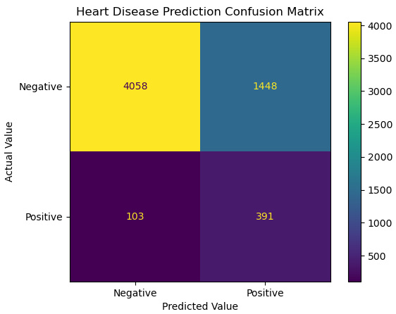
Figure 10.9 – Confusion matrix of heart disease prediction
- Let’s also look at some metrics. Our scores are largely unchanged from our model without regularization:
print("accuracy: %.2f, sensitivity: %.2f, specificity: %.2f, precision: %.2f" %
(skmet.accuracy_score(y_test.values.ravel(), pred),
skmet.recall_score(y_test.values.ravel(), pred),
skmet.recall_score(y_test.values.ravel(), pred,
pos_label=0),
skmet.precision_score(y_test.values.ravel(), pred)))
accuracy: 0.74, sensitivity: 0.79, specificity: 0.74, precision: 0.21
Even though regularization provided no obvious improvement in the performance of our model, there are many times when it does. It is also not as necessary to worry about feature selection when using L1 regularization, as the weights for less important features will be 0.
We still haven’t dealt with how to handle models where the target has more than two possible values, though almost all the discussion in the last two sections applies to multiclass models as well. In the next section, we will learn how to use multinomial logistic regression to model multiclass targets.
Multinomial logistic regression
Logistic regression would not be as useful if it only worked for binary classification problems. Fortunately, we can use multinomial logistic regression when our target has more than two values.
In this section, we will work with data on machine failures as a function of air and process temperature, torque, and rotational speed.
Note
This dataset on machine failure is available for public use at https://www.kaggle.com/datasets/shivamb/machine-predictive-maintenance-classification. There are 10,000 observations, 12 features, and two possible targets. One is binary – that is, the machine failed or didn’t. The other has types of failure. The instances in this dataset are synthetic, generated by a process designed to mimic machine failure rates and causes.
Let’s learn how to use multinomial logistic regression to model machine failure:
- First, we will import the now-familiar libraries. We will also import cross_validate, which we first used in Chapter 6, Preparing for Model Evaluation, to help us evaluate our model:
import pandas as pd
import numpy as np
from sklearn.model_selection import train_test_split
from sklearn.preprocessing import StandardScaler
from sklearn.preprocessing import OneHotEncoder
from sklearn.pipeline import make_pipeline
from sklearn.impute import SimpleImputer
from sklearn.compose import ColumnTransformer
from sklearn.model_selection import RepeatedStratifiedKFold
from sklearn.linear_model import LogisticRegression
from sklearn.model_selection import cross_validate
import os
import sys
sys.path.append(os.getcwd() + "/helperfunctions")
from preprocfunc import OutlierTrans
- We will load the machine failure data and take a look at its structure. We do not have any missing data. That’s great news:
machinefailuretype = pd.read_csv("data/machinefailuretype.csv")
machinefailuretype.info()
<class 'pandas.core.frame.DataFrame'>
RangeIndex: 10000 entries, 0 to 9999
Data columns (total 10 columns):
# Column Non-Null Count Dtype
--- ------ -------------- ----
0 udi 10000 non-null int64
1 product 10000 non-null object
2 machinetype 10000 non-null object
3 airtemp 10000 non-null float64
4 processtemperature 10000 non-null float64
5 rotationalspeed 10000 non-null int64
6 torque 10000 non-null float64
7 toolwear 10000 non-null int64
8 fail 10000 non-null int64
9 failtype 10000 non-null object
dtypes: float64(3), int64(4), object(3)
memory usage: 781.4+ KB
- Let’s look at a few rows. machinetype has values of L, M, and H. These values are proxies for machines of low, medium, and high quality, respectively:
machinefailuretype.head()
udi product machinetype airtemp processtemperature
0 1 M14860 M 298 309
1 2 L47181 L 298 309
2 3 L47182 L 298 308
3 4 L47183 L 298 309
4 5 L47184 L 298 309
Rotationalspeed torque toolwear fail failtype
0 1551 43 0 0 No Failure
1 1408 46 3 0 No Failure
2 1498 49 5 0 No Failure
3 1433 40 7 0 No Failure
4 1408 40 9 0 No Failure
- We should also generate some frequencies:
machinefailuretype.failtype.value_counts(dropna=False).sort_index()
Heat Dissipation Failure 112
No Failure 9652
Overstrain Failure 78
Power Failure 95
Random Failures 18
Tool Wear Failure 45
Name: failtype, dtype: int64
machinefailuretype.machinetype.
value_counts(dropna=False).sort_index()
H 1003
L 6000
M 2997
Name: machinetype, dtype: int64
- Let’s collapse the failtype values and create numeric code for them. We will combine random failures and tool wear failures since the counts are so low for random failures:
def setcode(typetext):
if (typetext=="No Failure"):
typecode = 1
elif (typetext=="Heat Dissipation Failure"):
typecode = 2
elif (typetext=="Power Failure"):
typecode = 3
elif (typetext=="Overstrain Failure"):
typecode = 4
else:
typecode = 5
return typecode
machinefailuretype["failtypecode"] =
machinefailuretype.apply(lambda x: setcode(x.failtype), axis=1)
- We should confirm that failtypecode does what we intended:
machinefailuretype.groupby(['failtypecode','failtype']).size().
reset_index()
failtypecode failtype 0
0 1 No Failure 9652
1 2 Heat Dissipation Failure 112
2 3 Power Failure 95
3 4 Overstrain Failure 78
4 5 Random Failures 18
5 5 Tool Wear Failure 45
- Let’s also get some descriptive statistics:
num_cols = ['airtemp','processtemperature','rotationalspeed',
'torque','toolwear']
cat_cols = ['machinetype']
machinefailuretype[num_cols].agg(['min','median','max']).T
min median max
airtemp 295 300 304
processtemperature 306 310 314
rotationalspeed 1,168 1,503 2,886
torque 4 40 77
toolwear 0 108 253
- Now, let’s create the testing and training DataFrames. We will also set up the column transformations:
X_train, X_test, y_train, y_test =
train_test_split(machinefailuretype[num_cols +
cat_cols], machinefailuretype[['failtypecode']],
test_size=0.2, random_state=0)
ohe = OneHotEncoder(drop='first', sparse=False)
standtrans = make_pipeline(OutlierTrans(3),
SimpleImputer(strategy="median"),
StandardScaler())
cattrans = make_pipeline(ohe)
coltrans = ColumnTransformer(
transformers=[
("stand", standtrans, num_cols),
("cat", cattrans, cat_cols),
]
)
- Now, let’s set up a pipeline with our column transformations and our multinomial logistic regression model We just need to set the multi_class attribute to multinomial when we instantiate the logistic regression:
lr = LogisticRegression(random_state=0,
multi_class='multinomial', solver='lbfgs',
max_iter=1000)
kf = RepeatedStratifiedKFold(n_splits=10,
n_repeats=5, random_state=0)
pipe1 = make_pipeline(coltrans, lr)
- Now, we can generate a confusion matrix:
cm = skmet.confusion_matrix(y_test,
pipe1.fit(X_train, y_train.values.ravel()).
predict(X_test))
cmplot =
skmet.ConfusionMatrixDisplay(confusion_matrix=cm,
display_labels=['None', 'Heat','Power','Overstrain','Other'])
cmplot.plot()
cmplot.ax_.
set(title='Machine Failure Type Confusion Matrix',
xlabel='Predicted Value', ylabel='Actual Value')
This produces the following plot:
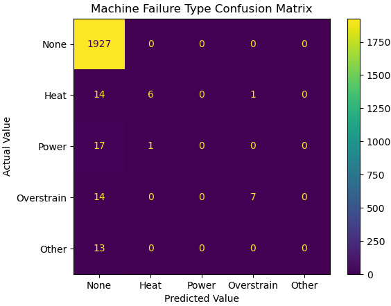
Figure 10.10 – Confusion matrix of predicted machine failure types
The confusion matrix shows that our model does not do a good job of predicting the failure type when there is a failure, particularly with power failures or other failures.
- We can use cross_validate to evaluate this model. We mainly get excellent scores for accuracy, precision, and sensitivity (recall). However, this is misleading. The weighted scores when the classes are so imbalanced (almost all of the instances have no failure) are very heavily influenced by the class that contains almost all of the values. Our model gets no failure correct reliably.
If we look at the f1_macro score (recall from Chapter 6, Preparing for Model Evaluation, that f1 is the harmonic mean of precision and sensitivity), we will see that our model does not do very well for classes other than the no failure class. (The macro score is just a simple average.)
We could have just used a classification report here, as we did in Chapter 6, Preparing for Model Evaluation, but I sometimes find it helpful to generate the stats I need:
scores = cross_validate(
pipe1, X_train, y_train.values.ravel(),
scoring=['accuracy', 'precision_weighted',
'recall_weighted', 'f1_macro',
'f1_weighted'],
cv=kf, n_jobs=-1)
accuracy, precision, sensitivity, f1_macro, f1_weighted =
np.mean(scores['test_accuracy']),
np.mean(scores['test_precision_weighted']),
np.mean(scores['test_recall_weighted']),
np.mean(scores['test_f1_macro']),
np.mean(scores['test_f1_weighted'])
accuracy, precision, sensitivity, f1_macro, f1_weighted
(0.9716499999999999,
0.9541025493784612,
0.9716499999999999,
0.3820938909478524,
0.9611411229222823)
In this section, we explored how to construct a multinomial logistic regression model. This approach works regardless of whether the target is nominal or ordinal. In this case, it was nominal. We also saw how we can extend the model evaluation approaches we used for logistic regression with a binary target. We reviewed how to interpret the confusion matrix and scoring metrics when we have more than two classes.
Summary
Logistic regression has been a go-to tool for me for many, many years when I have needed to predict a categorical target. It is an efficient algorithm with low bias. Some of its disadvantages, such as high variance and difficulty handling highly correlated predictors, can be addressed with regularization and feature selection. We went over examples of doing that in this chapter. We also examined how to handle imbalanced classes in terms of what such targets mean for modeling and interpretation of results.
In the next chapter, we will look at a very popular alternative to logistic regression for classification – decision trees. We will see that decision trees have many advantages that make them a particularly good option if we need to model complexity, without having to worry as much about how our features are specified as we do with logistic regression.