Chapter 6: Preparing for Model Evaluation

It is a good idea to think through how you will evaluate your model’s performance before you begin to run it. A common technique is to separate data into training and testing datasets. We do this relatively early in the process to avoid what is known as data leakage; that is, conducting analyses based on data that is intended to be set aside for model evaluation. In this chapter, we will look at approaches for creating training datasets, including how to ensure that training data is representative. We will look into cross-validation strategies such as K-fold, which address some of the limitations of using static training/testing splits. We will also begin to look more closely at assessing the performance of models.

You might be wondering why we are discussing model evaluation before going over any algorithms in detail. This is because there is a practical consideration. We tend to use the same metrics and evaluation techniques across algorithms with similar purposes. We examine accuracy and sensitivity when evaluating classification models, and mean absolute error and R-squared when examining regression models. We do cross-validation with all supervised learning models. So, we will repeat the strategies introduced here several times in the following chapters. You may even find yourself coming back to these pages when the concepts are re-introduced later.

Beyond those practical considerations, our modeling work improves when we do not see data extraction, data cleaning, exploratory analysis, feature engineering and Preprocessing, model specification, and model evaluation as discrete, sequential tasks. If you have been building machine learning models for just 6 months or over 30 years, you probably appreciate that such rigid sequencing is inconsistent with our workflow as data scientists. We are always preparing for model validation, and always cleaning data. This is a good thing. We do better work when we integrate these tasks; when we continue to interrogate our data cleaning as we select features, and when we look back at bivariate correlations or scatter plots after calculating precision or root mean squared error.

We will also spend a fair bit of time constructing visualizations of these concepts. It is a good idea to get in the habit of looking at confusion matrices and cumulative accuracy profiles when working on classification problems, and plots of residuals when working with a continuous target. This, too, will serve us well in subsequent chapters.

Specifically, in this chapter, we will cover the following topics:

• Measuring accuracy, sensitivity, specificity, and precision for binary classification
• Examining CAP, ROC, and precision-sensitivity curves for binary classification
• Evaluating multiclass models
• Evaluating regression models
• Using K-fold cross-validation
• Preprocessing data with pipelines

Technical requirements

In this chapter, we will work with the feature_engine and matplotlib libraries, in addition to the scikit-learn library. You can use pip to install these packages. The code files for this chapter can be found in this book’s GitHub repository at https://github.com/PacktPublishing/Data-Cleaning-and-Exploration-with-Machine-Learning.

Measuring accuracy, sensitivity, specificity, and precision for binary classification

When assessing a classification model, we typically want to know how often we are right. In the case of a binary target – one where the target has two possible categorical values – we calculate accuracy as the ratio of times we predict the correct classification against the total number of observations.

But, depending on the classification problem, accuracy may not be the most important performance measure. Perhaps we are willing to accept more false positives for a model that can identify more true positives, even if that means lower accuracy. This might be true for a model that would predict the likelihood of having breast cancer, a security breach, or structural damage in a bridge. In these cases, we may emphasize sensitivity (the propensity to identify positive cases) over accuracy.

On the other hand, we may want a model that could identify negative cases with high reliability, even if that meant it did not do as good a job of identifying positives. Specificity is a measure of the percentage of all negatives identified by the model.

Precision, the percentage of predicted positives that are actually positives, is another important measure. For some applications, it is important to limit false positives, even if we have to tolerate lower sensitivity. An apple grower, using image recognition to identify bad apples, may prefer a high-precision model to a more sensitive one, not wanting to discard apples unnecessarily.

This can be made clearer by looking at a confusion matrix:

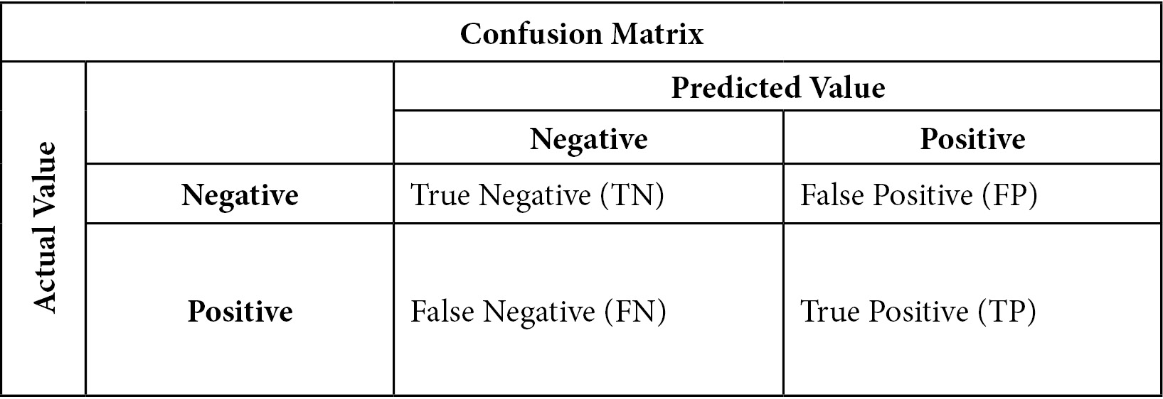
Figure 6.1 – Confusion matrix

The confusion matrix helps us conceptualize accuracy, sensitivity, specificity, and precision. Accuracy is the percentage of observations for which our prediction was correct. This can be stated more precisely as follows:

Sensitivity is the number of times we predicted positives correctly divided by the number of positives. It might be helpful to glance again at the confusion matrix and confirm that actual positive values can either be predicted positives (TP) or predicted negatives (FN). Sensitivity is also referred to as recall or the true positive rate:

Specificity is the number of times we correctly predicted a negative value (TN) divided by the number of actual negative values (TN + FP). Specificity is also known as the true negative rate:

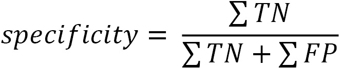
Precision is the number of times we correctly predicted a positive value (TP) divided by the number of positive values predicted:

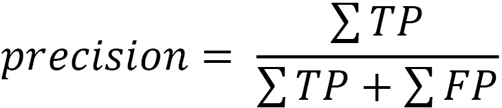
When there is class imbalance, measures such as accuracy and sensitivity can give us very different estimates of the performance of our model. An extreme example will illustrate this. Chimpanzees sometimes termite fish, putting a stick in a termite mound with the hopes of catching a few termites. This is only occasionally successful. I am no primatologist, but we can perhaps model a successful fishing attempt as a function of the size of the stick used, the time of year, and the age of the chimpanzee. In our testing data, fishing attempts are only successful 2% of the time. (This data has been made up for this demonstration.)

Let’s also say that we build a classification model of successful termite fishing that has a sensitivity of 50%. So, if there are 100 fishing attempts in our testing data, we would predict only one of the two successful attempts correctly. There is also one false positive, where our model predicted successful fishing when the fishing failed. This gives us the following confusion matrix:

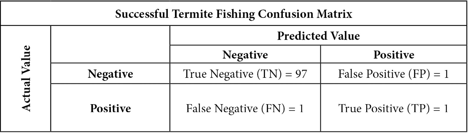
Figure 6.2 – Successful termite fishing confusion matrix

Notice that we get a very high accuracy of 98% – that is, (97+1) / 100. We get high accuracy and low sensitivity because a large percentage of the fishing attempts are negative and that is easy to predict. A model that just predicts failure always would also have an accuracy of 98%.

Now, let’s look at these model evaluation measures with real data. We can experiment with a k-nearest neighbors (KNN) model to predict bachelor’s degree attainment and evaluate its accuracy, sensitivity, specificity, and precision:

1. We will start by loading libraries for encoding and standardizing data, and for creating training and testing DataFrames. We will also load scikit-learn’s KNN classifier and the metrics library:

   import pandas as pd

   import numpy as np

   from feature_engine.encoding import OneHotEncoder

   from sklearn.model_selection import train_test_split

   from sklearn.preprocessing import StandardScaler

   from sklearn.neighbors import KNeighborsClassifier

   import sklearn.metrics as skmet

   import matplotlib.pyplot as plt

2. Now, we can create training and testing DataFrames and encode and scale the data:

   nls97compba = pd.read_csv("data/nls97compba.csv")

   feature_cols = ['satverbal','satmath','gpaoverall',

     'parentincome','gender']

   X_train, X_test, y_train, y_test =  

     train_test_split(nls97compba[feature_cols],

     nls97compba[['completedba']], test_size=0.3, random_state=0)

   ohe = OneHotEncoder(drop_last=True, variables=['gender'])

   ohe.fit(X_train)

   X_train_enc, X_test_enc =

     ohe.transform(X_train), ohe.transform(X_test)

   scaler = StandardScaler()

   standcols = X_train_enc.iloc[:,:-1].columns

   scaler.fit(X_train_enc[standcols])

   X_train_enc =

     pd.DataFrame(scaler.transform(X_train_enc[standcols]),

     columns=standcols, index=X_train_enc.index).

     join(X_train_enc[['gender_Female']])

   X_test_enc =

     pd.DataFrame(scaler.transform(X_test_enc[standcols]),

     columns=standcols, index=X_test_enc.index).

     join(X_test_enc[['gender_Female']])

3. Let’s create a KNN classification model. We will not worry too much about how we specify it since we just want to focus on evaluation measures in this section. We will use all of the features listed in feature_cols We use the predict method of the KNN classifier to generate predictions from the testing data:

   knn = KNeighborsClassifier(n_neighbors = 5)

   knn.fit(X_train_enc, y_train.values.ravel())

   pred = knn.predict(X_test_enc)

4. We can use scikit-learn to plot a confusion matrix. We will pass the actual values in the testing data (y_test) and predicted values to the confusion_matrix method:

   cm = skmet.confusion_matrix(y_test, pred, labels=knn.classes_)

   cmplot = skmet.ConfusionMatrixDisplay(

     confusion_matrix=cm,

     display_labels=['Negative', 'Positive'])

   cmplot.plot()

   cmplot.ax_.set(title='Confusion Matrix',

     xlabel='Predicted Value', ylabel='Actual Value')

This generates the following plot:

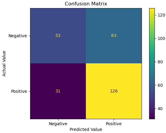
Figure 6.3 – Confusion matrix of actual and predicted values

5. We can also just return the true negative, false positive, false negative, and true positive counts:

   tn, fp, fn, tp = skmet.confusion_matrix(

     y_test.values.ravel(), pred).ravel()

   tn, fp, fn, tp

   (53, 63, 31, 126)

6. We now have what we need to calculate accuracy, sensitivity, specificity, and precision:

   accuracy = (tp + tn) / pred.shape[0]

   accuracy

   0.6556776556776557

   sensitivity = tp / (tp + fn)

   sensitivity

   0.802547770700637

   specificity = tn / (tn+fp)

   specificity

   0.45689655172413796

   precision = tp / (tp + fp)

   precision

   0.6666666666666666

This model has relatively low accuracy, but somewhat better sensitivity; that is, it does a better job of identifying those in the testing data who have completed a bachelor’s degree than of correctly identifying both degree completers and non-completers overall. If we look back at the confusion matrix, we will see that there are a fair number of false positives, as our model predicts that 63 individuals in the testing data would have a bachelor’s degree who did not.

7. We could have also used scikit-learn handy methods for generating these statistics directly:

   skmet.accuracy_score(y_test.values.ravel(), pred)

   0.6556776556776557

   skmet.recall_score(y_test.values.ravel(), pred)

   0.802547770700637

   skmet.precision_score(y_test.values.ravel(), pred)

   0.6666666666666666

Just for comparison, let’s try a random forest classifier and see if we get any better results.

8. Let’s fit a random forest classifier to the same data and call confusion_matrix again:

   rfc = RandomForestClassifier(n_estimators=100,

     max_depth=2, n_jobs=-1, random_state=0)

   rfc.fit(X_train_enc, y_train.values.ravel())

   pred = rfc.predict(X_test_enc)

   tn, fp, fn, tp = skmet.confusion_matrix(

     y_test.values.ravel(), pred).ravel()

   tn, fp, fn, tp

   (49, 67, 17, 140)

   accuracy = (tp + tn) / pred.shape[0]

   accuracy

   0.6923076923076923

   sensitivity = tp / (tp + fn)

   sensitivity

   0.89171974522293

   specificity = tn / (tn+fp)

   specificity

   0.4224137931034483

   precision = tp / (tp + fp)

   precision

   0.6763285024154589

The second model gets us significantly fewer false negatives and more true positives than the first model. It is less likely to predict no bachelor’s degree when individuals in the test data have completed a bachelor’s degree, and more likely to predict a bachelor’s degree when the person has completed one. The main impact of the lower FP and higher TP is a significantly higher sensitivity. The second model identifies actual positives 89% of the time, compared with 80% for the first model.

The measures we have discussed in this section – accuracy, sensitivity, specificity, and precision – are worth looking at whenever we are evaluating a classification model. But it can be hard to get a good sense of the tradeoffs we are sometimes confronted with, between precision and sensitivity, for example. Data scientists rely on several standard visualizations to improve our sense of these tradeoffs when building classification models. We will examine these visualizations in the next section.

Examining CAP, ROC, and precision-sensitivity curves for binary classification

There are several ways to visualize the performance of a binary classification model. A relatively straightforward visualization is the Cumulative Accuracy Profile (CAP), which shows the ability of our model to identify in-class, or positive, cases. It shows the cumulative cases on the X-axis and the cumulative positive outcomes on the Y-axis. A CAP curve is a good way to see how good a job our model does at discriminating in-class observations. (When discussing binary classification models, I will use the terms in-class and positive interchangeably.)

Receiver operating characteristic (ROC) curves illustrate the tradeoff between model sensitivity (being able to identify positive values) and the false positive rate as we adjust the threshold for classifying a positive value. Similarly, precision-sensitivity curves show the relationship between the reliability of our positive predictions (their precision) and sensitivity (our model’s ability to identify positive actual values) as we adjust the threshold.

Constructing CAP curves

Let’s start with CAP curves for our bachelor’s completion KNN model. Let’s also compare that with a decision tree model. Again, we will not do much with feature selection here. The previous chapter went over feature selection in some detail.

In addition to curves for our models, CAP curves also have plots of a random model and a perfect model to view for comparison. The random model provides no information other than the overall distribution of positive values. The perfect model predicts positive values precisely. To illustrate how those plots are drawn, we will start with a hypothetical example. Imagine that you sample the first six cards of a nicely shuffled deck of playing cards. You create a table with the cumulative card total in one column and the number of red cards in the next column. It may look something like this:

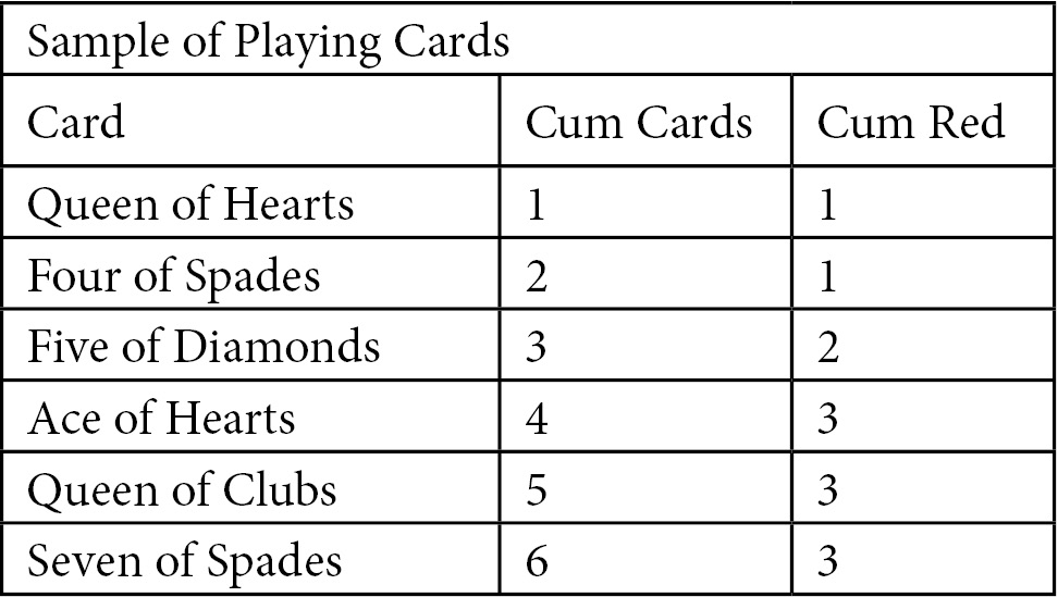
Figure 6.4 – Sample of playing cards

We can plot a random model based on just our knowledge of the number of red cards. The random model has just two points, (0,0) and (6,3), but that is all we need.

The perfect model plot requires a bit more explanation. If our model predicted red cards perfectly and we sorted by the prediction in descending order, we would get Figure 6.5. The cumulative in-class count matches the number of cards until the red cards have been exhausted, which is 3 in this case. A plot of the cumulative in-class total with a perfect model would have two slopes; equal to 1 up until the in-class total was reached, and then 0 after that:

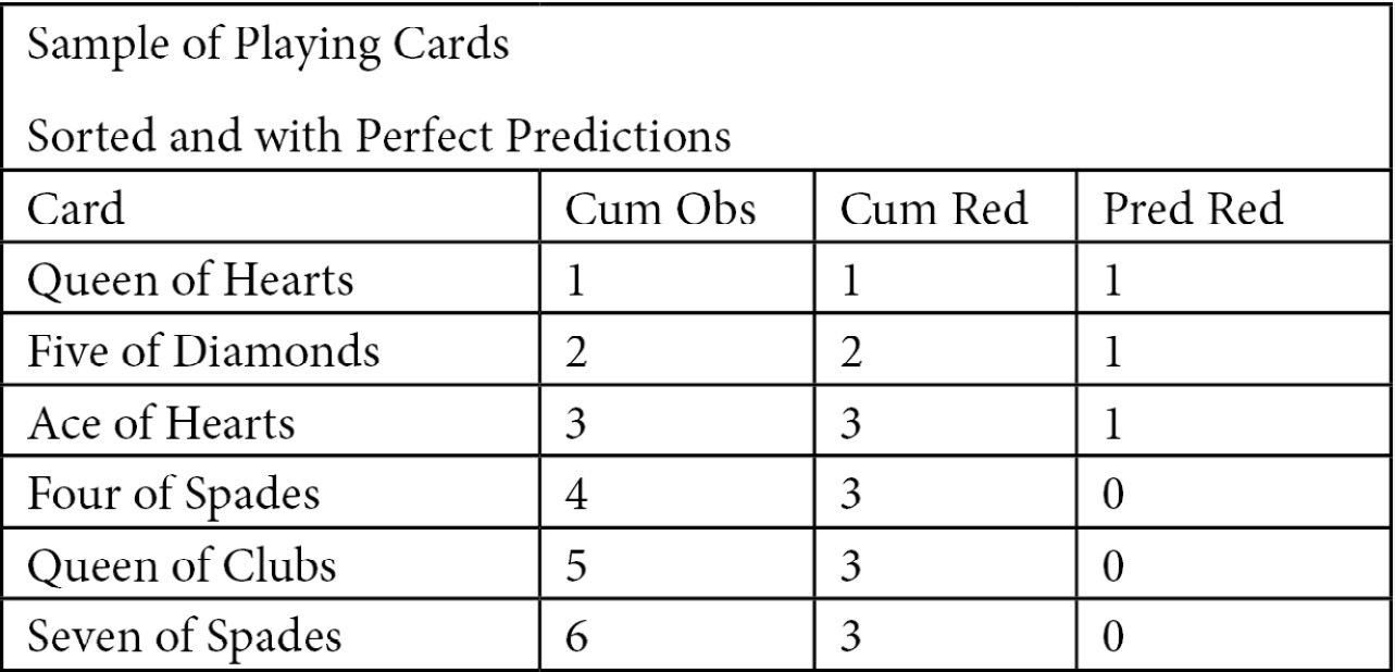
Figure 6.5 – Sample of playing cards

We now know enough to plot both the random model and the perfect model. The perfect model will have three points: (0,0), (in-class count, in-class count), and (number of cards, in-class count). In this case, in-class count is 3 and the number of cards is 6:

numobs = 6

inclasscnt = 3

plt.yticks([1,2,3])

plt.plot([0, numobs], [0, inclasscnt], c = 'b', label = 'Random Model')

plt.plot([0, inclasscnt, numobs], [0, inclasscnt, inclasscnt], c = 'grey', linewidth = 2, label = 'Perfect Model')

plt.title("Cumulative Accuracy Profile")

plt.xlabel("Total Cards")

plt.ylabel("In-class (Red) Cards")

This produces the following plot:

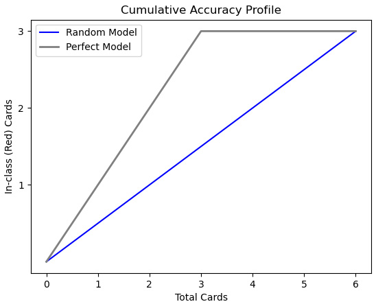
Figure 6.6 – CAP with playing card data

One way to understand the improvement of the perfect model over the random model is to consider how many red cards the random model would predict at the midpoint – that is, 3 cards. At that point, the random model would predict 1.5 red cards. However, the perfect model would predict 3. (Remember that we have sorted the cards by prediction in descending order.)

Having constructed plots for random and perfect models with made-up data, let’s try it with our bachelor’s degree completion data:

1. First, we must import the same modules as in the previous section:

   import pandas as pd

   import numpy as np

   from feature_engine.encoding import OneHotEncoder

   from sklearn.model_selection import train_test_split

   from sklearn.preprocessing import StandardScaler

   from sklearn.neighbors import KNeighborsClassifier

   from sklearn.ensemble import RandomForestClassifier

   import sklearn.metrics as skmet

   import matplotlib.pyplot as plt

   import seaborn as sb

2. Then, we load, encode, and scale the NLS bachelor’s degree data:

   nls97compba = pd.read_csv("data/nls97compba.csv")

   feature_cols = ['satverbal','satmath','gpaoverall',

     'parentincome','gender']

   X_train, X_test, y_train, y_test =  

     train_test_split(nls97compba[feature_cols],

     nls97compba[['completedba']], test_size=0.3, random_state=0)

   ohe = OneHotEncoder(drop_last=True, variables=['gender'])

   ohe.fit(X_train)

   X_train_enc, X_test_enc =

     ohe.transform(X_train), ohe.transform(X_test)

   scaler = StandardScaler()

   standcols = X_train_enc.iloc[:,:-1].columns

   scaler.fit(X_train_enc[standcols])

   X_train_enc =

     pd.DataFrame(scaler.transform(X_train_enc[standcols]),

     columns=standcols, index=X_train_enc.index).

     join(X_train_enc[['gender_Female']])

   X_test_enc =

     pd.DataFrame(scaler.transform(X_test_enc[standcols]),

     columns=standcols, index=X_test_enc.index).

     join(X_test_enc[['gender_Female']])

3. Next, we create KNeighborsClassifier and RandomForestClassifier instances:

   knn = KNeighborsClassifier(n_neighbors = 5)

   rfc = RandomForestClassifier(n_estimators=100, max_depth=2,

     n_jobs=-1, random_state=0)

We are now ready to start plotting our CAP curves. We will start by drawing a random model and then a perfect model. These are models that use no information (other than the overall distribution of positive values) and that provide perfect information, respectively.

4. We count the number of observations in the test data and the number of positive values. We will use (0,0) and (the number of observations, in-class count) to draw the random model line. For the perfect model, we will plot a line from (0,0) to (in-class count, in-class count) since that model can perfectly discriminate in-class values (it is never wrong). It is flat to the right of that point since there are no more positive values to find.

We will also draw a vertical line at the midpoint and a horizontal line where that intersects the random model line. This will be more useful later:

numobs = y_test.shape[0]

inclasscnt = y_test.iloc[:,0].sum()

plt.plot([0, numobs], [0, inclasscnt], c = 'b', label = 'Random Model')

plt.plot([0, inclasscnt, numobs], [0, inclasscnt, inclasscnt], c = 'grey', linewidth = 2, label = 'Perfect Model')

plt.axvline(numobs/2, color='black', linestyle='dashed', linewidth=1)

plt.axhline(numobs/2, color='black', linestyle='dashed', linewidth=1)

plt.title("Cumulative Accuracy Profile")

plt.xlabel("Total Observations")

plt.ylabel("In-class Observations")

plt.legend()

This produces the following plot:

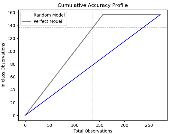
Figure 6.7 – CAP with just random and perfect models

5. Next, we define a function to plot a CAP curve for a model we pass to it. We will use the predict_proba method to get an array with the probability that each observation in the test data is in-class (in this case, has completed a bachelor’s degree). Then, we will create a DataFrame with those probabilities and the actual target value, sort it by probability in reverse order, and calculate a running total of positive actual target values.

We will also get the value of the running total at the middle observation and draw a horizontal line at that point. Finally, we will plot a line that has an array from 0 to the number of observations as x values, and the running in-class totals as y values:

def addplot(model, X, Xtest, y, modelname, linecolor):

  model.fit(X, y.values.ravel())

  probs = model.predict_proba(Xtest)[:, 1]

  probdf = pd.DataFrame(zip(probs, y_test.values.ravel()),

    columns=(['prob','inclass']))

  probdf.loc[-1] = [0,0]

  probdf = probdf.sort_values(['prob','inclass'],

    ascending=False).

    assign(inclasscum = lambda x: x.inclass.cumsum())

  inclassmidpoint =

    probdf.iloc[int(probdf.shape[0]/2)].inclasscum

  plt.axhline(inclassmidpoint, color=linecolor,

    linestyle='dashed', linewidth=1)

  plt.plot(np.arange(0, probdf.shape[0]),

    probdf.inclasscum, c = linecolor,

    label = modelname, linewidth = 4)

6. Now, let’s run the function for the KNN and random forest classifier models using the same data:

   addplot(knn, X_train_enc, X_test_enc, y_train,

     'KNN', 'red')

   addplot(rfc, X_train_enc, X_test_enc, y_train,

     'Random Forest', 'green')

   plt.legend()

This updates our earlier plot:

Figure 6.8 – CAP updated with KNN and random forest models

Not surprisingly, the CAP curves show that our KNN and random forest models are better than randomly guessing, but not as good as a perfect model. The question is, how much better and how much worse, respectively. The horizontal lines give us some idea. A perfect model would have correctly identified 138 positive values out of 138 observations. (Recall that the observations are sorted so that the observations with the highest likelihood of being positive are first.) The random model would have identified 70 (line not shown), while the KNN and random forest models would have identified 102 and 103, respectively. Our two models are 74% and 75% as good as a perfect model would have been at discriminating positive values. Anything between 70% and 80% is considered to be a good model; percentages above that are very good, while percentages below that are poor.

Plotting a receiver operating characteristic (ROC) curve

ROC curves illustrate the tradeoff between the false positive rate and the true positive rate (also known as sensitivity) as we adjust the threshold. We should discuss the false positive rate before going further. It is the percentage of actual negatives (true negatives plus false positives) that our model falsely identifies as positive:

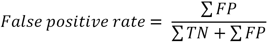
Here, you can see the relationship that the false positive rate has with specificity, which was discussed at the beginning of this chapter. The difference is the numerator. Specificity is the percentage of actual negatives that our model correctly identifies as negative:

We can also compare the false positive rate with sensitivity, which is the percentage of actual positives (true positives plus false negatives) that our model correctly identifies as positive:

We are typically confronted with a tradeoff between sensitivity and the false positive rate. We want our models to be able to identify a large percentage of the actual positives, but we do not want a problematically high false positive rate. What is problematically high depends on your context.

The tradeoff between sensitivity and the false positive rate is trickier the more difficult it is to discriminate between negative and positive cases. We can see this with our bachelor’s degree completion model when we plot the predicted probabilities:

1. First, let’s fit our random forest classifier again and generate predictions and prediction probabilities. We will see that this model predicts that the person completes a bachelor’s degree when the predicted probability is greater than 0.500:

   rfc.fit(X_train_enc, y_train.values.ravel())

   pred = rfc.predict(X_test_enc)

   pred_probs = rfc.predict_proba(X_test_enc)[:, 1]

   probdf = pd.DataFrame(zip(

     pred_probs, pred, y_test.values.ravel()),

     columns=(['prob','pred','actual']))

   probdf.groupby(['pred'])['prob'].agg(['min','max'])

                   min             max

   pred             

   0.000           0.305           0.500

   1.000           0.502           0.883

2. It is helpful to compare the distribution of these probabilities with the actual class values. We can do this with density plots:

   sb.kdeplot(probdf.loc[probdf.actual==1].prob,

     shade=True, color='red',

     label="Completed BA")

   sb.kdeplot(probdf.loc[probdf.actual==0].prob,  

     shade=True, color='green',

     label="Did Not Complete")

   plt.axvline(0.5, color='black', linestyle='dashed', linewidth=1)

   plt.axvline(0.65, color='black', linestyle='dashed', linewidth=1)

   plt.title("Predicted Probability Distribution")

   plt.legend(loc="upper left")

This produces the following plot:

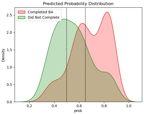
Figure 6.9 – Density plot of in-class and out-of-class observations

Here, we can see that our model has some trouble discriminating between actual positive and negative values since there is a fair bit of in-class and out-of-class overlap. A threshold of 0.500 (the left dotted line) gets us a lot of false positives since a good portion of the distribution of out-of-class observations (those not completing bachelor’s degrees) have predicted probabilities greater than 0.500. If we move the threshold higher, say to 0.650, we get many more false negatives since many in-class observations have probabilities lower than 0.65.

3. It is easy to construct a ROC curve based on the testing data and the random forest model. The roc_curve method returns both the false positive rate (fpr) and sensitivity (true positive rate, tpr) at different thresholds (ths).

First, let’s draw separate false positive rate and sensitivity lines by threshold:

fpr, tpr, ths = skmet.roc_curve(y_test, pred_probs)

ths = ths[1:]

fpr = fpr[1:]

tpr = tpr[1:]

fig, ax = plt.subplots()

ax.plot(ths, fpr, label="False Positive Rate")

ax.plot(ths, tpr, label="Sensitivity")

ax.set_title('False Positive Rate and Sensitivity by Threshold')

ax.set_xlabel('Threshold')

ax.set_ylabel('False Positive Rate and Sensitivity')

ax.legend()

This produces the following plot:

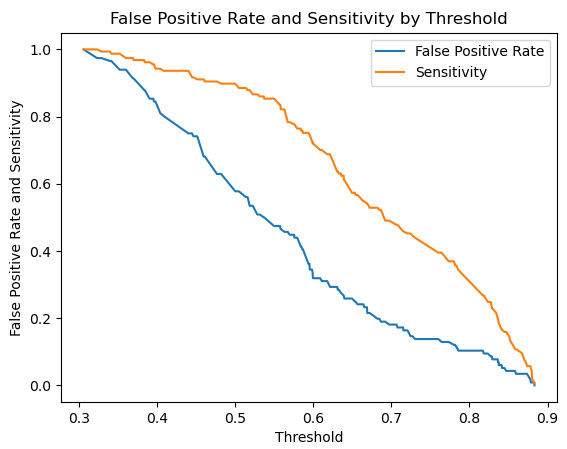
Figure 6.10 – False positive rate and sensitivity lines

Here, we can see that increasing the threshold will improve (reduce) our false positive rate, but also lower our sensitivity.

4. Now, let’s draw the associated ROC curve, which plots the false positive rate against sensitivity for each threshold:

   fig, ax = plt.subplots()

   ax.plot(fpr, tpr, linewidth=4, color="black")

   ax.set_title('ROC curve')

   ax.set_xlabel('False Positive Rate')

   ax.set_ylabel('Sensitivity')

This produces the following plot:

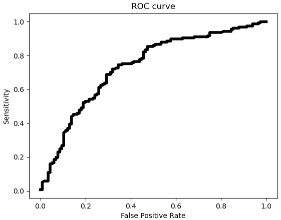
Figure 6.11 – ROC curve with false positive rate and sensitivity

The ROC curve indicates that the tradeoff between the false positive rate and sensitivity is pretty steep until the false positive rate is about 0.5 or higher. Let’s see what that means for the threshold of 0.5 that was used for the random forest model predictions.

5. Let’s select an index from the threshold array that is near 0.5, and also one near 0.4 and 0.6 for comparison. Then, we will draw vertical lines for the false positive rate at those indexes, and horizontal lines for the sensitivity values at those indexes:

   tholdind = np.where((ths>0.499) & (ths<0.501))[0][0]

   tholdindlow = np.where((ths>0.397) & (ths<0.404))[0][0]

   tholdindhigh = np.where((ths>0.599) & (ths<0.601))[0][0]

   plt.vlines((fpr[tholdindlow],fpr[tholdind],

     fpr[tholdindhigh]), 0, 1, linestyles ="dashed",

     colors =["green","blue","purple"])

   plt.hlines((tpr[tholdindlow],tpr[tholdind],

     tpr[tholdindhigh]), 0, 1, linestyles ="dashed",

     colors =["green","blue","purple"])

This updates our plot:

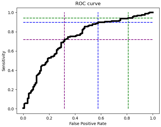
Figure 6.12 – ROC curve with lines for thresholds

This illustrates the tradeoff between the false positive rate and sensitivity at the 0.5 threshold (the blue dashed line) used for predictions. The ROC curve has very little slope with thresholds above 0.5, such as with the 0.6 threshold (the green dashed line). So, reducing the threshold from 0.6 to 0.5 results in a substantially lower false positive rate (from above 0.8 to below 0.6), but not much reduction in sensitivity. However, improving (reducing) the false positive rate by reducing the threshold from 0.5 to 0.4 (from the blue to the purple line) leads to significantly worse sensitivity. It drops from nearly 90% to just above 70%.

Plotting precision-sensitivity curves

It is often helpful to examine the relationship between precision and sensitivity as the threshold is adjusted. Remember that precision tells us the percentage of the time we are correct when we predict a positive value:

We can improve precision by increasing the threshold for classifying a value as positive. However, this will likely mean a reduction in sensitivity. As we improve how often we are correct when we predict a positive value (precision), we will decrease the number of positive values we are able to identify (sensitivity). Precision-sensitivity curves, often called precision-recall curves, illustrate this tradeoff.

Before drawing the precision-sensitivity curve, let’s look at separate precision and sensitivity lines plotted against thresholds:

1. We can get the points for the precision-sensitivity curves with the precision_recall_curve method. We remove some squirreliness at the highest threshold values, which can sometimes happen:

   prec, sens, ths = skmet.precision_recall_curve(y_test, pred_probs)

   prec = prec[1:-10]

   sens = sens[1:-10]

   ths  = ths[:-10]

   fig, ax = plt.subplots()

   ax.plot(ths, prec, label='Precision')

   ax.plot(ths, sens, label='Sensitivity')

   ax.set_title('Precision and Sensitivity by Threshold')

   ax.set_xlabel('Threshold')

   ax.set_ylabel('Precision and Sensitivity')

   ax.set_xlim(0.3,0.9)

   ax.legend()

This produces the following plot:

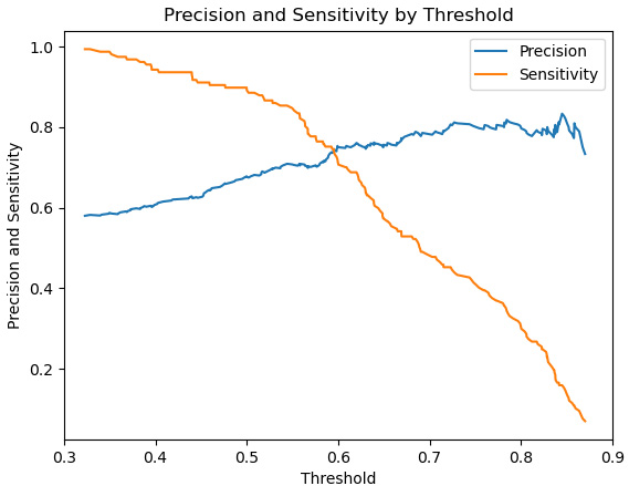
Figure 6.13 – Precision and sensitivity lines

Here, we can see that sensitivity declines more steeply with thresholds above 0.5. This decline does not buy us much improved precision beyond the 0.6 threshold.

2. Now, let’s plot sensitivity against precision to view the precision-sensitivity curve:

   fig, ax = plt.subplots()

   ax.plot(sens, prec)

   ax.set_title('Precision-Sensitivity Curve')

   ax.set_xlabel('Sensitivity')

   ax.set_ylabel('Precision')

   plt.yticks(np.arange(0.2, 0.9, 0.2))

This produces the following plot:

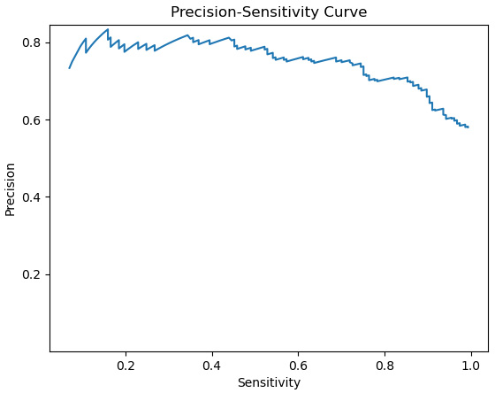
Figure 6.14 – Precision-sensitivity curve

The precision-sensitivity curve reflects the fact that sensitivity is much more responsive to threshold than is precision with this particular model. This means that we could decrease the threshold below 0.5 to get greater sensitivity, without a significant reduction in precision.

Note

The choice of threshold is partly a matter of judgment and domain knowledge, and is mostly an issue when we have significant class imbalance. However, in Chapter 10, Logistic Regression we will explore how to calculate an optimal threshold.

This section, and the previous one, demonstrated how to evaluate binary classification models. They showed that model evaluation is not just a thumbs up and thumbs down process. It is much more like tasting your batter as you make a cake. We make good initial assumptions about our model specification and use the model evaluation process to make improvements. This often involves tradeoffs between accuracy, sensitivity, specificity, and precision, and modeling decisions that resist one-size-fits-all recommendations. These decisions are very much domain-dependent and a matter of professional judgment.

The discussion in this section, and most of the techniques, apply as much to multiclass modeling. We discuss evaluating multiclass models in the next section.

Evaluating multiclass models

All of the same principles that we used to evaluate binary classification models apply to multiclass model evaluation. Computing a confusion matrix is just as important, though a fair bit more difficult to interpret. We also still need to examine somewhat competing measures, such as precision and sensitivity. This, too, is messier than doing so with binary classification.

Once again, we will work with the NLS degree completion data. We will alter the target in this case, from bachelor’s degree completion or not to high school completion, bachelor’s degree completion, and post-graduate degree completion:

1. We will start by loading the necessary libraries. These are the same libraries we used in the previous two sections:

   import pandas as pd

   import numpy as np

   from feature_engine.encoding import OneHotEncoder

   from sklearn.model_selection import train_test_split

   from sklearn.preprocessing import StandardScaler

   from sklearn.neighbors import KNeighborsClassifier

   import sklearn.metrics as skmet

   import matplotlib.pyplot as plt

2. Next, we will load the NLS degree attainment data, create training and testing DataFrames, and encode and scale the data:

   nls97degreelevel = pd.read_csv("data/nls97degreelevel.csv")

   feature_cols = ['satverbal','satmath','gpaoverall',

     'parentincome','gender']

   X_train, X_test, y_train, y_test =  

     train_test_split(nls97degreelevel[feature_cols],

     nls97degreelevel[['degreelevel']], test_size=0.3, random_state=0)

   ohe = OneHotEncoder(drop_last=True, variables=['gender'])

   ohe.fit(X_train)

   X_train_enc, X_test_enc =

     ohe.transform(X_train), ohe.transform(X_test)

   scaler = StandardScaler()

   standcols = X_train_enc.iloc[:,:-1].columns

   scaler.fit(X_train_enc[standcols])

   X_train_enc =

     pd.DataFrame(scaler.transform(X_train_enc[standcols]),

     columns=standcols, index=X_train_enc.index).

     join(X_train_enc[['gender_Female']])

   X_test_enc =

     pd.DataFrame(scaler.transform(X_test_enc[standcols]),

     columns=standcols, index=X_test_enc.index).

     join(X_test_enc[['gender_Female']])

3. Now, we will run a KNN model and predict values for each degree level category:

   knn = KNeighborsClassifier(n_neighbors = 5)

   knn.fit(X_train_enc, y_train.values.ravel())

   pred = knn.predict(X_test_enc)

   pred_probs = knn.predict_proba(X_test_enc)[:, 1]

4. We can use those predictions to generate a confusion matrix:

   cm = skmet.confusion_matrix(y_test, pred)

   cmplot = skmet.ConfusionMatrixDisplay(confusion_matrix=cm, display_labels=['High School', 'Bachelor','Post-Graduate'])

   cmplot.plot()

   cmplot.ax_.set(title='Confusion Matrix',

     xlabel='Predicted Value', ylabel='Actual Value')

This generates the following plot:

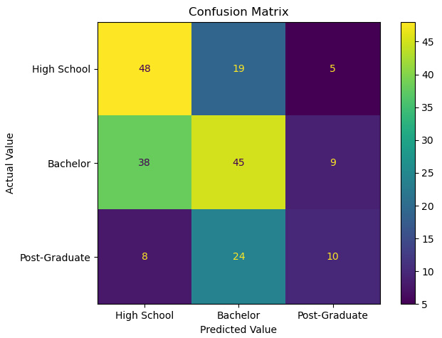
Figure 6.15 – Confusion matrix with a multiclass target

It is possible to calculate evaluation measures by hand. Precision is the percentage of our in-class predictions that are actually in-class. So, for our prediction of high school, it is 48 / (48 + 38 + 8) = 0.51. Sensitivity for the high school class – that is, the percentage of actual values of high school that our model predicts – is 48 / (48 + 19 +5) = 0.67. However, this is fairly tedious. Fortunately, scikit-learn can do this for us.

5. We can call the classification_report method to get these statistics, passing actual and predicted values (remember that recall and sensitivity are the same measure):

   print(skmet.classification_report(y_test, pred,

     target_names=['High School', 'Bachelor', 'Post-Graduate']))

                  precision    recall  f1-score   support

     High School       0.51      0.67      0.58        72

        Bachelor       0.51      0.49      0.50        92

   Post-Graduate       0.42      0.24      0.30        42

        accuracy                           0.50       206

       macro avg       0.48      0.46      0.46       206

   weighted avg       0.49      0.50      0.49       206

In addition to precision and sensitivity rates by class, we get some other statistics. The F1-score is the harmonic mean of precision and sensitivity.

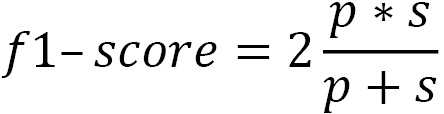
Here, p is precision and s is sensitivity.

To get the average precision, sensitivity, and F1-score across classes, we can either use the simple average (macro average) or a weighted average that adjusts for class size. Using the weighted average, we get precision, sensitivity, and F1-score values of 0.49, 0.50, and 0.49, respectively. (Since the classes are relatively balanced here, there is not much difference between the macro average and the weighted average.)

This demonstrates how to extend the evaluation measures we discussed for binary classification models to multiclass evaluation. The same concepts and techniques apply, though they are more difficult to implement.

So far, we have focused on metrics and visualizations to help us evaluate classification models. We have not examined metrics for evaluating regression models yet. These metrics can be somewhat more straightforward than those for classification. We will discuss them in the next section.

Evaluating regression models

Metrics for regression evaluation are typically based on the distance between the actual values for the target variable and a model’s predicted values. The most common measures – mean squared error, root mean squared error, mean absolute error, and R-squared – all track how successfully our predictions capture variation in a target.

The distance between the actual value and our prediction is known as the residual, or error. The mean squared error (MSE) is the mean of the square of the residuals:

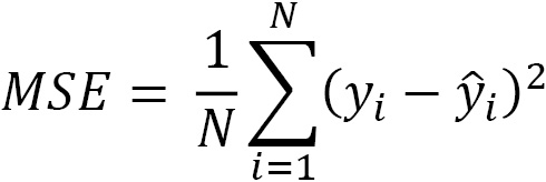
Here, is the actual target variable value at the ith observation and is our prediction for the target. The residuals are squared to handle negative values, where the predicted value is higher than the actual value. To return our measurement to a more meaningful scale, we often use the square root of MSE. That is known as root mean squared error (RMSE).

Due to the squaring, MSE will penalize larger residuals much more than it will smaller residuals. For example, if we have predictions for five observations, with one having a residual of 25, and the other four having a residual of 0, we will get an MSE of (0+0+0+0+625)/5 = 125. However, if all five observations had residuals of 5, the MSE would be (25+25+25+25+25)/5 = 25.

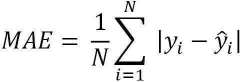
A good alternative to squaring the residuals is to take their absolute value. This gives us the mean absolute error:

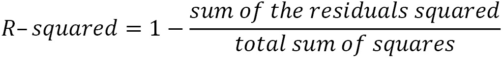
R-squared, also known as the coefficient of determination, is an estimate of the proportion of the variation in the target variable captured by our model. We square the residuals, as we do when calculating MSE, and divide that by the deviation of each actual target value from its sample mean. This gives us the still unexplained variation, which we subtract from 1 to get the explained variation:

Fortunately, scikit-learn makes it easy to generate these statistics. In this section, we will build a linear regression model of land temperatures and use these statistics to evaluate it. We will work with data from the United States National Oceanic and Atmospheric Administration on average annual temperatures, elevation, and latitude at weather stations in 2019.

Note

The land temperature dataset contains the average temperature readings (in Celsius) in 2019 from over 12,000 stations across the world, though the majority of the stations are in the United States. The raw data was retrieved from the Global Historical Climatology Network integrated database. It has been made available for public use by the United States National Oceanic and Atmospheric Administration at https://www.ncdc.noaa.gov/data-access/land-based-station-data/land-based-datasets/global-historical-climatology-network-monthly-version-4.

Let’s start building a linear regression model:

1. We will start by loading the libraries we need and the land temperatures data. We will also create training and testing DataFrames:

   import pandas as pd

   import numpy as np

   from sklearn.model_selection import train_test_split

   from sklearn.linear_model import LinearRegression

   import sklearn.metrics as skmet

   import matplotlib.pyplot as plt

   landtemps = pd.read_csv("data/landtemps2019avgs.csv")

   feature_cols = ['latabs','elevation']

   X_train, X_test, y_train, y_test =  

     train_test_split(landtemps[feature_cols],

     landtemps[['avgtemp']], test_size=0.3, random_state=0)

   Note

   The latabs feature is the value of latitude without the North or South indicators; so, Cairo, Egypt, at approximately 30 degrees north, and Porto Alegre, Brazil, at about 30 degrees south, have the same value.

2. Now, we scale our data:

   scaler = StandardScaler()

   scaler.fit(X_train)

   X_train =

     pd.DataFrame(scaler.transform(X_train),

     columns=feature_cols, index=X_train.index)

   X_test =

     pd.DataFrame(scaler.transform(X_test),

     columns=feature_cols, index=X_test.index)

   scaler.fit(y_train)

   y_train, y_test =

     pd.DataFrame(scaler.transform(y_train),

     columns=['avgtemp'], index=y_train.index),

     pd.DataFrame(scaler.transform(y_test),

     columns=['avgtemp'], index=y_test.index)

3. Next, we instantiate a scikit-learn LinearRegression object and fit a model on the training data. Our target is the annual average temperature (avgtemp), while the features are latitude (latabs) and elevation. The coef_ attribute gives us the coefficient for each feature:

   lr = LinearRegression()

   lr.fit(X_train, y_train)

   np.column_stack((lr.coef_.ravel(),

     X_test.columns.values))

   array([[-0.8538957537748768, 'latabs'],

          [-0.3058979822791853, 'elevation']], dtype=object)

The interpretation of the latabs coefficient is that standardized average annual temperature will decline by 0.85 for every one standard deviation increase in latitude. (The LinearRegression module does not return p-values, a measure of the statistical significance of the coefficient estimate. You can use statsmodels instead to see a full summary of an ordinary least squares model.)

4. Now, we can get predicted values. Let’s also join the returned NumPy array with the features and the target from the testing data. Then, we can calculate the residuals by subtracting the predicted values from the actual values (avgtemp). The residuals do not look bad, though there is a little negative skew and excessive kurtosis:

   pred = lr.predict(X_test)

   preddf = pd.DataFrame(pred, columns=['prediction'],

     index=X_test.index).join(X_test).join(y_test)

   preddf['resid'] = preddf.avgtemp-preddf.prediction

   preddf.resid.agg(['mean','median','skew','kurtosis'])

   mean             -0.021

   median           0.032

   skew              -0.641

   kurtosis        6.816

   Name: resid, dtype: float64

It is worth noting that we will be generating predictions and calculated residuals in this way most of the time we work with regression models in this book. If you feel a little unclear about what we just did in the preceding code block, it may be a good idea to go over it again.

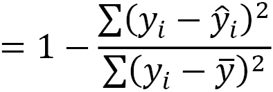
5. We should plot the residuals to get a better sense of how they are distributed.

   Plt.hist(preddf.resid, color="blue")

   plt.axvline(preddf.resid.mean(), color='red', linestyle='dashed', linewidth=1)

   plt.title("Histogram of Residuals for Temperature Model")

   plt.xlabel("Residuals")

   plt.ylabel("Frequency")

This produces the following plot:

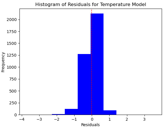
Figure 6.16 – Histogram of residuals for the linear regression model

This does not look too bad, but we have more positive residuals, where we have predicted a lower temperature in the testing data than the actual temperature, than negative residuals.

6. Plotting our predictions by the residuals may give us a better sense of what is happening:

   plt.scatter(preddf.prediction, preddf.resid, color="blue")

   plt.axhline(0, color='red', linestyle='dashed', linewidth=1)

   plt.title("Scatterplot of Predictions and Residuals")

   plt.xlabel("Predicted Temperature")

   plt.ylabel("Residuals")

This produces the following plot:

Figure 6.17 – Scatterplot of predictions by residuals for the linear regression model

This does not look horrible. The residuals hover somewhat randomly around 0. However, predictions between 1 and 2 standard deviations are much more likely to be too low (to have positive residuals) than too high. Above 2, the predictions are always too high (they have negative residuals). This model’s assumption of linearity might not be sound. We should explore a couple of the transformations we discussed in Chapter 4, Encoding, Transforming, and Scaling Features, or try a non-parametric model such as KNN regression.

It is also likely that extreme values are tugging our coefficients around a fair bit. A good next move might be to remove outliers, as we discussed in the Identifying extreme values and outliers section of Chapter 1, Examining the Distribution of Features and Targets. We will not do that here, however.

7. Let’s look at some evaluation measures. This can easily be done with scikit-learn’s metrics library. We can call the same function to get RMSE as MSE. We just need to set the squared parameter to False:

   mse = skmet.mean_squared_error(y_test, pred)

   mse

   0.18906346144036693

   rmse = skmet.mean_squared_error(y_test, pred, squared=False)

   rmse

   0.4348142838504353

   mae = skmet.mean_absolute_error(y_test, pred)

   mae

   0.318307379728143

   r2 = skmet.r2_score(y_test, pred)

   r2

   0.8162525715296725

An MSE of less than 0.2 of a standard deviation and an MAE of less than 0. 3 of a standard deviation look pretty decent, especially for such a sparse model. An R-squared above 80% is also fairly promising.

8. Let’s see what we get if we use a KNN model instead:

   knn = KNeighborsRegressor(n_neighbors=5)

   knn.fit(X_train, y_train)

   pred = knn.predict(X_test)

   mae = skmet.mean_absolute_error(y_test, pred)

   mae

   0.2501829988751876

   r2 = skmet.r2_score(y_test, pred)

   r2

   0.8631113217183314

This model is actually an improvement in both MAE and R-squared.

9. We should also take a look at the residuals again:

   preddf = pd.DataFrame(pred, columns=['prediction'],

     index=X_test.index).join(X_test).join(y_test)

   preddf['resid'] = preddf.avgtemp-preddf.prediction

   plt.scatter(preddf.prediction, preddf.resid, color="blue")

   plt.axhline(0, color='red', linestyle='dashed', linewidth=1)

   plt.title("Scatterplot of Predictions and Residuals with KNN Model")

   plt.xlabel("Predicted Temperature")

   plt.ylabel("Residuals")

   plt.show()

This produces the following plot:

Figure 6.18 – Scatterplot of predictions by residuals for the KNN model

This plot of the residuals looks better as well. There are no parts of the target’s distribution where we are much more likely to over-predict or under-predict.

This section has introduced key measures for evaluating regression models, and how to interpret them. It has also demonstrated how visualizations, particularly of model residuals, can improve that interpretation.

However, we have been limited so far, in both our use of regression and classification measures, by how we have constructed our training and testing DataFrames. What if, for some reason, the testing data is unusual in some way? More generally, what is our basis for concluding that our evaluation measures are accurate? We can be more confident in these measures if we use K-fold cross-validation, which we will cover in the next section.

Using K-fold cross-validation

So far, we have held back 30% of our data for validation. This is not a bad strategy. It prevents us from peeking ahead to the testing data as we train our model. However, this approach does not take full advantage of all the available data, either for training or for testing. If we use K-fold cross-validation instead, we can use all of our data while also avoiding data leakage. Perhaps that seems too good to be true. But it’s not because of a neat little trick.

K-fold cross-validation trains our model on all but one of the K folds, or parts, leaving one out for testing. This is repeated k times, each time excluding a different fold for testing. Performance metrics are then based on the average scores across the K folds.

Before we start, though, we need to think again about the possibility of data leakage. If we scale all of the data that we will use to train our model and then split it up into folds, we will be using information from all the folds in our training. To avoid this, we need to do the scaling, as well as any other Preprocessing, on just the training folds for each iteration. While we could do this manually, scikit-learn’s pipeline library can do much of this work for us. We will go over how to use pipelines for cross-validation in this section.

Let’s try evaluating the two models we specified in the previous section using K-fold cross-validation. While we are at it, let’s also see how well a random forest regressor may work:

1. In addition to the libraries we have worked with so far, we need scikit-learn’s make_pipeline, cross_validate, and Kfold libraries:

   import pandas as pd

   from sklearn.model_selection import train_test_split

   from sklearn.preprocessing import StandardScaler

   from sklearn.linear_model import LinearRegression

   from sklearn.neighbors import KNeighborsRegressor

   from sklearn.ensemble import RandomForestRegressor

   from sklearn.pipeline import make_pipeline

   from sklearn.model_selection import cross_validate

   from sklearn.model_selection import KFold

2. We load the land temperatures data again and create training and testing DataFrames. We still want to leave some data out for final validation, but this time, we will only leave out 10%. We will do both training and testing with the remaining 90%:

   landtemps = pd.read_csv("data/landtemps2019avgs.csv")

   feature_cols = ['latabs','elevation']

   X_train, X_test, y_train, y_test =  

     train_test_split(landtemps[feature_cols],

     landtemps[['avgtemp']],test_size=0.1,random_state=0)

3. Now, we create a KFold object and indicate that we want five folds and for the data to be shuffled (shuffling the data is a good idea if it is not already sorted randomly):

   kf = Kfold(n_splits=5, shuffle=True, random_state=0)

4. Next, we define a function to create a pipeline. The function then runs cross_validate, which takes the pipeline and the KFold object we created earlier:

   def getscores(model):

     pipeline = make_pipeline(StandardScaler(), model)

     scores = cross_validate(pipeline, X=X_train,

       y=y_train, cv=kf, scoring=['r2'], n_jobs=1)

     scorelist.append(dict(model=str(model),

       fit_time=scores['fit_time'].mean(),

       r2=scores['test_r2'].mean()))

5. Now, we are ready to call the getscores function for the linear regression, random forest regression, and KNN regression models:

   scorelist = []

   getscores(LinearRegression())

   getscores(RandomForestRegressor(max_depth=2))

   getscores(KNeighborsRegressor(n_neighbors=5))

6. We can print the scorelist list to see our results:

   scorelist

   [{'model': 'LinearRegression()',

     'fit_time': 0.004968833923339844,

     'r2': 0.8181125031214872},

   {'model': 'RandomForestRegressor(max_depth=2)',

     'fit_time': 0.28124608993530276,

     'r2': 0.7122492698889024},

   {'model': 'KNeighborsRegressor()',

     'fit_time': 0.006945991516113281,

     'r2': 0.8686733636724104}]

The KNN regressor model performs better than either the linear regression or random forest regression model, based on R-squared. The random forest regressor also has a significant disadvantage in that it has a much longer fit time.

Preprocessing data with pipelines

We just scratched the surface of what we can do with scikit-learn pipelines in the previous section. We often need to fold all of our Preprocessing and feature engineering into a pipeline, including scaling, encoding, and handling outliers and missing values. This can be complicated as different features may need to be handled differently. We may need to impute the median for missing values with numeric features and the most frequent value for categorical features. We may also need to transform our target variable. We will explore how to do that in this section.

Follow these steps:

1. We will start by loading the libraries we have already worked with in this chapter. Then, we will add the ColumnTransformer and TransformedTargetRegressor classes. We will use those classes to transform our features and target, respectively:

   import pandas as pd

   import numpy as np

   from sklearn.model_selection import train_test_split

   from sklearn.preprocessing import StandardScaler

   from sklearn.linear_model import LinearRegression

   from sklearn.impute import SimpleImputer

   from sklearn.pipeline import make_pipeline

   from feature_engine.encoding import OneHotEncoder

   from sklearn.impute import KNNImputer

   from sklearn.model_selection import cross_validate, KFold

   import sklearn.metrics as skmet

   from sklearn.compose import ColumnTransformer

   from sklearn.compose import TransformedTargetRegressor

2. The column transformer is quite flexible. We can even use it with the Preprocessing functions that we have defined ourselves. The following code block imports the OutlierTrans class from the preprocfunc module in the helperfunctions subfolder:

   import os

   import sys

   sys.path.append(os.getcwd() + "/helperfunctions")

   from preprocfunc import OutlierTrans

3. The OutlierTrans class identifies extreme values by distance from the interquartile range. This is a technique we demonstrated in Chapter 3, Identifying and Fixing Missing Values.

To work in a scikit-learn pipeline, our class has to have fit and transform methods. We also need to inherit the BaseEstimator and TransformerMixin classes.

In this class, almost all of the action happens in the transform method. Any value that is more than 1.5 times the interquartile range above the third quartile or below the first quartile is assigned missing:

class OutlierTrans(BaseEstimator,TransformerMixin):

  def __init__(self,threshold=1.5):

    self.threshold = threshold

  def fit(self,X,y=None):

    return self

  def transform(self,X,y=None):

    Xnew = X.copy()

    for col in Xnew.columns:

      thirdq, firstq = Xnew[col].quantile(0.75),

        Xnew[col].quantile(0.25)

      inlierrange = self.threshold*(thirdq-firstq)

      outlierhigh, outlierlow = inlierrange+thirdq,

        firstq-inlierrange

      Xnew.loc[(Xnew[col]>outlierhigh) |

        (Xnew[col]<outlierlow),col] = np.nan

    return Xnew.values                                 

Our OutlierTrans class can be used later in our pipeline in the same way we used StandardScaler in the previous section. We will do that later.

4. Now, we are ready to load the data that needs to be processed. We will work with the NLS weekly wage data in this section. Weekly wages will be our target, and we will use high school GPA, mother’s and father’s highest grade completed, parent income, gender, and whether the individual completed a bachelor’s degree as features.

We will create lists of features to handle in different ways here. This will be helpful later when we instruct our pipeline to carry out different operations on numerical, categorical, and binary features:

nls97wages = pd.read_csv("data/nls97wagesb.csv")

nls97wages.set_index("personid", inplace=True)

nls97wages.dropna(subset=['wageincome'], inplace=True)

nls97wages.loc[nls97wages.motherhighgrade==95,

  'motherhighgrade'] = np.nan

nls97wages.loc[nls97wages.fatherhighgrade==95,

  'fatherhighgrade'] = np.nan

num_cols = ['gpascience','gpaenglish','gpamath','gpaoverall',

  'motherhighgrade','fatherhighgrade','parentincome']

cat_cols = ['gender']

bin_cols = ['completedba']

target = nls97wages[['wageincome']]

features = nls97wages[num_cols + cat_cols + bin_cols]

X_train, X_test, y_train, y_test =  

  train_test_split(features,

  target, test_size=0.2, random_state=0)

5. Let’s look at some descriptive statistics. Some variables have over a thousand missing values (gpascience, gpaenglish, gpamath, gpaoverall, and parentincome):

   nls97wages[['wageincome'] + num_cols].agg(['count','min','median','max']).T

                    count    min      median    max

   wageincome       5,091    0        40,000    235,884

   gpascience       3,521    0        284       424

   gpaenglish       3,558    0        288       418

   gpamath          3,549    0        280       419

   gpaoverall       3,653    42       292       411

   motherhighgrade  4,734    1        12        20

   fatherhighgrade  4,173    1        12        29

   parentincome     3,803   -48,100   40,045    246,474

6. Now, we can set up a column transformer. First, we will create pipelines for handling numerical data (standtrans), categorical data, and binary data.

For the numerical data, we want to assign outlier values as missing. Here, we will pass a value of 2 to the threshold parameter of OutlierTrans, indicating that we want values two times the interquartile range above or below that range to be set to missing. Recall that the default is 1.5, so we are being somewhat more conservative.

Then, we will create a ColumnTransformer object, passing to it the three pipelines we just created, and indicating which features to use with which pipeline:

standtrans = make_pipeline(OutlierTrans(2),

  StandardScaler())

cattrans = make_pipeline(SimpleImputer(strategy="most_frequent"),

  OneHotEncoder(drop_last=True))

bintrans = make_pipeline(SimpleImputer(strategy="most_frequent"))

coltrans = ColumnTransformer(

  transformers=[

    ("stand", standtrans, num_cols),

    ("cat", cattrans, ['gender']),

    ("bin", bintrans, ['completedba'])

  ]

)

7. Now, we can add the column transformer to a pipeline that also includes the linear model that we would like to run. We will add KNN imputation to the pipeline to handle missing values.

We also need to scale the target, which cannot be done in our pipeline. We will use scikit-learn’s TransformedTargetRegressor for that. We will pass the pipeline we just created to the target regressor’s regressor parameter:

lr = LinearRegression()

pipe1 = make_pipeline(coltrans,

  KNNImputer(n_neighbors=5), lr)

ttr=TransformedTargetRegressor(regressor=pipe1,

  transformer=StandardScaler())

8. Let’s do K-fold cross validation using this pipeline. We can pass our pipeline, via the target regressor, ttr, to the cross_validate function:

   kf = KFold(n_splits=10, shuffle=True, random_state=0)

   scores = cross_validate(ttr, X=X_train, y=y_train,

     cv=kf, scoring=('r2', 'neg_mean_absolute_error'),

     n_jobs=1)

   print("Mean Absolute Error: %.2f, R-squared: %.2f" %

     (scores['test_neg_mean_absolute_error'].mean(),

     scores['test_r2'].mean()))

   Mean Absolute Error: -23781.32, R-squared: 0.20

These scores are not very good, though that was not quite the point of this exercise. The key takeaway here is that we typically want to fold most of the Preprocessing we will do into a pipeline. This is the best way to avoid data leakage. The column transformer is an extremely flexible tool, allowing us to apply different transformations to different features.

Summary

This chapter introduced key model evaluation measures and techniques so that they will be familiar when we make extensive use of them, and extend them, in the remaining chapters of this book. We examined the very different approaches to evaluation for classification and regression models. We also explored how to use visualizations to improve our analysis of our predictions. Finally, we used pipelines and cross-validation to get reliable estimates of model performance.

I hope this chapter also gave you a chance to get used to the general approach of this book going forward. Although a large number of algorithms will be discussed in the remaining chapters, we will continue to surface the Preprocessing issues we have discussed in the first few chapters. We will discuss the core concepts of each algorithm, of course. But, in a true hands-on fashion, we will also deal with the messiness of real-world data. Each chapter will go from relatively raw data to feature engineering to model specification and model evaluation, relying heavily on scikit-learn’s pipelines to pull it all together.

We will discuss regression algorithms in the next few chapters – those algorithms that allow us to model a continuous target. We will explore some of the most popular regression algorithms – linear regression, support vector regression, K-nearest neighbors regression, and decision tree regression. We will also consider making modifications to regression models that address underfitting and overfitting, including nonlinear transformations and regularization.