
Chapter 4: Encoding, Transforming, and Scaling Features
The first three chapters of this book focused on data cleaning, exploration, and how to identify missing values and outliers. The next few chapters will delve heavily into feature engineering, starting, in this chapter, with techniques to encode, transform, and scale data to improve the performance of machine learning models.
Typically, machine learning algorithms require some form of encoding of variables. Additionally, our models often perform better with scaling so that features with higher variability do not overwhelm the optimization. We will show you how to use different scaling techniques when your features have dramatically different ranges.
Specifically, in this chapter, we will explore the following main topics:
- Creating training datasets and avoiding data leakage
- Identifying irrelevant or redundant observations to be removed
- Encoding categorical features
- Encoding features with medium or high cardinality
- Transforming features
- Binning features
- Scaling features
Technical requirements
In this chapter, we will work extensively with the feature-engine and category_encoders packages alongside the sklearn library. You can use pip to install these packages with pip install feature-engine, pip install category_encoders, and pip install scikit-learn. The code in this chapter uses version 0.24.2 of sklearn, version 1.1.2 of feature-engine, and version 2.2.2 of category_encoders. Note that either pip install feature-engine or pip install feature_engine will work.
All of the code for this chapter can be found on GitHub at https://github.com/PacktPublishing/Data-Cleaning-and-Exploration-with-Machine-Learning/tree/main/4.%20PruningEncodingandRescalingFeatures.
Creating training datasets and avoiding data leakage
One of the biggest threats to the performance of our models is data leakage. Data leakage occurs whenever our models are informed by data that is not in the training dataset. Sometimes, we inadvertently assist our model training with information that cannot be gleaned from the training data alone and end up with an overly rosy assessment of our model's accuracy.
Data scientists do not really intend for this to happen, hence the term leakage. This is not a don't do it kind of discussion. We all know not to do it. This is more of a which steps should I take to avoid the problem? discussion. It is actually quite easy to have some data leakage unless we develop routines to prevent it.
For example, if we have missing values for a feature, we might impute the mean across the whole dataset for those values. However, in order to validate our model, we subsequently split our data into training and testing datasets. We would then have accidentally introduced data leakage into our training dataset since the information from the full dataset (that is, the global mean) would have been used.
One of the practices that data scientists have adopted to avoid this is to establish separate training and testing datasets as close to the beginning of the analysis as possible. This can become a little more complicated with validation techniques such as cross-validation, but in the following chapters, we will go over how to avoid data leakage in a variety of situations.
We can use scikit-learn to create training and testing DataFrames for the National Longitudinal Survey of Youth data.
Note
The National Longitudinal Survey (NLS) of Youth is conducted by the United States Bureau of Labor Statistics. This survey started with a cohort of individuals in 1997 who were born between 1980 and 1985, with annual follow-ups each year through to 2017. For this section, I pulled 89 variables on grades, employment, income, and attitudes toward the government from the hundreds of data items within the survey. Separate files for SPSS, Stata, and SAS can be downloaded from the repository. The NLS data can be downloaded for public use from https://www.nlsinfo.org/investigator/pages/search.
Let's start creating the DataFrame:
- First, we import the train_test_split module from sklearn and load the NLS data:
import pandas as pd
from sklearn.model_selection import train_test_split
nls97 = pd.read_csv("data/nls97b.csv")
nls97.set_index("personid", inplace=True)
- Then, we can create training and testing DataFrames for the features (X_train and X_test) and the targets (y_train and y_test). In this example, wageincome is the target variable. We set the test_size parameter to 0.3 to leave 30% of the observations for testing. Note that we will only work with the Scholastic Assessment Test (SAT) and grade point average (GPA) data from the NLS:
feature_cols = ['satverbal','satmath','gpascience',
'gpaenglish','gpamath','gpaoverall']
X_train, X_test, y_train, y_test =
train_test_split(nls97[feature_cols],
nls97[['wageincome']], test_size=0.3,
random_state=0)
- Let's take a look at the training DataFrames created with train_test_split. We get the expected number of observations, 6,288, which is 70% of the total number of observations in the NLS DataFrame of 8,984:
nls97.shape[0]
8984
X_train.info()
<class 'pandas.core.frame.DataFrame'>
Int64Index: 6288 entries, 574974 to 370933
Data columns (total 6 columns):
# Column Non-Null Count Dtype
--- ------ -------------- -------
0 satverbal 1001 non-null float64
1 satmath 1001 non-null float64
2 gpascience 3998 non-null float64
3 gpaenglish 4078 non-null float64
4 gpamath 4056 non-null float64
5 gpaoverall 4223 non-null float64
dtypes: float64(6)
memory usage: 343.9 KB
y_train.info()
<class 'pandas.core.frame.DataFrame'>
Int64Index: 6288 entries, 574974 to 370933
Data columns (total 1 columns):
# Column Non-Null Count Dtype
--- ------ -------------- -------
0 wageincome 3599 non-null float64
dtypes: float64(1)
memory usage: 98.2 KB
- Additionally, let's look at the testing DataFrames. We get 30% of the total number of observations, as expected:
X_test.info()
<class 'pandas.core.frame.DataFrame'>
Int64Index: 2696 entries, 363170 to 629736
Data columns (total 6 columns):
# Column Non-Null Count Dtype
--- ------ -------------- -------
0 satverbal 405 non-null float64
1 satmath 406 non-null float64
2 gpascience 1686 non-null float64
3 gpaenglish 1720 non-null float64
4 gpamath 1710 non-null float64
5 gpaoverall 1781 non-null float64
dtypes: float64(6)
memory usage: 147.4 KB
y_test.info()
<class 'pandas.core.frame.DataFrame'>
Int64Index: 2696 entries, 363170 to 629736
Data columns (total 1 columns):
# Column Non-Null Count Dtype
--- ------ -------------- -------
0 wageincome 1492 non-null float64
dtypes: float64(1)
memory usage: 42.1 KB
We will use scikit-learn's test_train_split to create separate training and testing DataFrames in the rest of this chapter. We will introduce more complicated strategies for constructing testing datasets for validation in Chapter 6, Preparing for Model Evaluation.
Next, we begin our feature engineering work by removing features that are obviously unhelpful. This is because they have the same data as another feature or there is no variation in the responses.
Removing redundant or unhelpful features
During the process of data cleaning and manipulation, we often end up with data that is no longer meaningful. Perhaps we subsetted data based on a single feature value, and we have retained that feature even though it now has the same value for all observations. Or, for the subset of the data that we are using, two features have the same value. Ideally, we catch those redundancies during our data cleaning. However, if we do not catch them during that process, we can use the open source feature-engine package to help us.
Additionally, there might be features that are so highly correlated that it is very unlikely that we could build a model that could use all of them effectively. feature-engine has a method, DropCorrelatedFeatures, that makes it easy to remove a feature when it is highly correlated with another feature.
In this section, we will work with land temperature data, along with the NLS data. Note that we will only load temperature data for Poland here.
Data Note
The land temperature dataset contains the average temperature readings (in Celsius) in 2019 from over 12,000 stations across the world, though the majority of the stations are in the United States. The raw data was retrieved from the Global Historical Climatology Network integrated database. It has been made available for public use by the United States National Oceanic and Atmospheric Administration at https://www.ncdc.noaa.gov/data-access/land-based-station-data/land-based-datasets/global-historical-climatology-network-monthly-version-4.
Let's start removing redundant and unhelpful features:
- Let's import the modules we need from feature_engine and sklearn, and load the NLS data and temperature data for Poland. The data from Poland was pulled from a larger dataset of 12,000 weather stations across the world. We use dropna to drop observations with any missing data:
import pandas as pd
import feature_engine.selection as fesel
from sklearn.model_selection import train_test_split
nls97 = pd.read_csv("data/nls97b.csv")
nls97.set_index("personid", inplace=True)
ltpoland = pd.read_csv("data/ltpoland.csv")
ltpoland.set_index("station", inplace=True)
ltpoland.dropna(inplace=True)
- Next, we create training and testing DataFrames, as we did in the previous section:
feature_cols = ['satverbal','satmath','gpascience',
'gpaenglish','gpamath','gpaoverall']
X_train, X_test, y_train, y_test =
train_test_split(nls97[feature_cols],
nls97[['wageincome']], test_size=0.3,
random_state=0)
- We can use the pandas corr method to see how these features are correlated:
X_train.corr()
satverbal satmath gpascience gpaenglish
satverbal 1.000 0.729 0.439 0.444
satmath 0.729 1.000 0.480 0.430
gpascience 0.439 0.480 1.000 0.672
gpaenglish 0.444 0.430 0.672 1.000
gpamath 0.375 0.518 0.606 0.600
gpaoverall 0.421 0.485 0.793 0.844
gpamath gpaoverall
satverbal 0.375 0.421
satmath 0.518 0.485
gpascience 0.606 0.793
gpaenglish 0.600 0.844
gpamath 1.000 0.750
gpaoverall 0.750 1.000
Here, gpaoverall is highly correlated with gpascience, gpaenglish, and gpamath. The corr method returns the Pearson coefficients by default. This is fine when we can assume a linear relationship between the features. However, when this assumption does not make sense, we should consider requesting Spearman coefficients instead. We can do that by passing spearman to the method parameter of corr.
- Let's drop features that have a correlation higher than 0.75 with another feature. We pass 0.75 to the threshold parameter of DropCorrelatedFeatures, indicating that we want to use Pearson coefficients and that we want to evaluate all the features by setting the variables to None. We use the fit method on the training data and then transform both the training and testing data. The info method shows that the resulting training DataFrame (X_train_tr) has all of the features except gpaoverall, which has correlations of 0.793 and 0.844 with gpascience and gpaenglish, respectively (DropCorrelatedFeatures will evaluate from left to right, so if gpamath and gpaoverall are highly correlated, it will drop gpaoverall. If gpaoverall had been to the left of gpamath, it would have dropped gpamath):
tr = fesel.DropCorrelatedFeatures(variables=None, method='pearson', threshold=0.75)
tr.fit(X_train)
X_train_tr = tr.transform(X_train)
X_test_tr = tr.transform(X_test)
X_train_tr.info()
<class 'pandas.core.frame.DataFrame'>
Int64Index: 6288 entries, 574974 to 370933
Data columns (total 5 columns):
# Column Non-Null Count Dtype
--- ------ -------------- -------
0 satverbal 1001 non-null float64
1 satmath 1001 non-null float64
2 gpascience 3998 non-null float64
3 gpaenglish 4078 non-null float64
4 gpamath 4056 non-null float64
dtypes: float64(5)
memory usage: 294.8 KB
Typically, we would evaluate a feature more carefully before deciding to drop it. However, there are times when feature selection is part of a pipeline, and we need to automate the process. This can be done with DropCorrelatedFeatures since all of the feature_engine methods can be brought into a scikit-learn pipeline.
- Now, let's create training and testing DataFrames from the land temperature data for Poland. The value of year is the same for all observations, as is the value for country. Additionally, the value for latabs is the same as it is for latitude for each observation:
feature_cols = ['year','month','latabs',
'latitude','elevation', 'longitude','country']
X_train, X_test, y_train, y_test =
train_test_split(ltpoland[feature_cols],
ltpoland[['temperature']], test_size=0.3,
random_state=0)
X_train.sample(5, random_state=99)
year month latabs latitude elevation longitude country
station
SIEDLCE 2019 11 52 52 152 22 Poland
OKECIE 2019 6 52 52 110 21 Poland
BALICE 2019 1 50 50 241 20 Poland
BALICE 2019 7 50 50 241 20 Poland
BIALYSTOK 2019 11 53 53 151 23 Poland
X_train.year.value_counts()
2019 84
Name: year, dtype: int64
X_train.country.value_counts()
Poland 84
Name: country, dtype: int64
(X_train.latitude!=X_train.latabs).sum()
0
- Let's drop features with the same values throughout the training dataset. Notice that year and country are removed after the transform:
tr = fesel.DropConstantFeatures()
tr.fit(X_train)
X_train_tr = tr.transform(X_train)
X_test_tr = tr.transform(X_test)
X_train_tr.head()
month latabs latitude elevation longitude
station
OKECIE 1 52 52 110 21
LAWICA 8 52 52 94 17
LEBA 11 55 55 2 18
SIEDLCE 10 52 52 152 22
BIALYSTOK 11 53 53 151 23
- Let's drop features that have the same values as other features. In this case, the transform drops latitude, which has the same values as latabs:
tr = fesel.DropDuplicateFeatures()
tr.fit(X_train_tr)
X_train_tr = tr.transform(X_train_tr)
X_train_tr.head()
month latabs elevation longitude
station
OKECIE 1 52 110 21
LAWICA 8 52 94 17
LEBA 11 55 2 18
SIEDLCE 10 52 152 22
BIALYSTOK 11 53 151 23
This fixes some obvious problems with our features in the NLS data and the land temperature data for Poland. We dropped gpaoverall from a DataFrame that has the other GPA features because it is highly correlated with them. Additionally, we removed redundant data, dropping features with the same value throughout the DataFrame and features that duplicate the values of another feature.
The rest of this chapter explores somewhat messier feature engineering challenges: encoding, transforming, binning, and scaling.
Encoding categorical features
There are several reasons why we might need to encode features before using them in most machine learning algorithms. First, these algorithms typically require numeric data. Second, when a categorical feature is represented with numbers, for example, 1 for female and 2 for male, we need to encode the values so that they are recognized as categorical. Third, the feature might actually be ordinal, with a discrete number of values that represent some meaningful ranking. Our models need to capture that ranking. Finally, a categorical feature might have a large number of values (known as high cardinality), and we might want our encoding to collapse categories.
We can handle the encoding of features with a limited number of values, say 15 or less, with one-hot encoding. In this section, we will, first, go over one-hot encoding and then discuss ordinal encoding. We will look at strategies for handling categorical features with high cardinality in the next section.
One-hot encoding
One-hot encoding a feature creates a binary vector for each value of that feature. So, if a feature, called letter, has three unique values, A, B, and C, one-hot encoding creates three binary vectors to represent those values. The first binary vector, which we can call letter_A, has 1 whenever letter has a value of A, and 0 when it is B or C. letter_B and letter_C would be coded similarly. The transformed features, letter_A, letter_B, and letter_C, are often referred to as dummy variables. Figure 4.1 illustrates one-hot encoding:
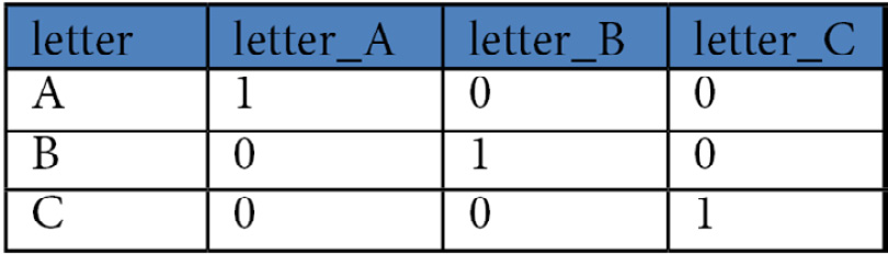
Figure 4.1 – The one-hot encoding of a categorical feature
A number of features from the NLS data are appropriate for one-hot encoding. In the following code blocks, we encode some of those features:
- Let's start by importing the OneHotEncoder module from feature_engine and loading the data. Additionally, we import the OrdinalEncoder module from scikit-learn since we will use it later:
import pandas as pd
from feature_engine.encoding import OneHotEncoder
from sklearn.preprocessing import OrdinalEncoder
from sklearn.model_selection import train_test_split
nls97 = pd.read_csv("data/nls97b.csv")
nls97.set_index("personid", inplace=True)
- Next, we create training and testing DataFrames for the NLS data:
feature_cols =['gender','maritalstatus','colenroct99']
nls97demo = nls97[['wageincome'] + feature_cols].dropna()
X_demo_train, X_demo_test, y_demo_train, y_demo_test=
train_test_split(nls97demo[feature_cols],
nls97demo[['wageincome']], test_size=0.3,
random_state=0)
- One option we have for the encoding is the pandas get_dummies method. We can use it to indicate that we want to convert the gender and maritalstatus features. get_dummies gives us a dummy variable for each value of gender and maritalstatus. For example, gender has the values of Female and Male. get_dummies creates a feature, gender_Female, which is 1 when gender is Female and 0 when gender is Male. When gender is Male, gender_Male is 1 and gender_Female is 0. This is a tried-and-true method of doing this type of encoding and has served statisticians well for many years:
pd.get_dummies(X_demo_train,
columns=['gender','maritalstatus']).head(2).T
personid 736081 832734
colenroct99 1.Not enrolled 1.Not enrolled
gender_Female 1 0
gender_Male 0 1
maritalstatus_Divorced 0 0
maritalstatus_Married 1 0
maritalstatus_Never-married 0 1
maritalstatus_Separated 0 0
maritalstatus_Widowed 0 0
We are not saving the DataFrame created by get_dummies because, later in this section, we will be using a different technique to do the encoding.
Typically, we create k-1 dummy variables for k unique values for a feature. So, if gender has two values in our data, we only need to create one dummy variable. If we know the value for gender_Female, we also know the value of gender_Male; therefore, the latter variable is redundant. Similarly, we know the value of maritalstatus_Divorced if we know the values of the other maritalstatus dummies. Creating a redundancy in this way is inelegantly referred to as the dummy variable trap. To avoid this problem, we drop one dummy from each group.
Note
For some machine learning algorithms, such as linear regression, dropping one dummy variable is actually required. In estimating the parameters of a linear model, the matrix is inverted. If our model has an intercept, and all dummy variables are included, the matrix cannot be inverted.
- We can set the get_dummies drop_first parameter to True to drop the first dummy from each group:
pd.get_dummies(X_demo_train,
columns=['gender','maritalstatus'],
drop_first=True).head(2).T
personid 736081 832734
colenroct99 1. Not enrolled 1. Not enrolled
gender_Male 0 1
maritalstatus_Married 1 0
maritalstatus_Never-married 0 1
maritalstatus_Separated 0 0
maritalstatus_Widowed 0 0
An alternative to get_dummies is the one-hot encoder in either sklearn or feature_engine. These one-hot encoders have the advantage that they can be easily brought into a machine learning pipeline, and they can persist information gathered from the training dataset to the testing dataset.
- Let's use the OneHotEncoder module from feature_engine to do the encoding. We set drop_last to True to drop one of the dummies from each group. We fit the encoding to the training data and then transform both the training and testing data:
ohe = OneHotEncoder(drop_last=True,
variables=['gender','maritalstatus'])
ohe.fit(X_demo_train)
X_demo_train_ohe = ohe.transform(X_demo_train)
X_demo_test_ohe = ohe.transform(X_demo_test)
X_demo_train_ohe.filter(regex='gen|mar', axis="columns").head(2).T
personid 736081 832734
gender_Female 1 0
maritalstatus_Married 1 0
maritalstatus_Never-married 0 1
maritalstatus_Divorced 0 0
maritalstatus_Separated 0 0
This demonstrates that one-hot encoding is a fairly straightforward way to prepare nominal data for a machine learning algorithm. But what if our categorical features are ordinal, rather than nominal? In that case, we need to use ordinal encoding.
Ordinal encoding
Categorical features can be either nominal or ordinal, as discussed in Chapter 1, Examining the Distribution of Features and Targets. Gender and marital status are nominal. Their values do not imply order. For example, "never married" is not a higher value than "divorced."
However, when a categorical feature is ordinal, we want the encoding to capture the ranking of the values. For example, if we have a feature that has the values of low, medium, and high, one-hot encoding would lose this ordering. Instead, a transformed feature with the values of 1, 2, and 3 for low, medium, and high, respectively, would be better. We can accomplish this with ordinal encoding.
The college enrollment feature on the NLS dataset can be considered an ordinal feature. The values range from 1. Not enrolled to 3. 4-year college. We should use ordinal encoding to prepare it for modeling. We will do that next:
- We can use the OrdinalEncoder module of sklearn to encode the college enrollment for 1999 feature. First, let's take a look at the values of colenroct99 prior to encoding. The values are strings, but there is an implied order:
X_demo_train.colenroct99.unique()
array(['1. Not enrolled', '2. 2-year college ',
'3. 4-year college'], dtype=object)
X_demo_train.head()
gender maritalstatus colenroct99
personid
736081 Female Married 1. Not enrolled
832734 Male Never-married 1. Not enrolled
453537 Male Married 1. Not enrolled
322059 Female Divorced 1. Not enrolled
324323 Female Married 2. 2-year college
- We can tell the OrdinalEncoder module to rank the values in the same order by passing the preceding array into the categories parameter. Then, we can use fit_transform to transform the college enrollment field, colenroct99. (The fit_transform method of the sklearn OrdinalEncoder module returns a NumPy array, so we need to use the pandas DataFrame method to create a DataFrame.) Finally, we join the encoded features with the other features from the training data:
oe = OrdinalEncoder(categories=
[X_demo_train.colenroct99.unique()])
colenr_enc =
pd.DataFrame(oe.fit_transform(X_demo_train[['colenroct99']]),
columns=['colenroct99'], index=X_demo_train.index)
X_demo_train_enc =
X_demo_train[['gender','maritalstatus']].
join(colenr_enc)
- Let's take a look at a few observations of the resulting DataFrame. Additionally, we should compare the counts of the original college enrollment feature to the transformed feature:
X_demo_train_enc.head()
gender maritalstatus colenroct99
personid
736081 Female Married 0
832734 Male Never-married 0
453537 Male Married 0
322059 Female Divorced 0
324323 Female Married 1
X_demo_train.colenroct99.value_counts().sort_index()
1. Not enrolled 3050
2. 2-year college 142
3. 4-year college 350
Name: colenroct99, dtype: int64
X_demo_train_enc.colenroct99.value_counts().sort_index()
0 3050
1 142
2 350
Name: colenroct99, dtype: int64
The ordinal encoding replaces the initial values for colenroct99 with numbers from 0 to 2. It is now in a form that is consumable by many machine learning models, and we have retained the meaningful ranking information.
Note
Ordinal encoding is appropriate for non-linear models such as decision trees. It might not make sense in a linear regression model because that would assume that the distance between values was equally meaningful across the whole distribution. In this example, that would assume that the increase from 0 to 1 (that is, from no enrollment to 2-year enrollment) is the same thing as the increase from 1 to 2 (that is, from 2-year enrollment to 4-year enrollment).
One-hot encoding and ordinal encoding are relatively straightforward approaches to engineering categorical features. It can be more complicated to deal with categorical features when there are many more unique values. In the next section, we will go over a couple of techniques for handling those features.
Encoding categorical features with medium or high cardinality
When we are working with a categorical feature that has many unique values, say 10 or more, it can be impractical to create a dummy variable for each value. When there is high cardinality, that is, a very large number of unique values, there might be too few observations with certain values to provide much information for our models. At the extreme, with an ID variable, there is just one observation for each value.
There are a couple of ways in which to handle medium or high cardinality. One way is to create dummies for the top k categories and group the remaining values into an other category. Another way is to use feature hashing, also known as the hashing trick. In this section, we will explore both strategies. We will be using the COVID-19 dataset for this example:
- Let's create training and testing DataFrames from COVID-19 data, and import the feature_engine and category_encoders libraries:
import pandas as pd
from feature_engine.encoding import OneHotEncoder
from category_encoders.hashing import HashingEncoder
from sklearn.model_selection import train_test_split
covidtotals = pd.read_csv("data/covidtotals.csv")
feature_cols = ['location','population',
'aged_65_older','diabetes_prevalence','region']
covidtotals = covidtotals[['total_cases'] + feature_cols].dropna()
X_train, X_test, y_train, y_test =
train_test_split(covidtotals[feature_cols],
covidtotals[['total_cases']], test_size=0.3,
random_state=0)
The feature region has 16 unique values, the first 6 of which have counts of 10 or more:
X_train.region.value_counts()
Eastern Europe 16
East Asia 12
Western Europe 12
West Africa 11
West Asia 10
East Africa 10
South America 7
South Asia 7
Central Africa 7
Southern Africa 7
Oceania / Aus 6
Caribbean 6
Central Asia 5
North Africa 4
North America 3
Central America 3
Name: region, dtype: int64
- We can use the OneHotEncoder module from feature_engine again to encode the region feature. This time, we use the top_categories parameter to indicate that we only want to create dummies for the top six category values. Any values that do not fall into the top six will have a 0 for all of the dummies:
ohe = OneHotEncoder(top_categories=6, variables=['region'])
covidtotals_ohe = ohe.fit_transform(covidtotals)
covidtotals_ohe.filter(regex='location|region',
axis="columns").sample(5, random_state=99).T
97 173 92 187 104
Location Israel Senegal Indonesia Sri Lanka Kenya
region_Eastern Europe 0 0 0 0 0
region_Western Europe 0 0 0 0 0
region_West Africa 0 1 0 0 0
region_East Asia 0 0 1 0 0
region_West Asia 1 0 0 0 0
region_East Africa 0 0 0 0 1
An alternative approach to one-hot encoding, when a categorical feature has many unique values, is to use feature hashing.
Feature hashing
Feature hashing maps a large number of unique feature values to a smaller number of dummy variables. We can specify the number of dummy variables to create. However, collisions are possible; that is, some feature values might map to the same dummy variable combination. The number of collisions increases as we decrease the number of requested dummy variables.
We can use HashingEncoder from category_encoders to do feature hashing. We use n_components to indicate that we want six dummy variables (we copy the region feature before we do the transform so that we can compare the original values to the new dummies):
X_train['region2'] = X_train.region
he = HashingEncoder(cols=['region'], n_components=6)
X_train_enc = he.fit_transform(X_train)
X_train_enc.
groupby(['col_0','col_1','col_2','col_3','col_4',
'col_5','region2']).
size().reset_index().rename(columns={0:'count'})col_0 col_1 col_2 col_3 col_4 col_5 region2 count
0 0 0 0 0 0 1 Caribbean 6
1 0 0 0 0 0 1 Central Africa 7
2 0 0 0 0 0 1 East Africa 10
3 0 0 0 0 0 1 North Africa 4
4 0 0 0 0 1 0 Central America 3
5 0 0 0 0 1 0 Eastern Europe 16
6 0 0 0 0 1 0 North America 3
7 0 0 0 0 1 0 Oceania / Aus 6
8 0 0 0 0 1 0 Southern Africa 7
9 0 0 0 0 1 0 West Asia 10
10 0 0 0 0 1 0 Western Europe 12
11 0 0 0 1 0 0 Central Asia 5
12 0 0 0 1 0 0 East Asia 12
13 0 0 0 1 0 0 South Asia 7
14 0 0 1 0 0 0 West Africa 11
15 1 0 0 0 0 0 South America 7
Unfortunately, this gives us a large number of collisions. For example, Caribbean, Central Africa, East Africa, and North Africa all get the same dummy variable values. In this case at least, using one-hot encoding and specifying the number of categories, as we did in the last section, was a better solution.
In the previous two sections, we covered common encoding strategies: one-hot encoding, ordinal encoding, and feature hashing. Almost all of our categorical features will require some kind of encoding before we can use them in a model. However, sometimes, we need to alter our features in other ways, including with transformations, binning, and scaling. In the next three sections, we will consider the reasons why we might need to alter our features in these ways and explore tools for doing that.
Using mathematical transformations
Sometimes, we want to use features that do not have a Gaussian distribution with a machine learning algorithm that assumes our features are distributed in that way. When that happens, we either need to change our minds about which algorithm to use (for example, we could choose KNN rather than linear regression) or transform our features so that they approximate a Gaussian distribution. In this section, we will go over a couple of strategies for doing the latter:
- We start by importing the transformation module from feature_engine, train_test_split from sklearn, and stats from scipy. Additionally, we create training and testing DataFrames with the COVID-19 data:
import pandas as pd
from feature_engine import transformation as vt
from sklearn.model_selection import train_test_split
import matplotlib.pyplot as plt
from scipy import stats
covidtotals = pd.read_csv("data/covidtotals.csv")
feature_cols = ['location','population',
'aged_65_older','diabetes_prevalence','region']
covidtotals = covidtotals[['total_cases'] + feature_cols].dropna()
X_train, X_test, y_train, y_test =
train_test_split(covidtotals[feature_cols],
covidtotals[['total_cases']], test_size=0.3,
random_state=0)
- Let's take a look at how the total number of cases by country is distributed. We should also calculate the skew:
y_train.total_cases.skew()
6.313169268923333
plt.hist(y_train.total_cases)
plt.title("Total COVID Cases (in millions)")
plt.xlabel('Cases')
plt.ylabel("Number of Countries")
plt.show()
This produces the following histogram:

Figure 4.2 – A histogram of the total number of COVID cases
This illustrates the very high skew for the total number of cases. In fact, it looks log-normal, which is not surprising given the large number of very low values and several very high values.
Note
For more information about the measures of skew and kurtosis, please refer to Chapter 1, Examining the Distribution of Features and Targets.
- Let's try a log transformation. All we need to do to get feature_engine to do the transformation is call LogTranformer and pass the feature or features that we would like to transform:
tf = vt.LogTransformer(variables = ['total_cases'])
y_train_tf = tf.fit_transform(y_train)
y_train_tf.total_cases.skew()
-1.3872728024141519
plt.hist(y_train_tf.total_cases)
plt.title("Total COVID Cases (log transformation)")
plt.xlabel('Cases')
plt.ylabel("Number of Countries")
plt.show()
This produces the following histogram:

Figure 4.3 – A histogram of the total number of COVID cases with log transformation
Effectively, log transformations increase variability at the lower end of the distribution and decrease variability at the upper end. This produces a more symmetrical distribution. This is because the slope of the logarithmic function is steeper for smaller values than for larger ones.
- This is definitely a big improvement, but there is now some negative skew. Perhaps a Box-Cox transformation will yield better results. Let's try that:
tf = vt.BoxCoxTransformer(variables = ['total_cases'])
y_train_tf = tf.fit_transform(y_train)
y_train_tf.total_cases.skew()
0.07333475786753735
plt.hist(y_train_tf.total_cases)
plt.title("Total COVID Cases (Box-Cox transformation)")
plt.xlabel('Cases')
plt.ylabel("Number of Countries")
plt.show()
This produces the following plot:
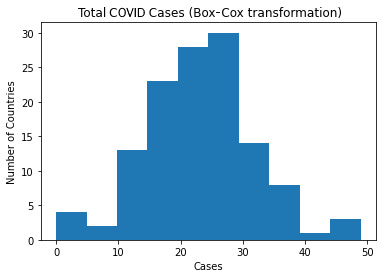
Figure 4.4 – A histogram of the total number of COVID cases with a Box-Cox transformation
Box-Cox transformations identify a value for lambda between -5 and 5 that generates a distribution that is closest to normal. It uses the following equation for the transformation:
![]()
or
![]()
Here, ![]() is our transformed feature. Just for fun, let's see the value of the lambda that was used to transform total_cases:
is our transformed feature. Just for fun, let's see the value of the lambda that was used to transform total_cases:
stats.boxcox(y_train.total_cases)[1]
0.10435377585681517
The lambda for the Box-Cox transformation is 0.104. For comparison, the lambda for a feature with a Gaussian distribution would be 1.000, meaning that no transformation would be necessary.
Now that our transformed total cases feature looks good, we can build a model with it as the target. Additionally, we can set up our pipeline to restore values to their original scaling when we make predictions. feature_engine has a number of other transformations that are implemented similarly to the log and Box-Cox transformations.
Feature binning
Sometimes, we will want to convert a continuous feature into a categorical feature. The process of creating k equally spaced intervals from the minimum to the maximum value of a distribution is called binning or, the somewhat less-friendly term, discretization. Binning can address several important issues with a feature: skew, excessive kurtosis, and the presence of outliers.
Equal-width and equal-frequency binning
Binning might be a good choice with the COVID case data. Let's try that (this might also be useful with other variables in the dataset, including total deaths and population, but we will only work with total cases for now. total_cases is the target variable in the following code, so it is a column – the only column – on the y_train DataFrame):
- First, we need to import EqualFrequencyDiscretiser and EqualWidthDiscretiser from feature_engine. Additionally, we need to create training and testing DataFrames from the COVID data:
import pandas as pd
from feature_engine.discretisation import EqualFrequencyDiscretiser as efd
from feature_engine.discretisation import EqualWidthDiscretiser as ewd
from sklearn.preprocessing import KBinsDiscretizer
from sklearn.model_selection import train_test_split
covidtotals = pd.read_csv("data/covidtotals.csv")
feature_cols = ['location','population',
'aged_65_older','diabetes_prevalence','region']
covidtotals = covidtotals[['total_cases'] + feature_cols].dropna()
X_train, X_test, y_train, y_test =
train_test_split(covidtotals[feature_cols],
covidtotals[['total_cases']], test_size=0.3, random_state=0)
- We can use the pandas qcut method, and its q parameter, to create 10 bins of relatively equal frequency:
y_train['total_cases_group'] = pd.qcut(y_train.total_cases, q=10, labels=[0,1,2,3,4,5,6,7,8,9])
y_train.total_cases_group.value_counts().sort_index()
0 13
1 13
2 12
3 13
4 12
5 13
6 12
7 13
8 12
9 13
Name: total_cases_group, dtype: int64
- We can accomplish the same thing with EqualFrequencyDiscretiser. First, we define a function to run the transformation. The function takes a feature_engine transformation and the training and testing DataFrames. It returns the transformed DataFrames (it is not necessary to define a function, but it makes sense here since we will repeat these steps later):
def runtransform(bt, dftrain, dftest):
bt.fit(dftrain)
train_bins = bt.transform(dftrain)
test_bins = bt.transform(dftest)
return train_bins, test_bins
- Next, we create an EqualFrequencyDiscretiser transformer and call the runtransform function that we just created:
y_train.drop(['total_cases_group'], axis=1, inplace=True)
bintransformer = efd(q=10, variables=['total_cases'])
y_train_bins, y_test_bins = runtransform(bintransformer, y_train, y_test)
y_train_bins.total_cases.value_counts().sort_index()
0 13
1 13
2 12
3 13
4 12
5 13
6 12
7 13
8 12
9 13
Name: total_cases, dtype: int64
This gives us the same results as qcut, but it has the advantage of being easier to bring into a machine learning pipeline since we are using feature_engine to produce it. The equal-frequency binning addresses both the skew and outlier problems.
Note
We will explore machine learning pipelines in detail in this book, starting with Chapter 6, Preparing for Model Evaluation. Here, the key point is that feature engine transformers can be a part of a pipeline that includes other sklearn-compatible transformers, even ones we construct ourselves.
- EqualWidthDiscretiser works similarly:
bintransformer = ewd(bins=10, variables=['total_cases'])
y_train_bins, y_test_bins = runtransform(bintransformer, y_train, y_test)
y_train_bins.total_cases.value_counts().sort_index()
0 119
1 4
5 1
9 2
Name: total_cases, dtype: int64
This is a far less successful transformation. Almost all of the values are at the bottom of the distribution in the data prior to the binning, so it is not surprising that equal-width binning would have the same problem. It results in only 4 bins, even though we requested 10.
- Let's examine the range of each bin. Here, we can see that the equal-width binner is not even able to construct equal-width bins because of the small number of observations at the top of the distribution:
pd.options.display.float_format = '{:,.0f}'.format
y_train_bins = y_train_bins.
rename(columns={'total_cases':'total_cases_group'}).
join(y_train)
y_train_bins.groupby("total_cases_group")["total_cases"].agg(['min','max'])
min max
total_cases_group
0 1 3,304,135
1 3,740,567 5,856,682
5 18,909,037 18,909,037
9 30,709,557 33,770,444
Although in this case, equal-width binning was a bad choice, there are many times when it makes sense. It can be useful when data is more uniformly distributed or when the equal widths make sense substantively.
K-means binning
Another option is to use k-means clustering to determine the bins. The k-means algorithm randomly selects k data points as centers of clusters and then assigns the other data points to the closest cluster. The mean of each cluster is computed, and the data points are reassigned to the nearest new cluster. This process is repeated until the optimal centers are found.
When k-means is used for binning, all data points in the same cluster will have the same ordinal value:
- We can use scikit-learn's KBinsDiscretizer to create bins with the COVID cases data:
kbins = KBinsDiscretizer(n_bins=10, encode='ordinal', strategy='kmeans')
y_train_bins =
pd.DataFrame(kbins.fit_transform(y_train),
columns=['total_cases'])
y_train_bins.total_cases.value_counts().sort_index()
0 49
1 24
2 23
3 11
4 6
5 6
6 4
7 1
8 1
9 1
Name: total_cases, dtype: int64
- Let's compare the skew and kurtosis of the original total cases variable to that of the binned variable. Recall that we would expect a skew of 0 and a kurtosis near 3 for a variable with a Gaussian distribution. The distribution of the binned variable is much closer to Gaussian:
y_train.total_cases.agg(['skew','kurtosis'])
skew 6.313
kurtosis 41.553
Name: total_cases, dtype: float64
y_train_bins.total_cases.agg(['skew','kurtosis'])
skew 1.439
kurtosis 1.923
Name: total_cases, dtype: float64
Binning can help us to address skew, kurtosis, and outliers in our data. However, it does mask much of the variation in the feature and reduces its explanatory potential. Often, some form of scaling, such as min-max or z-score, is a better option. Let's examine feature scaling next.
Feature scaling
Often, the features we want to use in our model are on very different scales. Put simply, the distance between the minimum and maximum values, or the range, varies substantially across possible features. For example, in the COVID-19 data, the total cases feature goes from 1 to almost 34 million, while aged 65 or older goes from 9 to 27 (the number represents the percentage of the population).
Having features on very different scales impacts many machine learning algorithms. For example, KNN models often use Euclidean distance, and features with greater ranges will have a greater influence on the model. Scaling can address this problem.
In this section, we will go over two popular approaches to scaling: min-max scaling and standard (or z-score) scaling. Min-max scaling replaces each value with its location in the range. More precisely, the following happens:
![]() =
= 
Here, ![]() is the min-max score,
is the min-max score, ![]() is the value for the
is the value for the ![]() observation of the
observation of the ![]() feature, and
feature, and ![]() and
and ![]() are the minimum and maximum values of the
are the minimum and maximum values of the ![]() feature.
feature.
Standard scaling normalizes the feature values around a mean of 0. Those who studied undergraduate statistics will recognize it as the z-score. Specifically, it is as follows:

Here, ![]() is the value for the
is the value for the ![]() observation of the
observation of the ![]() feature,
feature, ![]() is the mean for feature
is the mean for feature ![]() , and
, and ![]() is the standard deviation for that feature.
is the standard deviation for that feature.
We can use scikit-learn's preprocessing module to get the min-max and standard scalers:
- We start by importing the preprocessing module and creating training and testing DataFrames from the COVID-19 data:
import pandas as pd
from sklearn.model_selection import train_test_split
from sklearn.preprocessing import MinMaxScaler, StandardScaler, RobustScaler
covidtotals = pd.read_csv("data/covidtotals.csv")
feature_cols = ['population','total_deaths',
'aged_65_older','diabetes_prevalence']
covidtotals = covidtotals[['total_cases'] + feature_cols].dropna()
X_train, X_test, y_train, y_test =
train_test_split(covidtotals[feature_cols],
covidtotals[['total_cases']], test_size=0.3, random_state=0)
- Now, we can run the min-max scaler. The fit_transform method for sklearn will return a numpy array. We convert it into a pandas DataFrame using the columns and index from the training DataFrame. Notice how all features now have values between 0 and 1:
scaler = MinMaxScaler()
X_train_mms = pd.DataFrame(scaler.fit_transform(X_train),
columns=X_train.columns, index=X_train.index)
X_train_mms.describe()
population total_deaths aged_65_older diabetes_prevalence
count 123.00 123.00 123.00 123.00
mean 0.04 0.04 0.30 0.41
std 0.13 0.14 0.24 0.23
min 0.00 0.00 0.00 0.00
25% 0.00 0.00 0.10 0.26
50% 0.01 0.00 0.22 0.37
75% 0.02 0.02 0.51 0.54
max 1.00 1.00 1.00 1.00
- We run the standard scaler in the same manner:
scaler = StandardScaler()
X_train_ss = pd.DataFrame(scaler.fit_transform(X_train),
columns=X_train.columns, index=X_train.index)
X_train_ss.describe()
population total_deaths aged_65_older diabetes_prevalence
count 123.00 123.00 123.00 123.00
mean -0.00 -0.00 -0.00 -0.00
std 1.00 1.00 1.00 1.00
min -0.29 -0.32 -1.24 -1.84
25% -0.27 -0.31 -0.84 -0.69
50% -0.24 -0.29 -0.34 -0.18
75% -0.11 -0.18 0.87 0.59
max 7.58 6.75 2.93 2.63
If we have outliers in our data, robust scaling might be a good option. Robust scaling subtracts the median from each value of a variable and divides that value by the interquartile range. So, each value is as follows:

Here, ![]() is the value of the
is the value of the ![]() feature, and
feature, and ![]() ,
, ![]() ,and
,and ![]() are the median, third, and first quantiles of the
are the median, third, and first quantiles of the ![]() feature. Robust scaling is less sensitive to extreme values since it does not use the mean or variance.
feature. Robust scaling is less sensitive to extreme values since it does not use the mean or variance.
- We can use scikit-learn's RobustScaler module to do robust scaling:
scaler = RobustScaler()
X_train_rs = pd.DataFrame(
scaler.fit_transform(X_train),
columns=X_train.columns, index=X_train.index)
X_train_rs.describe()
population total_deaths aged_65_older diabetes_prevalence
count 123.00 123.00 123.00 123.00
mean 1.47 2.22 0.20 0.14
std 6.24 7.65 0.59 0.79
min -0.35 -0.19 -0.53 -1.30
25% -0.24 -0.15 -0.30 -0.40
50% 0.00 0.00 0.00 0.00
75% 0.76 0.85 0.70 0.60
max 48.59 53.64 1.91 2.20
We use feature scaling with most machine learning algorithms. Although it is not often required, it yields noticeably better results. Min-max scaling and standard scaling are popular scaling techniques, but there are times when robust scaling might be the better option.
Summary
In this chapter, we covered a wide range of feature engineering techniques. We used tools to drop redundant or highly correlated features. We explored the most common kinds of encoding – one-hot encoding, ordinal encoding, and hashing encoding. Following this, we used transformations to improve the distribution of our features. Finally, we used common binning and scaling approaches to address skew, kurtosis, and outliers, and to adjust for features with widely different ranges.
Some of the techniques we discussed in this chapter are required for most machine learning models. We almost always need to encode our features for algorithms in order to understand them correctly. For example, most algorithms cannot make sense of female or male values or know not to treat ZIP codes as ordinal. Although not typically necessary, scaling is often a very good idea when we have features with vastly different ranges. When we are using algorithms that assume a Gaussian distribution of our features, some form of transformation might be required for our features to be consistent with that assumption.
We now have a good sense of how our features are distributed, have imputed missing values, and have done some feature engineering where necessary. We are now prepared to begin perhaps the most interesting and meaningful part of the model building process – feature selection.
In the next chapter, we will examine key feature selection tasks, building on the feature cleaning, exploration, and engineering work that we have done so far.