10

Self-Supervised Learning

Imagine that you are in the middle of the ocean, and you are thirsty. There is water all around you, but you cannot drink any of it. But what if you had the resources to boil the salt out of the water and thereby make it drinkable? Of course, the energy costs associated with the process can be quite high, so you will likely use the process in moderation. However, if your energy costs effectively became free, for example, if you were harnessing the power of the sun, the process might be more attractive for you to do on a larger scale.

In our somewhat simplistic situation described above, the first scenario is roughly analogous to supervised learning, and the second to the class of unsupervised / semi-supervised learning techniques we will cover in this chapter. The biggest problem with supervised learning techniques is the time and expense associated with the collection of labeled training data. As a result, labeled datasets are often relatively small.

Deep learning trades off computation against manual feature engineering, and while this can be very effective, deep learning models typically need more data to train than traditional (non-deep learning) models. Deep learning models tend to be more complex and have more learnable parameters, which results in them performing better at various tasks. However, more complex models also require more data to train. Because the creation of training data is expensive, this effectively limits us from scaling up Deep learning models using supervised learning.

Unfortunately, completely unsupervised learning techniques that do not need labeled data have had limited success so far. Self-supervised techniques that leverage the structure of data in the wild to create labeled data to feed supervised learning models offer a middle ground. In this chapter, we will learn about various self-supervised techniques and some of their applications in the areas of natural language processing, computer vision, and audio signal processing.

The chapter covers the following topics:

• Previous work
• Self-supervised learning
• Self-prediction
• Contrastive learning
• Pretext tasks

Self-supervised learning is the process of imaginatively reusing labels that already exist implicitly in your data. In this chapter, we will learn about some common strategies for self-supervised learning and examples of their use to solve real-life problems. Let’s begin.

Previous work

Self-supervised learning is not a new concept. However, the term became popular with the advent of transformer-based models such as BERT and GPT-2, which were trained in a semi-supervised manner on large quantities of unlabeled text. In the past, self-supervised learning was often labeled as unsupervised learning. However, there were many earlier models that attempted to leverage regularities in the input data to produce results comparable to that using supervised learning. You have encountered some of them in previous chapters already, but we will briefly cover them again in this section.

The Restricted Boltzmann Machine (RBM) is a generative neural model that can learn a probability distribution over its inputs. It was invented in 1986 and subsequently improved in the mid-2000s. It can be trained in either supervised or unsupervised mode and can be applied to many downstream tasks, such as dimensionality reduction, classification, etc.

Autoencoders (AEs) are unsupervised learning models that attempt to learn an efficient latent representation of input data by learning to reconstruct its input. The latent representation can be used to encode the input for downstream tasks. There are several variants of the model. Sparse, denoising, and contrastive AEs are effective in learning representations for downstream classification tasks, whereas variational AEs are more useful as generative models.

The Word2Vec model is another great example of what we would now call self-supervised learning. The CBOW and skip-gram models used to build the latent representation of words in a corpus, attempt to learn mappings of neighbors to words and words to neighbors respectively. However, the latent representation can now be used as word embeddings for a variety of downstream tasks. Similarly, the GloVe model is also a self-supervised model, which uses word co-occurrences and matrix factorization to generate word embeddings useful for downstream tasks.

Autoregressive (AR) models predict future behavior based on past behavior. We cover them in this chapter in the Self-prediction section. However, AR models have their roots in time series analysis in statistics, hidden Markov models in pre-neural natural language processing, Recurrent Neural Networks (RNNs) in neural (but pre-transformer) NLP.

Contrastive Learning (CL) models try to learn representations whereby similar pairs of items cluster together and dissimilar pairs are pushed far apart.

CL models are also covered in this chapter in the Contrastive learning section. However, Self Organizing Maps (SOMs) and Siamese networks use very similar ideas and may have been a precursor of current CL models.

Self-supervised learning

In self-supervised learning, the network is trained using supervised learning, but the labels are obtained in an automated manner by leveraging some property of the data and without human labeling effort. Usually, this automation is achieved by leveraging how parts of the data sample interact with each other and learning to predict that. In other words, the data itself provides the supervision for the learning process.

One class of techniques involves leveraging co-occurrences within parts of the same data sample or co-occurrences between the same data sample at different points in time. These techniques are discussed in more detail in the Self-prediction section.

Another class of techniques involves leveraging co-occurring modality for a given data sample, for example, between a piece of text and its associated audio stream, or an image and its caption. Examples of this technique are discussed in the sections on joint learning.

Yet another class of self-supervised learning techniques involves exploiting relationships between pairs of data samples. These pairs are selected from the dataset based on some domain-level heuristic. Examples of these techniques are covered in the Contrastive learning section.

These techniques can either be used to train a model to learn to solve a business task (such as sentiment analysis, classification, etc.) directly or to learn a latent (embedding) representation of the data that can then be used to generate features to learn to solve a downstream business task. The latter class of tasks that are used to indirectly learn the latent representation of the data are called pretext tasks. The Pretext tasks section will cover this subject, with examples, in more detail.

The advantages of self-supervised learning are twofold. First, as noted already, supervised learning involves the manual labeling of data, which is very expensive to create, and therefore it is difficult to get high-quality labeled data. Second, self-supervised tasks may not address a business task directly but can be used to learn a good representation of the data, which can then be applied to transfer this information to actual business tasks downstream.

Self-prediction

The idea behind self-prediction is to predict one part of a data sample given another part. For the purposes of prediction, we pretend that the part to be predicted is hidden or missing and learn to predict it. Obviously, both parts are known, and the part to be predicted serves as the data label. The model is trained in a supervised manner, using the non-hidden part as the input and the hidden part as the label, learning to predict the hidden part accurately. Essentially, it is to pretend that there is a part of the input that you don’t know and predict that.

The idea can also be extended to reversing the pipeline, for example, deliberately adding noise to an image and using the original image as the label and the corrupted image as the input.

Autoregressive generation

Autoregressive (AR) models attempt to predict a future event, behavior, or property based on past events, behavior, or properties. Any data that comes with some innate sequential order can be modeled using AR generation. Unlike latent variable models such as VAEs or GANs, AR models make no assumptions of independence.

PixelRNN

The PixelRNN [1] AR model uses two-dimensional Recurrent Neural Networks (RNNs) to model images on a large scale. The idea is to learn to generate a pixel by conditioning on all pixels to the left and above it. A convolution operation is used to compute all the states along each dimension at once. The LSTM layers used in PixelRNN are one of two types – the Row LSTM and the Diagonal BiLSTM. In the row LSTM, the convolution is applied along each row, and in the Diagonal BiLSTM, the convolutions are applied along the diagonals of the image:

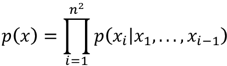
Figure 10.1: PixelRNN tries to predict a pixel by conditioning on all pixels to the left and above it. From the paper Pixel Recurrent Neural Networks [1]

Image GPT (IPT)

Image GPT (IPT) [14] is similar to PixelRNN except it works on patches, and each patch is treated as a word. The Image GPT is based on the Transformer model and is trained on images from the ImageNet dataset. The images are corrupted in multiple different ways (super-resolution, bicubic interpolation, adding noise, etc.) and pretrained to predict the original image. The core of the IPT model consisted of a transformer encoder decoder pair but had multiple heads and tails to extract features from the corrupted input image and format the decoder output into the output image respectively. The multiple heads and tails were specialized for each of the different tasks IPT is trained to do (denoising, de-raining, x2 and x4 super-resolution, etc.):

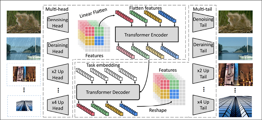
Figure 10.2: Architecture of the Image GPT (IPT) AR model. From the paper Pre-trained Image Processing Transformer [14]

GPT-3

The GPT-3, or Generative Pre-trained Transformer [9] model from OpenAI is an AR language model that can generate human-like text. It generates sequences of words, code, and other data, starting from a human-provided prompt. The first version of GPT used 110 million learning parameters, GPT-2 used 1.5 billion, and GPT-3 used 175 billion parameters. The model is trained on unlabeled text such as Wikipedia that is readily available on the internet, initially in English but later in other languages as well. The GPT-3 model has a wide variety of use cases, including summarization, translation, grammar correction, question answering, chatbots, and email composition.

The popularity of GPT-3 has given rise to a new profession called prompt engineering [39], which is basically to create the most effective prompts to start GPT-3 on various tasks. A partial list of possible applications for GPT-3 can be found on the OpenAI GPT-3 examples page (https://beta.openai.com/examples/).

XLNet

XLNet [38] is similar to GPT-3 in that it is a generalized AR model. However, it leverages both AR language modeling and AutoEncoding while avoiding their limitations. Instead of using only tokens from the left or right context to predict the next token, it uses all possible permutations of the tokens from the left and right contexts, thus using tokens from both the left and right contexts for prediction. Secondly, unlike AE approaches such as BERT, it does not depend on input corruption (as in masked language modeling) since it is a generalized AR language model. Empirically, under comparable experimental settings, XLNet consistently outperforms BERT on a wide spectrum of tasks.

WaveNet

WaveNet [3] is an AR generative model based on PixelCNN’s architecture but operates on the raw audio waveform. As with PixelCNN, an audio sample at a particular point in time is conditioned on the samples at all previous timesteps. The conditional probability distribution is modeled as a stack of convolutional layers. The main ingredient of the WaveNet is causal convolutions. The predictions emitted by the model at a time step cannot depend on any future timesteps. When applied to text to speech, WaveNet yields state-of-the-art performance, with human listeners rating it as significantly more natural sounding for English and Mandarin than comparable text-to-speech models.

WaveRNN

WaveRNN [28] is an AR generative model that learns the joint probability of the data by factorizing the distribution into a product of conditional probabilities over each sample. The convolutional layers of the WaveNet architecture are replaced with a single-layer RNN. It also uses more efficient sampling techniques that, overall, reduce the number of operations to perform and result in approximately 4x speedup over WaveNet.

Masked generation

Masked generation models mask some random portion of themselves and pretend it is missing, and the models learn to predict the masked information using the unmasked information available to them. Unlike autoregressive models, in the case of masked generation models, there is no need for the masked information to be located before or after the unmasked information; it can be anywhere in the input.

BERT

BERT [16], or Bidirectional Encoder Representation from Transformers, is a transformer-based language model that was trained using text from the internet by a team from Google. It uses two objectives during the pretraining phase – Masked Language Modeling (MLM) and Next Sentence Prediction (NSP). During training, 15% of the input tokens are masked and the model learns to predict the masked token. Since the model is transformer based, it can use context from anywhere in the sentence to help with predicting the masked tokens. BERT models, once pretrained, can be fine-tuned with smaller supervised datasets for a variety of downstream tasks such as classification, sentiment analysis, textual entailment, etc. BERT is covered in more depth in Chapter 6, Transformers.

You can see BERT’s masked generation in action using a pretrained BERT model from the Hugging Face Transformers library and the code snippet shown below. Here, we ask a pretrained BERT transformer model to predict the masked token [MASK] in the sentence "The capital of France is [MASK].":

from transformers import BertTokenizer, TFBertForMaskedLM
import tensorflow as tf
tokenizer = BertTokenizer.from_pretrained("bert-base-cased")
model = TFBertForMaskedLM.from_pretrained("bert-base-cased")
inputs = tokenizer("The capital of France is [MASK].", return_tensors="tf")
logits = model(**inputs).logits
mask_token_index = tf.where(inputs.input_ids == tokenizer.mask_token_id)[0][1]
predicted_token_id = tf.math.argmax(logits[:, mask_token_index], axis=-1)
print(tokenizer.convert_ids_to_tokens(predicted_token_id)[0])

Somewhat predictably, the output of this code block is "Paris".

Stacked denoising autoencoder

A stacked denoising autoencoder (AE) [29] adds random noise to images and uses them as input to a denoising AE to predict the original image. Multiple layers of denoising AEs are each individually trained and stacked. This results in the composition of several levels of non-linearity and is key to achieving better generalization performance on difficult image recognition tasks. Higher-level representations learned in this purely unsupervised manner can be used as image features to boost the performance of downstream SVM based image classifiers. Each layer functions like a regular AE, i.e., it takes an image as input and tries to reconstruct it after it passes through a “bottleneck” layer. The bottleneck layer learns a compact feature representation of the input image. Unfortunately, AEs usually end up only learning how to compress the image without learning a semantically meaningful representation. Denoising AEs address this issue by corrupting the input and requiring the network to undo the corruption and hence learn a better semantic representation of the input image.

Context autoencoder

The context autoencoder [12] masks out a region of the image and uses it to train a convolutional neural network (the context AE) to regress the missing pixel values to predict the original image. The task of a context AE is even harder than that of a denoising AE since it has to fill in larger missing areas and cannot use information from immediately neighboring pixels. This requires a much deeper semantic understanding of the image, and the ability to generate high-level features over large spatial areas. In a sense, the context AE is a more powerful generative model since it needs to fill in the missing region while maintaining coherence with the supplied context.

For that reason, the context AE is trained to reconstruct a combination of reconstruction loss and adversarial loss. This results in sharper predictions than training on reconstruction (L2) loss alone:

Figure 10.3: Qualitative illustration of the context encoder task (from Context Encoders: Feature Learning by Inpainting [10])

Context does not have to be image features, it could also be color, as we will see in the next section.

Colorization

The paper Colorization as a Proxy Task for Visual Understanding [12] uses colorization as a way to learn image representations. Color images are converted to their grayscale equivalent, which is then used as input to predict the original color image. The model can be used to automatically colorize grayscale images, as well as learn a representation that can help in downstream tasks such as image classification and segmentation. In functional terms, the model predicts the a and b (color information) channels in their Lab encoding given their L (grayscale) channel. Experiments on the ImageNet dataset by the authors of this paper have resulted in models that produce state-of-the-art results against datasets for semantic segmentation and image classification for models that don’t use ImageNet labels, and even surpass some earlier models that have been trained on ImageNet using supervised learning.

Innate relationship prediction

Models using this technique attempt to learn visual common-sense tasks by leveraging innate relationships between parts of an input image. Weights from these learned models could be used to generate semantic representations of images for other downstream tasks.

Relative position

The paper Unsupervised Visual Representation Learning by Context Prediction [8] predicts the relative position of one patch in an image with respect to another. Effectively, this approach uses spatial context as a source of self-supervision for training visual representations. Given a large unlabeled image collection, random pairs of patches are extracted from each image as shown in Figure 10.4. Each pair is labeled depending on the orientation of the second patch with respect to the central one. A convolutional network is trained to predict the position of the second patch relative to the first. The feature representation learned is found to capture the notion of visual similarity across images. Using this representation, it has been shown to aid in visual data mining, i.e., discovering image fragments that depict the same semantic object, against the Pascal VOC 2007 dataset:

Figure 10.4: Illustration of relative position prediction. The model must predict the configuration of the second patch relative to the (central) first patch. From the paper Unsupervised Visual Representation Learning by Context Prediction [8]

Solving jigsaw puzzles

The paper Unsupervised Learning of Visual Representations by Solving Jigsaw Puzzles [26] describes an approach somewhat similar to the previous approach of predicting relative position. This method attempts to learn the visual representation of images by solving jigsaw puzzles of natural images. Patches are extracted from the input image and shuffled to form a jigsaw puzzle. The network learns to reconstruct the original image from the jigsaw puzzle, i.e., to solve the jigsaw puzzle. The network used is a Context Free Network (CFN), an n-way Siamese network. Each patch corresponds to a column in the n-way CFN. The shared layers in each column are implemented exactly as in AlexNet. The classification head predicts the original index of the patch (before shuffling). On the Pascal VOC dataset, it outperforms all previous self-supervised models in image classification and object detection tasks:

Figure 10.5: The image is split up into patches and shuffled, and the model learns to put the shuffled patches back in the correct order. From the paper Unsupervised Learning of Visual Representations [26]

Rotation

The RotNet model [34] learns an image representation by using rotation as a self-supervision signal. Input images are rotated by 0, 90, 180, and 270 degrees, and a convolutional network (RotNet) is trained to learn to predict the rotation angle as one of 4 target classes. It turns out that this apparently simple task provides a very powerful supervisory signal for semantic feature learning. RotNet features were used as input for image classification against the CIFAR-10 dataset and resulted in classification accuracy of only 1.6% less than the state-of-the-art result obtained using supervised learning. It also obtained state-of-the-art results at the time for some classification tasks against ImageNet, and some classification and object detection tasks against Pascal VOC.

Hybrid self-prediction

With hybrid self-prediction models, self-prediction is achieved using not one but multiple self-prediction strategies. For example, our first two examples, Jukebox and DALL-E, achieve self-prediction by first reducing the input data to a more manageable format using one self-supervision technique (VQ-VAE or Vector Quantized Variational AutoEncoder [35]) and then use another (AR) on the reduced image to produce the final prediction. In our third example, the predictions from the VQ-VAE component are further refined using a discriminator trained in an adversarial manner.

VQ-VAE

Since the VQ-VAE is common to all our hybrid self-prediction models, let us try to understand what it does at a high level. You have already read about autoencoders and variational autoencoders in Chapter 8, Autoencoders. Autoencoders try to learn to reconstruct their input by first encoding the input onto a smaller dimension and then decoding the output of the smaller dimension. However, autoencoders typically just end up compressing the input and do not learn a good semantic representation.

Variational Autoencoders (VAEs) can do better in this respect by enforcing a probabilistic prior, generally in the form of a standard Gaussian distribution, and by minimizing not only the reconstruction loss but also the KL divergence between the prior distribution and posterior distribution (the actual distribution in the latent space).

While the VAE learns a continuous latent distribution, the VQ-VAE learns a discrete latent distribution. This is useful because transformers are designed to take discrete data as input. VQ-VAE extends VAE by adding a discrete codebook component to the network, which is used to quantize the latent vectors output by the encoder by choosing the vector in the codebook that is closest to each latent vector by Euclidean distance. The VQ-VAE decoder is then tasked with reconstructing the input from the discretized latent vector.

Jukebox

Our first example is the Jukebox paper [32], which is a generative model for music, similar to how GPT-3 is a generative model for text and Image-GPT is a generative model for images. That is, given a musical (voice and music) prompt, Jukebox can create the music that might follow this prompt. Early attempts at generative models for audio attempted symbolic music generation in the form of a piano roll, since the problem with generating raw audio directly is the extremely large amount of information it contains and consequently, the extreme long-range dependencies that need to be modeled. The VQ-VAE addresses this problem by learning a lower-dimensional encoding of the audio with the goal of losing the least important information but retaining most of the useful information.

Jukebox uses hierarchical VQ-VAEs to discretize the input signal into different temporal resolutions, then generates a new sequence at each resolution, and finally combines the generated sequence at each level into the final prediction.

DALL-E

Our second example of hybrid prediction models is the DALL-E model [5] from OpenAI. DALL-E can also be classified as a joint learning (multimodal) model, since it attempts to learn to create images from text captions, using pairs of text and image as training input. However, we classify it here as a hybrid prediction model because, like Jukebox, it attempts to address the high dimensionality of image information (compared with the dimensionality of the associated text) using a VQ-VAE.

DALL-E receives text and images as a single stream of data. DALL-E uses a two-stage training regime. In the first stage, a VQ-VAE is trained to compress each input RGB image of size (256, 256, 3) into a grid of image tokens of size (32, 32), each element of which can assume one of 8,192 possible discrete values. This reduces the size of the image input by a factor of 192 without a corresponding loss in image quality.

In the second stage, the text is BPE-encoded and truncated to 256 tokens. Byte Pair Encoding (BPE) is a hybrid character/word encoding that can represent large corpora using a relatively small vocabulary by encoding common byte pairs. This encoding is then concatenated with the flattened sequence of 1,024 (32 x 32) image tokens. This combined sequence is used to train an autoregressive transformer to model the joint distribution over the text and image tokens. The first stage learns the visual codebook in the VQ-VAE and the second stage learns the prior of the discrete latent distribution over the text and image tokens. The trained DALL-E model can then be used to generate images given a text prompt.

Text-to-image generation is getting quite popular. A newer version of DALL-E, called DALL-E 2, was recently released by OpenAI. It has 35 billion parameters compared to DALL-E’s 12 billion. Even though they are named similarly, DALL-E is a version of GPT-3 trained to generate images from text descriptions, and DALL-E 2 is an encoder-decoder pipeline that uses CLIP to encode the text description into a CLIP embedding, and then decode the embedding back to an image using a diffusion model that you learned about in Chapter 9, Generative Models. As expected, DALL-E 2 generates more realistic and accurate images than DALL-E.

Even more recently, Google Research has released Imagen, another model in this space that competes with DALL-E 2. Like DALL-E 2, Imagen uses a T5-XXL encoder to map input text into embeddings and a diffusion model to decode the embedding into an image.

VQ-GAN

The VQ-GAN [30] uses an encoder-decoder framework where the encoder uses a VQ-VAE style encoder that learns a discrete latent representation, but the decoder is a discriminator component of a Generative Adversarial Network (GAN). Instead of the L2 loss used in the VQ-VAE, the VQ-GAN uses a combination of perceptual loss and discriminator loss, which helps in keeping good perceptual quality at increased compression rates. The use of a GAN architecture rather than a traditional VAE decoder helps with training efficiency.

Like VQ-VAE, the VQ-GAN learns a codebook of context-rich visual components, which are used to compose sequences for training the autoregressive component. The VQ-GAN has been found to outperform the VQ-VAE-2 model on images from ImageNet using the Fréchet Inception Distance (FID), which measures the distance between feature vectors of real versus fake images) metric, even though it uses approximately 10x fewer parameters:

Figure 10.6: Architecture of the VQ-GAN. From the paper: Taming Transformers for High Resolution Image Synthesis [30]

Next, we will look at another popular self-supervised technique called contrastive learning.

Contrastive learning

Contrastive Learning (CL) tries to predict the relationship between a pair of input samples. The goal of CL is to learn an embedding space where pairs of similar samples are pulled close together and dissimilar samples are pushed far apart. Inputs to train CL models are in the form of pairs of data points. CL can be used in both supervised and unsupervised settings.

When used in an unsupervised setting, it can be a very powerful self-supervised learning approach. Similar pairs are found from existing data in a self-supervised manner, and dissimilar pairs are found from pairs of similar pairs of data. The model learns to predict if a pair of data points are similar or different.

A taxonomy of CL can be derived by considering the techniques used to generate contrastive examples. Before we do that, we will take a brief detour to explore the various training objectives that are popular in CL.

Training objectives

Early CL models used data points consisting of a single positive and a single negative example to learn from. However, the trend in more recent CL models is to learn from multiple positive and negative samples in a single batch. In this section, we will cover some training objectives (also called loss functions) that are commonly used for training CL models.

Contrastive loss

Contrastive loss [35] is one of the earliest training objectives to be used for learning using CL techniques. It tries to encode data into an embedding space such that examples from the same class have similar embeddings and examples from different classes have dissimilar embeddings. Thus, given two data pairs, (x_i, y_i) and (x_j, y_j), the contrastive loss objective is described using the following formula:

The first term is activated when the pairs i and j are similar, and the second term is activated when the pair is dissimilar. The objective is designed to maximize the square of the differences in the first term and minimize the square of differences in the second term (thus maximizing the second term in the case of dissimilar pairs). The is a hyperparameter and represents a margin of the minimum allowable distance between samples of different classes.

Triplet loss

Triplet loss [11] is an enhancement of contrastive loss in that it uses three data points instead of two – the anchor point, the positive point, and the negative point. Thus, given an anchor point x, we select a positive sample and one negative sample , where x and belong to the same class and x and belong to different classes. Triplet loss learns to minimize the distance between the anchor x and positive sample and maximize the distance between x and negative sample . This is illustrated in Figure 10.7:

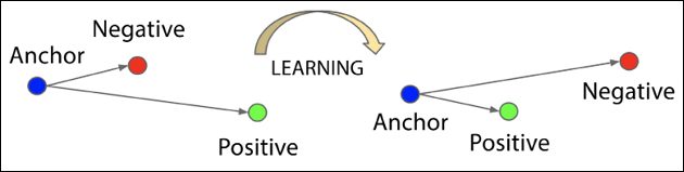
Figure 10.7: Illustration of triplet loss. Based on the paper: FaceNet: A Unified Embedding for Face Recognition and Clustering [11]

The equation for triplet loss is shown below. As with contrastive loss, the is a hyperparameter representing the minimum allowed difference between distances between similar and dissimilar pairs. Triplet loss-based models typically need challenging values for , the so-called hard negatives, to provide good representations:

N-pair loss

N-pair loss [21] generalizes triplet loss to incorporate comparison with multiple negative samples instead of just one. Thus, given an (N+1) tuple of training samples, {x, x⁺, x₁^-, x₂^-, …, x_N+1^-}, where there is one positive sample and N-1 negative ones, the N-pair loss is defined using the following equation:

Lifted structural loss

Lifted structured loss [15] is another generalization of triplet loss where it uses all pairwise edges within a training batch. This leads to better training performance. Figure 10.8 illustrates the idea behind lifted structural loss, and how it evolved from contrastive and triplet loss. Red edges connect similar pairs and blue edges connect dissimilar pairs:

Figure 10.8: Illustration of the idea of Lifted Structured Loss. Based on the paper: Deep Metric Learning via Lifted Structured Feature Embedding [15]

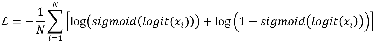
NCE loss

Noise Contrastive Estimation (NCE) loss [27] uses logistic regression to distinguish positive and negative (noise) examples. The NCE loss attempts to maximize the log odds (logits) of positive examples x and minimize the log odds of negative examples . The equation for NCE loss is shown below:

InfoNCE loss

InfoNCE loss [2] was inspired by NCE loss (described in the previous section) and uses categorical cross-entropy loss to identify the positive sample from the set of unrelated noise samples. Given some context vector c, the positive sample should be drawn from the conditional probability distribution p(x|c), while the N-1 negative examples can be drawn from the distribution p(x) independent of the context c. The InfoNCE loss optimizes the negative log probability of classifying the positive sample correctly.

The InfoNCE loss is given by the following equation, where f(x, c) estimates the density ratio p(x|c) / p(x):

Soft nearest neighbors loss

Soft nearest neighbors loss [33] further extends the idea of contrastive loss to include multiple positive samples given known labels. Given a batch of samples, 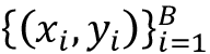where y_i is the class label of x_i, and a similarity function f that measures similarity between two inputs, the soft nearest neighbor loss is given by the equation:

The temperature is a hyperparameter and is used for tuning how concentrated the features are in the representation space. Thus, at low temperatures, the contribution of faraway points in the representation space to the soft nearest neighbors loss is also low.

Instance transformation

CL models that use instance transformation generally rely on data augmentation techniques to generate positive pairs and negative mining to generate negative pairs from pairs of positive pairs. Many such models rely on generating in-batch negative and innovative techniques for mining hard negatives.

Data augmentation techniques are used to create pairs of the original data point and its noisy version. This introduces non-essential variation into the examples without modifying semantic meaning, which the model then learns during training.

In-batch negative sampling is a technique for generating negative samples by combining information from examples within a single batch. For each positive pair (x_i, y_i) in the batch, all pairs (x_i, y_j) and (x_j, y_i) for all can be considered as negative pairs. In effect, negative pairs are created by combining elements from two random positive pairs in the same batch. This technique is practical and can be implemented efficiently on GPUs and is therefore widely used.

Some models require hard negative samples to learn how to perform their tasks well. Hard negatives are pairs that have different labels, but whose embedding features are very close to each other. You can visualize them as points that lie very close to each other in the embedding space but on opposite sides of the decision boundary. Identifying hard negatives for a given task is relatively easy for supervised learning. For unsupervised learning, one approach is to increase the batch size, which will introduce more hard negative samples. Another technique [19] is to increase the sampling probability of the candidate negative sample by its similarity with the anchor sample.

SimCLR

The SimCLR model [36] presents a simple framework for contrastive learning of visual representations. Each input image (x) is augmented in two different ways (x_i and x_j) using the same family of image augmentation strategies, resulting in 2N positive samples.

In-batch negative sampling is used, so for each positive example, we have (2N-1) negative samples. A base encoder (f) is applied to the pair of data points in each example, and a projection head (g) attempts to maximize the agreement for positive pairs and minimize it for negative pairs. For good performance, SimCLR needs to use large batch sizes so as to incorporate enough negative examples in the training regime. SimCLR achieved state-of-the-art results for self-supervised and semi-supervised models on ImageNet and matches the performance of a supervised ResNet-50. Figure 10.9 shows the architecture of the SimCLR model:

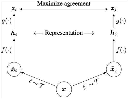
Figure 10.9: Architecture of the SimCLR model. From the paper: A Simple Framework for Contrastive Learning of Visual Representations [36]

Barlow Twins

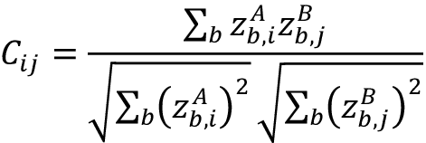
The idea behind the Barlow Twins [20] model has its roots in neuroscience, i.e., the goal of sensory processing is to re-code highly redundant sensory inputs into a factorial code, or a code with statistically independent components. In this model, an image is distorted into two versions of itself. The distorted versions are fed into the same network to extract features and learn to make the cross-correlation matrix between these two features as close to the identity matrix as possible. In line with the neuroscience idea, the goal of this model is to reduce the redundancy between the two distorted versions of the sample by reducing the redundancy between these vectors. This is reflected in its somewhat unique loss function – in the first equation, the first term represents the difference between the identity matrix and the cross-correlation matrix, and the second term represents the redundancy reduction term. The second equation defines each element of the cross-correlation matrix C:

Some notable differences between the Barlow Twins model and other models in this genre are that the Barlow Twins model doesn’t require a large number of negative samples and can thus operate on smaller batches, and that it benefits from high-dimensional embeddings. The Barlow Twins model outperforms some previous semi-supervised models trained on ImageNet and is on par with some supervised ImageNet models.

BYOL

The Bootstrap Your Own Latent (BYOL) model [17] is unique in that it does not use negative samples at all. It relies on two neural networks, the online and target networks, that interact and learn from each other. The goal of BYOL is to learn a representation that can be used for downstream tasks. The online network is parameterized by a set of weights and comprises three stages – an encoder , a projector , and a predictor The target network has the same architecture as the online network but uses a different set of weights . The target network provides the regression targets to train the online network, and its parameters are an exponential moving average of the online parameters After every training step, the following update is performed:

BYOL produces two augmented views of each image. From the first augmented view, the online network outputs a representation and a projection . Similarly, the target network outputs a representation and a projection BYOL attempts to minimize the error between the L2 normalized online and target projections and . At the end of the training, we only retain the online network (the encoder).

BYOL achieves competitive results against semi-supervised or transfer learning models on ImageNet. It is also less sensitive to changes in batch size and the type of image augmentations used compared to other models in this genre. However, later work [4] indicates that the batch normalization component in BYOL may implicitly cause a form of contrastive learning by implicitly creating negative samples as a result of data redistribution it causes.

Feature clustering

Feature clustering involves finding similar data samples by clustering them. This can be useful when data augmentation techniques are not feasible. The idea here is to use clustering algorithms to assign pseudo-labels to samples such that we can run intra-sample CL. Although similar, feature clustering differs from CL in that it relaxes the instance discrimination problem – rather than learn to distinguish between a pair of transformations on a single input image, feature clustering learns to discriminate between groups of images with similar features.

DeepCluster

The DeepCluster [24] paper is predicated on the fact that datasets for supervised learning such as ImageNet are “too small” to account for general-purpose features that go beyond image classification. For learning general-purpose features, it is necessary to train on billions of images at internet scales. However, labeling such large datasets is not feasible, so DeepCluster presents a clustering method that jointly learns the parameters of the neural network and the cluster assignments of the resulting features. DeepCluster iteratively groups these features using the K-Means clustering algorithm and uses the cluster assignments as pseudo labels to learn the parameters of the ConvNet. The end product of the training is the weights of the ConvNet. These weights have been shown to be useful general-purpose visual features and have outperformed the best published numbers on many downstream tasks regardless of the dataset.

SwAV

In the SwAV (SWapping Assignments between multiple Views) [25] model, features are learned by predicting the cluster assignment (pseudo-label) for a view from the representation of another view. SwAV uses a variant of the architecture used in CL models. The images x₁ and x₂ are transformations of the same input image x, which are sent through an encoder to produce a representation z₁ and z₂. In the case of SwAV, z₁ and z₂ are used to compute q₁ and q₂ by matching their features to a set of K prototype vectors {c₁, …, c_K}, which are then used to predict the cluster assignment for x₂ and x₁ respectively.

Unlike DeepCluster, SwAV does online clustering (clustering of data that arrives continuously in a streaming manner and is not known before the clustering process begins) and can therefore scale to potentially unlimited amounts of data. SwAV also works well with both large and small batch sizes. The SwAV paper also proposes a new multi-crop strategy to increase the number of views of an image with no computational or memory overhead. It achieves 75% top-1 accuracy on ImageNet with ResNet50 (a supervised learning method) as well as surpassing results of supervised pretraining in all the considered transfer tasks.

InterCLR

InterCLR [18] is a hybrid model that jointly learns a visual representation by leveraging intra-image as well as inter-image invariance. It has two invariance learning branches in its pipeline, one for intra-image, and the other for inter-image. The intra-image branch constructs contrastive pairs by standard CL methods such as generating a pair of transformations from an input image. The inter-image branch constructs contrastive pairs using pseudo-labels obtained from clustering – two items within the same cluster constitute a positive pair, and two items from different clusters form a negative pair.

A variant of the InfoNCE loss function is used to compute the contrastive loss and the network is trained through back-propagation:

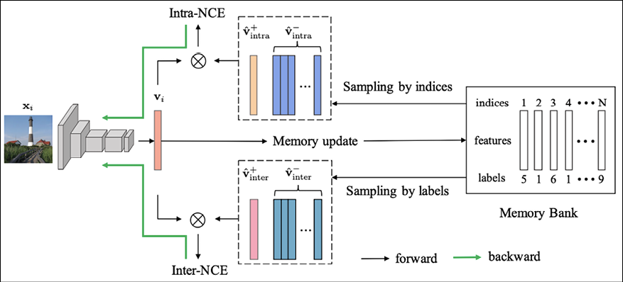
Figure 10.10: Architecture of the InterCLR model. From the paper: Delving into Inter-Image Invariance for Unsupervised Visual Representation [18]

The InterCLR paper also addresses some special considerations around pseudo label maintenance, sampling strategy, and decision boundary design for the inter-image branch, which we will skip here in the interests of space. The InterCLR model shows many improvements over state-of-the-art intra-image invariance learning methods on multiple standard benchmarks.

Multiview coding

Multiview coding has become a mainstream CL method in recent years and involves constructing positive contrastive examples using two or more views of the same object. The objective is to maximize the mutual information between the representations of the multiple views of the data for positive examples and minimize it for negative examples. This requires the model to learn higher-level features whose influence spans multiple views.

AMDIM

Augmented Multiscale Deep InfoMax (AMDIM) [31] is a model for self-supervised representational learning based on an earlier local Deep InfoMax method, which attempts to maximize the mutual information between a global summary feature that depends on the entire input, and a collection of local features that are extracted from intermediate layers in the encoder. AMDIM extends DIM by predicting features across independently augmented features of each input and simultaneously across multiple scales, as well as using a more powerful encoder.

The paper also considers other ways of producing contrastive pairs, such as instance transformation and multimodal (discussed in the next section), but it is described here because it also considers constructing contrastive pairs using multiview coding. The model beats several benchmarks for self-supervised learning objectives.

CMC

The Contrastive Multiview Coding (CMC) [37] model is based on the idea that when an object is represented by multiple views, each of these views is noisy and incomplete, but important factors such as the physics, geometry, and semantics of the object are usually shared across all the views. The goal of CMC is to learn a compact representation of the object that captures these important factors. CMC achieves this by using CL to learn a representation such that views of the same scene map to nearby points, whereas views of different scenes map to distant points.

Multimodal models

The class of models covered in this section includes models that use paired inputs from two or more modalities of the same data. The input to such a model could be an image and a caption, a video and text, an audio clip and its transcript, etc. These models learn a joint embedding across multiple modalities. In this class of models, we will cover the CLIP [6] and CodeSearchNet [13] models as examples.

Another class of multimodal models is frameworks that can be used to do self-supervised learning across multiple modalities. The Data2Vec [7] model is an example of such a model.

CLIP

The CLIP model [6] learns image representations by learning to predict which image goes with which caption. It is pretrained with 400 million image-text pairs from the internet. After pretraining, the model can use natural language queries to refer to learned visual concepts. CLIP can be used in zero-shot mode for downstream tasks such as image classification, text-to-image, and image-to-image image search. The model is competitive for natural images with a fully supervised baseline without the need for any additional fine-tuning. For example, CLIP can match the accuracy of the original ResNet50 on ImageNet in zero-shot mode, i.e., without additional fine-tuning. CLIP can also be fine-tuned with specialized image datasets for specific downstream tasks, such as learning visual representations for satellite imagery or tumor detection.

Figure 10.11 shows the architecture of the CLIP model for training and inference. Both image and text encoders are transformer-based encoders. The objective of pretraining is to solve the task of predicting which text as a whole is paired with which image. Thus, given a batch of N image-text pairs, CLIP learns to predict which of the N x N possible image-text pairs across the batch actually occurred. CLIP learns a multi-modal joint embedding space by maximizing the cosine similarity of the image and text embeddings of the N real pairs in the batch while minimizing the cosine similarity of the rest of the N² - N incorrect pairs.

During inference, the input of one modality can be used to predict the output of the other, i.e., given an image, it can predict the image class as text:

Figure 10.11: Architecture of the CLIP model. From the paper: Learning Transferable Visual Models from Natural Language Supervision [34x]

The code snippet below demonstrates the CLIP model’s ability to compare images and text. Here, we take an image of two cats side by side and compare it to two text strings: "a photo of a cat" and "a photo of a dog". CLIP can compare the image with the two text strings and correctly determine that the probability that the image is similar to the string "a photo of a cat" is 0.995 as opposed to a probability of 0.005 for the image being similar to the string "a photo of a dog":

import tensorflow as tf
from PIL import Image
import requests
from transformers import CLIPProcessor, TFCLIPModel
model = TFCLIPModel.from_pretrained("openai/clip-vit-base-patch32")
processor = CLIPProcessor.from_pretrained("openai/clip-vit-base-patch32")
url = "http://images.cocodataset.org/val2017/000000039769.jpg"
image = Image.open(requests.get(url, stream=True).raw)
texts = ["a photo of a cat", "a photo of a dog"]
inputs = processor(text=texts, images=image, return_tensors="tf", padding=True)
outputs = model(**inputs)
logits_per_image = outputs.logits_per_image
probs = tf.nn.softmax(logits_per_image, axis=1)
print(probs.numpy())

The CLIP model does this by projecting both text and image to a single embedding space. Using this common embedding approach, CLIP is also able to compute the similarity between two images and a text. It also offers the ability to extract encodings of text and images.

CodeSearchNet

The CodeSearchNet model [13] uses code snippets representing functions or methods in multiple programming languages (Go, Java, JavaScript, Python, PHP, and Ruby), and pairs them with (manually augmented) natural language comments describing the code to create positive examples. The corpus consists of approximately 2 million code-documentation pairs across all the different languages. As with CLIP, the goal of the CodeSearchNet model is to learn a joint embedding space of code and documentation, which can then be queried to return the appropriate code snippet (functions or methods) that satisfy some natural language query. The code and the natural language query are encoded using two separate encoders, and the model tries to learn a joint embedding that maximizes the inner product of the code and query encodings for positive pairs and minimizes it for negative pairs.

Data2Vec

Data2Vec [7] is a little different in that it proposes a common framework to do self-supervised learning across multiple modalities. It uses masked prediction to apply the same learning method for either speech, language, or computer vision. The core idea is to predict latent representations of the full input based on a masked view of the input. Instead of predicting modality-specific targets such as words, visual tokens, etc., it predicts contextualized latent representations that contain information for the entire input. It uses a teacher-student architecture – first, a representation of the full input data is built, which serves as the target for the learning task (teacher mode). Then a masked version of the input sample is encoded, with which the full data representation is predicted (student mode). The teacher’s parameters are updated using exponentially decaying average weights of the student. At the end of the training, the teacher’s weights are used as the learned embedding.

Experiments using this framework against major benchmarks in speech recognition, image classification, and natural language understanding show either state-of-the-art performance or competitive performance to popular approaches:

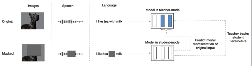
Figure 10.12: Architecture of the Data2Vec model. From the paper: data2vec: A General Framework for Self-supervised Learning in Speech, Vision and Language [7]

Pretext tasks

Pretext tasks are tasks that self-supervised learning models attempt to solve by leveraging some pattern inherent in the unlabeled data they train on. Such tasks are not necessarily useful in and of themselves, but they help the system learn a useful latent representation, or embeddings, that can then be used, either as-is or after fine-tuning, on some other downstream tasks. Training to solve pretext tasks usually happens as a precursor to building the actual model, and for that reason, it is also referred to as pretraining.

Almost all the techniques we have discussed in this chapter have been pretext tasks. While some tasks may end up being useful in and of themselves, such as colorization or super-resolution, they also result in embeddings that end up learning the semantics of the data distribution of the unlabeled data that it was trained on, in the form of learned weights. These weights can then be applied to downstream tasks.

This is not a new concept – for example, the Word2Vec algorithm, which is widely used for finding “synonyms,” is based on an embedding space where words used in similar contexts cluster together. It is trained using either the skip-gram or CBOW algorithm, which attempt to predict a context word given a word, or vice versa. Neither of these objectives are useful in and of themselves, but in the process, the network ends up learning a good latent representation of the words in the input data. This representation can then be directly used to find “synonyms” for words or do word analogies, as well as being used to produce useful vector representations of words and sequences of words (such as sentences and documents) for downstream tasks, such as text classification or sentiment analysis.

The biggest advantage of pretext tasks is that the training of models for downstream tasks can be done with relatively smaller amounts of labeled data. The model learns a lot about the domain (the broad strokes) based on solving the pretext task using large quantities of readily available unlabeled data. It requires relatively smaller amounts of labeled data to learn to solve more specific downstream tasks based on what it already knows about the domain. Because labeled data is hard to come by and expensive to create, this two-step approach can often make some machine learning models possible, if not more practical.

Summary

In this chapter, we saw various self-supervised strategies for leveraging data to learn the data distribution in the form of specialized embedding spaces, which in turn can be used for solving downstream tasks. We have looked at self-prediction, contrastive learning, and pretext tasks as specific approaches for self-supervision.

In the next chapter, we will look at reinforcement learning, an approach that uses rewards as a feedback mechanism to train models for specific tasks.

References

1. Aaron van den Oord, Nal Kalchbrenner, and Koray Kavucuoglu (2016). Pixel Recurrent Neural Networks Proceedings MLR Press: http://proceedings.mlr.press/v48/oord16.pdf
2. Aaron van den Oord, Yazhe Li, and Oriol Vinyals. Representation Learning with Contrastive Predictive Coding. Arxiv Preprint, arXiv 1807.03748 [cs.LG]: https://arxiv.org/pdf/1807.03748.pdf
3. Aaron van den Oord, et al. (2016). WaveNet: A Generative Model for Raw Audio. Arxiv Preprint, arXiv:1609.03499v2 [cs.SD]: https://arxiv.org/pdf/1609.03499.pdf
4. Abe Fetterman and Josh Albrecht. (2020). Understanding Self-Supervised and Contrastive Learning with “Bootstrap your Own Latent” (BYOL). Blog post: https://generallyintelligent.ai/blog/2020-08-24-understanding-self-supervised-contrastive-learning/
5. Aditya Ramesh, et al. Zero Shot Text to Image generation. Arxiv Preprint, arXiv 2102.12092v2 [cs.CV]: https://arxiv.org/pdf/2102.12092.pdf
6. Alec Radford, et al. (2021). Learning Transferable Visual Models from Natural Language Supervision. Proceedings of Machine Learning Research (PMLR): http://proceedings.mlr.press/v139/radford21a/radford21a.pdf
7. Alexei Baevsky, et al. (2022). data2vec: A General Framework for Self-Supervised Learning in Speech, Vision and Language. Arxiv Preprint, arXiv 2202.03555v1 [cs.LG]: https://arxiv.org/pdf/2202.03555.pdf
8. Carl Doersch, Abhinav Gupta and Alexei Efros. (2015). Unsupervised Visual Representation by Context Prediction. International Conference on Computer Vision (ICCV): https://www.cv-foundation.org/openaccess/content_iccv_2015/papers/Doersch_Unsupervised_Visual_Representation_ICCV_2015_paper.pdf
9. Chuan Li. (2020). OpenAI’s GPT-3 Language Model – a Technical Overview. LambdaLabs Blog post: https://lambdalabs.com/blog/demystifying-gpt-3/
10. Deepak Pathak, et al. (2016). Context Encoders: Feature Learning by Inpainting: https://openaccess.thecvf.com/content_cvpr_2016/papers/Pathak_Context_Encoders_Feature_CVPR_2016_paper.pdf
11. Florian Schroff, Dmitry Kalenichenko and James Philbin. (2025). FaceNet: A Unified Embedding for Face Recognition and Clustering. ArXiv Preprint, arXiv 1503.03832 [cs.CV]: https://arxiv.org/pdf/1503.03832.pdf
12. Gustav Larsson, Michael Maire and Gregory Shakhnarovich. (2017). Colorization as a Proxy Task for Visual Understanding: https://openaccess.thecvf.com/content_cvpr_2017/papers/Larsson_Colorization_as_a_CVPR_2017_paper.pdf
13. Hamel Husain, et al. (2020). CodeSearchNet Challenge: Evaluating the State of Semantic Code Search. Arxiv Preprint, arXiv: 1909.09436 [cs.LG]: https://arxiv.org/pdf/1909.09436.pdf
14. Hanting Chen, et al. (2021). Pre-trained Image Processing Transformer. Conference on Computer Vision and Pattern Recognition (CVPR): https://openaccess.thecvf.com/content/CVPR2021/papers/Chen_Pre-Trained_Image_Processing_Transformer_CVPR_2021_paper.pdf
15. Hyun Oh Song, Yu Xiang, Stefanie Jegelka and Silvio Savarese. (2015). Deep Metric Learning via Lifted Structured Feature Embedding. Arxiv Preprint, arXiv 1511.06452 [cs.CV]: https://arxiv.org/pdf/1511.06452.pdf
16. Jacob Devlin, et al. (2019). BERT: Pre-training of Deep Bidirectional Transformers for Language Understanding. Arxiv Preprint, arXiv: 1810.04805v2 [cs.CL]: https://arxiv.org/pdf/1810.04805.pdf
17. Jean-Bastien Grill, et al. (2020). Bootstrap your own latent: A new approach to self-supervised learning. Arxiv Preprint, arXiv 2006.07733 [cs.LG]: https://arxiv.org/pdf/2006.07733.pdf
18. Jiahao Xie, et al. (2021). Delving into Inter-Image Invariance for Unsupervised Visual Representations. Arxiv Preprint, arXiv: 2008.11702 [cs.CV]: https://arxiv.org/pdf/2008.11702.pdf
19. Joshua Robinson, Ching-Yao Chuang, Suvrit Sra and Stefanie Jegelka. (2021). Contrastive Learning with Hard Negative Samples. Arxiv Preprint, arXiv 2010.04592 [cs.LG]: https://arxiv.org/pdf/2010.04592.pdf
20. Jure Zobontar, et al. (2021). Barlow Twins: Self-Supervised Learning via Redundancy Reduction. Arxiv Preprint, arXiv 2103.03230 [cs.CV]: https://arxiv.org/pdf/2103.03230.pdf
21. Kihyuk Sohn. (2016). Improved Deep Metric Learning with Multi-class N-pair Loss Objective. Advances in Neural Information Processing Systems: https://proceedings.neurips.cc/paper/2016/file/6b180037abbebea991d8b1232f8a8ca9-Paper.pdf
22. Lilian Weng and Jong Wook Kim. (2021). Self-supervised Learning: Self Prediction and Contrastive Learning. NeurIPS Tutorial: https://neurips.cc/media/neurips-2021/Slides/21895.pdf
23. Lilian Weng. (Blog post 2021). Contrastive Representation Learning: https://lilianweng.github.io/posts/2021-05-31-contrastive/
24. Mathilde Caron, Piotr Bojanowsky, Armand Joulin and Matthijs Douze. (2019). Deep Clustering for Unsupervised Learning of Visual Features. Arxiv Preprint, arXiv: 1807.05520 [cs.CV]: https://arxiv.org/pdf/1807.05520.pdf
25. Mathilde Caron, et al. (2020). Unsupervised Learning of Visual Features by Contrasting Cluster Assignments. Arxiv Preprint, arXiv: 2006.099882 [cs.CV]: https://arxiv.org/pdf/2006.09882.pdf
26. Mehdi Noroozi and Paolo Favaro. (2016). Unsupervised Learning of Visual Representations by solving Jigsaw Puzzles. European Conference on Computer Vision: https://link.springer.com/chapter/10.1007/978-3-319-46466-4_5
27. Michael Gutmann, Aapo Hyvarinen. (2010). Noise-contrastive estimation: A new estimation principle for unnormalized statistical models. Proceedings of Machine Learning Research (PMLR): http://proceedings.mlr.press/v9/gutmann10a/gutmann10a.pdf
28. Nal Kalchbrenner, et al. (2018). Efficient Neural Audio Synthesis. Proceedings MLR Press: http://proceedings.mlr.press/v80/kalchbrenner18a/kalchbrenner18a.pdf
29. Pascal Vincent, et al. (2010). Stacked Denoising Autoencoders: Learning Useful Representations in a Deep Network with a Local Denoising Criterion. Journal of Machine Learning Research (JMLR): https://www.jmlr.org/papers/volume11/vincent10a/vincent10a.pdf?ref=https://githubhelp.com
30. Patrick Esser, Robin Rombach and Bjorn Ommer. (2021). Taming Transformers for High-Resolution Image Synthesis. Computer Vision and Pattern Recognition (CVPR): https://openaccess.thecvf.com/content/CVPR2021/papers/Esser_Taming_Transformers_for_High-Resolution_Image_Synthesis_CVPR_2021_paper.pdf
31. Philip Bachman, R Devon Hjelm and William Buchwalter. (2019). Learning Representations by Maximizing Mutual Information across Views. Advances in Neural Information Processing Systems (NeurIPS): https://proceedings.neurips.cc/paper/2019/file/ddf354219aac374f1d40b7e760ee5bb7-Paper.pdf
32. Prafulla Dhariwal, et al. (2020). Jukebox: A Generative Model for Music. Arxiv Preprint, arXiv 2005.00341v1 [eess.AS]: https://arxiv.org/pdf/2005.00341.pdf
33. Ruslan Salakhutdinov and Geoff Hinton. (2007). Learning a Nonlinear Embedding by Preserving Class Neighborhood Structure. Proceedings of Machine Learning Research (PMLR): http://proceedings.mlr.press/v2/salakhutdinov07a/salakhutdinov07a.pdf
34. Spyros Gidaris, Praveer Singh and Nicos Komodakis. (2018). Unsupervised Representation Learning by Predicting Image Rotations. Arxiv Preprint, arXiv 1803.07728v1 [cs.CV]: https://arxiv.org/pdf/1803.07728.pdf
35. Sumit Chopra, et al. (2005). Learning a Similarity Metric Discriminatively, with application to Face Verification. IEEE Computer Society: http://www.cs.utoronto.ca/~hinton/csc2535_06/readings/chopra-05.pdf
36. Ting Chen, Simon Kornblith, Mohammed Norouzi and Geoffrey Hinton. (2020). A Simple Framework for Contrastive Learning. Arxiv Preprint, arXiv 2002.05709 [cs.LG]: https://arxiv.org/pdf/2002.05709.pdf
37. Yonglong Tian, Dilip Krishnan and Philip Isola. (2020). Contrastive Multiview Coding. Arxiv Preprint, arXiv: 1906.05849 [cs.CV]: https://arxiv.org/pdf/1906.05849.pdf?ref=https://githubhelp.com
38. Zhilin Yang, et al. (2019). XLNet: Generalized Autoregressive Pre-training for Language Understanding: https://proceedings.neurips.cc/paper/2019/file/dc6a7e655d7e5840e66733e9ee67cc69-Paper.pdf
39. Prompt Engineering. (7th July 2022). Wikipedia, Wikimedia Foundation: https://en.wikipedia.org/wiki/Prompt_engineering

Join our book’s Discord space

Join our Discord community to meet like-minded people and learn alongside more than 2000 members at: https://packt.link/keras