6

Transformers

The transformer-based architectures have become almost universal in Natural Language Processing (NLP) (and beyond) when it comes to solving a wide variety of tasks, such as:

• Neural machine translation
• Text summarization
• Text generation
• Named entity recognition
• Question answering
• Text classification
• Text similarity
• Offensive message/profanity detection
• Query understanding
• Language modeling
• Next-sentence prediction
• Reading comprehension
• Sentiment analysis
• Paraphrasing

and a lot more.

In less than four years, when the Attention Is All You Need paper was published by Google Research in 2017, transformers managed to take the NLP community by storm, breaking any record achieved over the previous thirty years.

Transformer-based models use the so-called attention mechanisms that identify complex relationships between words in each input sequence, such as a sentence. Attention helped resolve the challenge of encoding “pairwise correlations”—something that its “predecessors,” such as LSTM RNNs and even CNNS, couldn’t achieve when modeling sequential data, such as text.

Models—such as BERT, T5, and GPT (covered in more detail later in this chapter)—now constitute the state-of-the-art fundamental building blocks for new applications in almost every field, from computer vision to speech recognition, translation, or protein and coding sequences. Attention has also been applied in reinforcement learning for games: in DeepMind’s AlphaStar (https://rdcu.be/bVI7G and https://www.deepmind.com/blog/alphastar-grandmaster-level-in-starcraft-ii-using-multi-agent-reinforcement-learning), observations of player and opponent StarCraft game units were processed with self-attention, for example. For this reason, Stanford has recently introduced the term “foundation models” to define a set of Large Language Models (LLMs) based on giant pretrained transformers.

This progress has been made thanks to a few simple ideas, which we are going to review in the next few sections.

You will learn:

• What transformers are
• How they evolved over time
• Some optimization techniques
• Dos and don’ts
• What the future will look like

Let’s start turning our attention to transformers. You will be surprised to discover that attention indeed is all you need!

Architecture

Even though a typical transformer architecture is usually different from that of recurrent networks, it is based on several key ideas that originated in RNNs. At the time of writing this book, the transformer represents the next evolutionary step of deep learning architectures related to texts and any data that can be represented as sequences, and as such, it should be an essential part of your toolbox.

The original transformer architecture is a variant of the encoder-decoder architecture, where the recurrent layers are replaced with (self-)attention layers. The transformer was initially proposed by Google in the seminal paper titled Attention Is All You Need by Ashish Vaswani, Noam Shazeer, Niki Parmar, Jakob Uszkoreit, Llion Jones, Aidan N. Gomez, Lukasz Kaiser, and Illia Polosukhin, 2017, https://arxiv.org/abs/1706.03762, to which a reference implementation was provided, which we will refer to throughout this discussion.

The architecture is an instance of the encoder-decoder models that have been popular since 2014-2015 (such as Sequence to Sequence Learning with Neural Networks by Sutskever et al. (2014), https://arxiv.org/abs/1409.3215). Prior to that, attention had been used together with Long-Short-Term Memory (LSTM) and other RNN (Recurrent Neural Network) models discussed in a previous chapter. Attention was introduced in 2014 in Neural Machine Translation by Jointly Learning to Align and Translate by Bahdanau et al., https://arxiv.org/abs/1409.0473, and applied to neural machine translation in 2015 in Effective Approaches to Attention-based Neural Machine Translation by Luong et al., https://arxiv.org/abs/1508.04025, and there have been other combinations of attention with other types of models.

In 2017, the first transformer demonstrated that you could remove LSTMs from Neural Machine Translation (NMT) models and use the so-called (self-)attention blocks (hence the paper title Attention Is All You Need).

Key intuitions

Let’s start by defining some concepts that will be useful later on in this chapter. The innovation introduced with the transformer in 2017 is based on four main key ideas:

• Positional encoding
• Attention
• Self-attention
• Multi-head (self-)attention

In the next sections, we will discuss them in greater detail.

Positional encoding

RNNs keep the word order by processing words sequentially. The advantage of this approach is simplicity, but one of the disadvantages is that this makes parallelization hard (training on multiple hardware accelerators). If we want to effectively leverage highly parallel architectures, such as GPUs and TPUs, we’d need an alternative way to represent ordering.

The transformer uses a simple alternative order representation called positional encoding, which associates each word with a number representing its position in the text. For instance:

[("Transformers", 1), ("took", 2), ("NLP", 3), ("by", 4), ("storm", 5)]

The key intuition is that enriching transformers with a position allows the model to learn the importance of the position of each token (a word in the text/sentence). Note that positional encoding existed before transformers (as discussed in the chapter on RNNs), but this intuition is particularly important in the context of creating transformer-based models. After (absolute) positional encoding was introduced in the original transformer paper, there have been other variants, such as relative positional encoding (Self-Attention with Relative Position Representations by Shaw et al., 2018, https://arxiv.org/abs/1803.02155, and rotary positional encoding (RoFormer: Enhanced Transformer with Rotary Position Embedding by Su et al., 2021, https://arxiv.org/abs/2104.09864).

Now that we have defined positional encoding, let’s turn our attention to the attention mechanism.

Attention

Another crucial ingredient of the transformer recipe is attention. This mechanism was first introduced in the context of machine translation in 2014 by Bahdanou et al. in Neural Machine Translation by Jointly Learning to Align and Translate by Dzmitry Bahdanau, KyungHyun Cho, and Yoshua Bengio, https://arxiv.org/pdf/1409.0473.pdf. Some research papers also attribute the idea behind attention to Alex Graves’ Generating Sequences with Recurrent Neural Networks, which dates back to 2013, https://arxiv.org/pdf/1308.0850.pdf.

This ingredient—this key idea—has since become a part of the title of the first transformer paper, Attention is All You Need. To get a high-level overview, let’s consider this example from the paper that introduced attention:

The agreement on the European Economic Area was signed in August 1992.

In French, this can be translated as:

L’accord sur la zone économique européenne a été signé en août 1992.

The initial attempts to perform automatic machine translation back in the early 80s were based on the sequential translation of each word. This approach was very limiting because the text structure can change from a source language to a target language in many ways. For instance, some words in the French translation can have a different order: in English, adjectives usually precede nouns, like in “European Economic Area,” whereas in French, adjectives can go after nouns—”la zone économique européenne.” Moreover, unlike in English, the French language has gendered words. So, for example, the adjectives “économique” and “européenne” must be in their feminine form as they belong to the feminine noun “la zone.”

The key intuition behind the attention approach is to build a text model that “looks at” every single word in the source sentence when translating words into the output language. In the original 2017 transformer paper, the authors point out that the cost of doing this is quadratic, but the gain achieved in terms of more accurate translation is considerable. More recent works reduced this initial quadratic complexity, such as the Fast Attention Via positive Orthogonal Random (FAVOR+) features from the Rethinking Attention with Performers paper by Choromanski et al. (2020) from Google, DeepMind, the University of Cambridge, and the Alan Turing Institute.

Let’s go over a nice example from that original attention paper by Bahdanou et al. (2014):

Figure 6.1: An example of attention for the English sentence “The agreement on the European Economic Area was signed in August 1992.” The plot visualizes “annotation weights”—the weights associated with the annotations. Source: “Neural Machine Translation by Jointly Learning to Align and Translate” by Bahdanau et al. (2014) (https://arxiv.org/abs/1409.0473)

Using the attention mechanism, the neural network can learn a heatmap of each source English word in relation to each target French word. Note that relationships are not only on the diagonal but might spread across the whole matrix. For instance, when the model outputs the French word “européenne,” it will pay a lot of attention to the input words “European” and “Economic.” (In Figure 6.1, this corresponds to the diagonal and the adjacent cell.) The 2014 attention paper by Bahdanou et al. demonstrated that the model (which used an RNN encoder-decoder framework with attention) can learn to align and attend to the input elements without supervision, and, as Figure 6.1 shows, translate the input English sentences into French. And, of course, the larger the training set is, the greater the number of correlations that the attention-based model can learn.

In short, the attention mechanism can access all previous words and weigh them according to a learned measure of relevancy. This way, attention can provide relevant information about tokens located far away in the target sentence.

Now, we can focus on another key ingredient of the transformer—”self-attention.”

Self-attention

The third key idea popularized by the original transformer paper is the use of attention within the same sentence in the source language—self-attention. With this mechanism, neural networks can be trained to learn the relationships among all words (or other elements) in each input sequence (such as a sentence) irrespective of their positions before focusing on (machine) translation. Self-attention can be attributed to the idea from the 2016 paper called Long Short-Term Memory-Networks for Machine Reading by Cheng et al., https://arxiv.org/pdf/1601.06733.pdf.

Let’s go through an example with the following two sentences:

“Server, can I have the check?”

“Looks like I just crashed the server.”

Clearly, the word “server” has a very different meaning in either sentence and self-attention can understand each word considering the context of the surrounding words. Just to reiterate, the attention mechanism can access all previous words and weigh them according to a learned measure of relevancy. Self-attention provides relevant information about tokens located far away in the source sentence.

Multi-head (self-)attention

The original transformer performs a (self-)attention function multiple times. A single set of the so-called weight matrices (which are covered in detail in the How to compute Attention section) is named an attention head. When you have several sets of these matrices, you have multiple attention heads. The multi-head (self-)attention layer usually has several parallel (self-)attention layers. Note that the introduction of multiple heads allows us to have many definitions of which word is “relevant” to each other. Plus, all these definitions of relevance can be computed in parallel by modern hardware accelerators, thus speeding up the computation.

Now that we have gone through the high-level definitions of the key ingredients of the transformers, let’s deep dive into how to compute the attention mechanism.

How to compute attention

In the original transformer, the self-attention function is computed by using the so-called scaled dot-product units. The authors of the 2017 paper even called their attention method Scaled Dot-Product Attention. You might remember from high school studies that the dot-product between two vectors provides a good sense of how “close” the vectors are.

Each input token sequence (for example, of a sentence) embedding that passes into the transformer (encoder and/or decoder) produces attention weights (covered in detail below) that are simultaneously calculated between every sequence element (such as a word). The output results in embeddings produced for every token containing the token itself together with every other relevant token weighted by its relative attention weight.

The attention layer transforms the input vectors into query, key, and value matrices, which are then split into attention heads (hence, multi-head attention):

• The query word can be interpreted as the word for which we are calculating the attention function.
• The key and value words are the words to which we are paying attention.

The dot-product (explained further below) tells us the similarity between words. If the vectors for two words are more aligned, the attention score will be higher. The transformer will learn the weights in such a way that if two words in a sentence are relevant to each other, then their word vectors will be aligned.

Each attention layer learns three weight matrices:

• The query weights W_Q
• The key weights W_K
• The value weights W_V

For each word i, an input word embedding x_i is computed producing:

• A query vector q_i = x_iW_Q
• A key vector k_i = x_iW_K
• A value vector v_i = x_iW_V

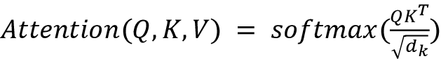
Given the query and the corresponding key vectors, the following dot-product formula produces the attention weight in the original transformer paper:

where:

• a_i,j is the attention from word i to a word j.
• . is the dot-product of the query with keys, which will give a sense of how “close” the vectors are.

Note that the attention unit for word i is the weighted sum of the value vectors of all words, weighted by a_i,j, the attention from word i to a word j.

Now, to stabilize gradients during the training, the attention weights are divided by the square root of the dimension of the key vectors .

Then, the results are passed through a softmax function to normalize the weight. Note that the attention function from a word i to a word j is not the same as the attention from word j to a word i.

Note that since modern deep learning accelerators work well with matrices, we can compute attention for all words using large matrices.

Define q_i, k_i, v_i (where i is the ith row) as matrices Q, K, V, respectively. Then, we can summarize the attention function as an attention matrix:

In this section, we discussed how to compute the attention function introduced in the original transformer paper. Next, let’s discuss the encoder-decoder architecture.

Encoder-decoder architecture

Similar to the seq2seq models, (Sequence to Sequence Learning with Neural Networks by Ilya Sutskever, Oriol Vinyals, Quoc V. Le (2014)) described in Chapter 5, Recurrent Neural Networks, the original transformer model also used an encoder-decoder architecture:

• The encoder takes the input (source) sequence of embeddings and transforms it into a new fixed-length vector of input embeddings.
• The decoder takes the output embeddings vector from the encoder and transforms it into a sequence of output embeddings.
• Both the encoder and the decoder consist of several stacked layers. Each encoder and decoder layer is using the attention mechanism described earlier.

We’ll learn about the transformer architecture in much more detail later in this section.

Since the introduction of the transformer architecture, other newer networks have used only the encoder or the decoder components (or both), which are discussed in the Categories of transformers section of this chapter.

Next, let’s briefly go over the other components of the original transformer—the residual and normalization layers.

Residual and normalization layers

Typically, transformer-based networks reuse other existing state-of-the-art machine learning methodologies, such as attention mechanisms. You shall therefore not be surprised if both encoder and decoder layers combine neural networks with residual connections (Deep Residual Learning for Image Recognition by He et al., 2016, https://arxiv.org/abs/1512.03385) and normalization steps (Layer Normalization by Ba et al., 2016, https:/arxiv.org/abs/1607.06450).

OK, we now have all the key ingredients to deep dive into transformers.

An overview of the transformer architecture

Now that we have covered some of the key concepts behind the original transformer, let’s deep dive into the architecture introduced in the seminal 2017 paper. Note that transformer-based models are usually built by leveraging various attention mechanisms without using RNNs. This is also a consequence of the fact that attention mechanisms themselves can match and outperform RNN (encoder-decoder) models with attention. That’s why the seminal paper was titled Attention is all You Need.

Figure 6.2 shows a seq2seq network with RNNs and attention, and compares it to the original transformer network.

The transformer is similar to seq2seq with an attention model in the following ways:

• Both approaches work with source (inputs) and target (output) sequences.
• Both use an encoder-decoder architecture, as mentioned before.
• The output of the last block of the encoder is used as a context—or thought vector—for computing the attention function in the decoder.
• The target (output) sequence embeddings are fed into dense (fully connected) blocks, which convert the output embeddings to the final sequence of an integer form:

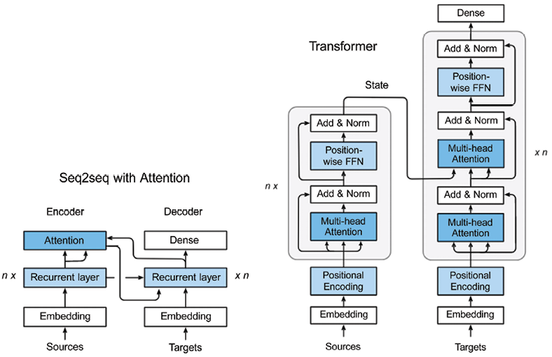
Figure 6.2: Flow of data in (a) seq2seq + Attention, and (b) Transformer architecture. Image Source: Zhang, et al.

And the two architectures differ in the following ways:

• The seq2seq network uses the recurrent and attention layers in the encoder, and the recurrent layer in the decoder.

  The transformer replaced those layers with so-called transformer blocks (a stack of N identical layers), as Figure 6.2 demonstrates:

  • In the encoder, the transformer block consists of a sequence of sub-layers: a multi-head (self-)attention layer and a position-wise feedforward layer. Each of those two layers has a residual connection, followed by a normalization layer.
  • In the decoder, the transformer block contains a variant of a multi-head (self-)attention layer with masking—a masked multi-head self-attention—and a feedforward layer like in the encoder (with identical residual connections and normalization layers). Masking helps prevent positions from attending into the future. Additionally, the decoder contains a second multi-head (self-)attention layer which computes attention over the outputs of the encoder’s transformer blockmasking is covered in more detail later in this section.)

• In the seq2seq with attention network, the encoder state is passed to the first recurrent time step as with the seq2seq with attention network.

  In the transformer, the encoder state is passed to every transformer block in the decoder. This allows the transformer network to work in parallel across time steps since there is no longer a temporal dependency as with the seq2seq networks.

  The last decoder is followed by a final linear transformation (a dense layer) with a softmax function to produce the output (next-token) probabilities.

• Because of the parallelism referred to in the previous point, an encoding layer is added to provide positional information to distinguish the position of each element in the transformer network sequence (positional encoding layer). This way, the first encoder takes the positional information and embeddings of the input sequence as inputs, rather than only encodings, thus allowing taking positional information into account.

Let’s walk through the process of data flowing through the transformer network. Later in this chapter, we will use TensorFlow with the Keras API to create and train a transformer model from scratch:

1. As part of data preprocessing, the inputs and the outputs are tokenized and converted to embeddings.
2. Next, positional encoding is applied to the input and output embeddings to have information about the relative position of tokens in the sequences. In the encoder section:
   • As per Figure 6.2, the encoder side consists of an embedding and a positional encoding layer, followed by six identical transformer blocks (there were six “layers” in the original transformer). As we learned earlier, each transformer block in the encoder consists of a multi-head (self-)attention layer and a position-wise feedforward layer.

   We have already briefly seen that self-attention is the process of attending to parts of the same sequence. When we process a sentence, we might want to know what other words are most aligned with the current one.

   • The multi-head attention layer consists of multiple (eight in the reference implementation contained in the seminal paper) parallel self-attention layers. Self-attention is carried out by constructing three vectors Q (query), K (key), and V (value), out of the input embedding. These vectors are created by multiplying the input embedding with three trainable weight matrices W_Q, W_K, and W_V. The output vector Z is created by combining K, Q, and V at each self-attention layer using the following formula. Here, d_K refers to the dimension of the K, Q, and V vectors (64 in the reference implementation contained in the seminal paper):

   

   • The multi-head attention layer will create multiple values for Z (based on multiple trainable weight matrices W_Q, W_K, and W_V at each self-attention layer), and then concatenate them for inputs into the position-wise feedforward layer.
   • The inputs to the position-wise feedforward layer consist of embeddings for the different elements in the sequence (or words in the sentence), attended via self-attention in the multi-head attention layer. Each token is represented internally by a fixed-length embedding vector (512 in the reference implementation introduced in the seminal paper). Each vector is run through the feedforward layer in parallel. The outputs of the FFN are the inputs to (or fed into) the multi-head attention layer in the following transformer block. In the last transformer block of the encoder, the outputs are the context vector that is passed to the decoder.
   • Both the multi-head attention and position-wise FFN layers send out not only the signal from the previous layer but also a residual signal from their inputs to their outputs. The outputs and residual inputs are passed through a layer-normalization step, and this is shown in Figure 6.2 as the “Add & Norm” layer.
   • Since the entire sequence is consumed in parallel on the encoder, the information about the positions of individual elements gets lost. To compensate for this, the input embeddings are augmented with a positional embedding, which is implemented as a sinusoidal function without learned parameters. The positional embedding is added to the input embedding.

3. Next, let’s walk through how the data flows through the decoder:
   • The output of the encoder results in a pair of attention vectors K and V, which are sent in parallel to all the transformer blocks in the decoder. The transformer block in the decoder is similar to that in the encoder, except that it has an additional multi-head attention layer to handle the attention vectors from the encoder. This additional multi-head attention layer works similarly to the one in the encoder and the one below it, except that it combines the Q vector from the layer below it and the K and Q vectors from the encoder state.
   • Similar to the seq2seq network, the output sequence generates one token at a time, using the input from the previous time step. As for the input to the encoder, the input to the decoder is also augmented with a positional embedding. Unlike the encoder, the self-attention process in the decoder is only allowed to attend to tokens at previous time points. This is done by masking out tokens at future time points.
   • The output of the last transformer block in the decoder is a sequence of low-dimensional embeddings (512 for reference implementation in the seminal paper as noted earlier). This is passed to the dense layer, which converts it into a sequence of probability distributions across the target vocabulary, from which we generate the most probable word either greedily or by a more sophisticated technique such as beam search.

Figure 6.3 shows the transformer architecture covering everything that’s just been described:

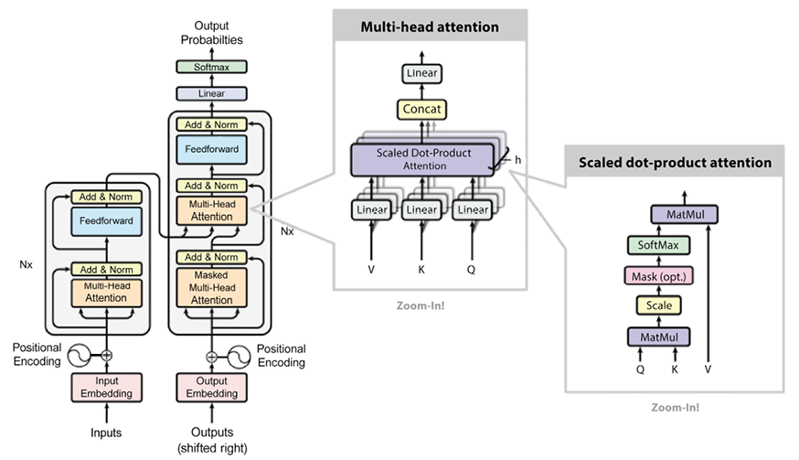
Figure 6.3: The transformer architecture based on original images from “Attention Is All You Need” by Vaswani et al. (2017)

Training

Transformers are typically trained via semi-supervised learning in two steps:

1. First, an unsupervised pretraining, typically on a very large corpus.
2. Then, a supervised fine-tuning on a smaller labeled dataset.

Both pretraining and fine-tuning might require significant resources in terms of GPU/TPU, memory, and time. This is especially true, considering that large language models (in short, LLMs) have an increasing number of parameters as we will see in the next section.

Sometimes, the second phase has a very limited set of labeled data. This is the so-called few-shot learning, which considers making predictions based on a limited number of samples.

Transformers’ architectures

In this section, we have provided a high-level overview of both the most important architectures used by transformers and of the different ways used to compute attention.

Categories of transformers

In this section, we are going to classify transformers into different categories. The next paragraph will introduce the most common transformers.

Decoder or autoregressive

A typical example is a GPT (Generative Pre-Trained) model, which you can learn more about in the GPT-2 and GPT-3 sections later in this chapter, or refer to https://openai.com/blog/language-unsupervised). Autoregressive models use only the decoder of the original transformer model, with the attention heads that can only see what is before in the text and not after with a masking mechanism used on the full sentence. Autoregressive models use pretraining to guess the next token after observing all the previous ones. Typically, autoregressive models are used for Natural Language Generation (NLG) text generation tasks. Other examples of autoregressive models include the original GPT, GPT-2, Transformer-XL, Reformer, and XLNet, which are covered later in this chapter.

Encoder or autoencoding

A typical example is BERT (Bidirectional Encoder Representations from Transformers), which is covered later in this chapter. Autoencoders correspond to the encoder in the original transformer model having access to the full input tokens with no masks. Autoencoding models use pretraining by masking/altering the input tokens and then trying to reconstruct the original sentence. Frequently, the models build a bidirectional representation of the full sentences. Note that the only difference between autoencoders and autoregressive is the pretraining phase, so the same architecture can be used in both ways. Autoencoders can be used for NLG, as well as for classification and many other NLP tasks. Other examples of autoencoding models, apart from BERT, include ALBERT, RoBERTa, and ELECTRA, which you can learn about later in this chapter.

Seq2seq

A typical example is T5 (Text-to-Text Transfer Transformer) and the original transformer. Sequence-to-sequence models use both the encoder and the decoder of the original transformer architecture. Seq2seq can be fine-tuned to many tasks such as translation, summarization, ranking, and question answering. Another example of a seq2seq model, apart from the original transformer and T5, is Multitask Unified Model (MUM).

Multimodal

A typical example is MUM. Multimodal models mix text inputs with other kinds of content (for example, images, videos, and audio).

Retrieval

A typical example is RETRO. Some models use document retrieval during (pre)training and inference. This is frequently a good strategy to reduce the size of the model and rapidly access memorized information saving on the number of used parameters.

Attention

Now that we have understood how to classify transformers, let’s focus on attention!

There is a wide variety of attention mechanisms, such as self-attention, local/hard attention, and global/soft attention, to name a few. Below, we’ll focus on some of the examples.

Full versus sparse

As discussed, the (scaled) dot-product attention from the original 2017 transformer paper is typically computed on a full squared matrix O(L²) where L is the length of the maximal considered sequence (in some configurations L = 512). The BigBird type of transformer, proposed by Google Research in 2020 and discussed in more detail later in this chapter, introduced the idea of using sparse attention by leveraging sparse matrices (based on the 2019 work by OpenAI’s Generating long sequences with sparse transformers by Child et al., https://arxiv.org/abs/1904.10509).

LSH attention

The Reformer introduced the idea of reducing the attention mechanism complexity with hashing—the model’s authors called it locality-sensitive hashing attention. The approach is based on the notion of using only the largest elements when softmax(QK^T) is computed. In other words, for each query only the keys that are close to q are computed. For computing closeness, several hash functions are computed according to local sensitive hashing techniques.

Local attention

Some transformers adopted the idea of having only a local window of context (e.g. a few tokens on the right and a few tokens on the left). The idea is that using fewer parameters allows us to consider longer sequences but with a limited degree of attention. For this reason, local attention is less popular.

Pretraining

As you have learned earlier, the original transformer had an encoder-decoder architecture. However, the research community understood that there are situations where it is beneficial to have only the encoder, or only the decoder, or both.

Encoder pretraining

As discussed, these models are also called auto-encoding and they use only the encoder during the pretraining. Pretraining is carried out by masking words in the input sequence and training the model to reconstruct the sequence. Typically, the encoder can access all the input words. Encoder-only models are generally used for classification.

Decoder pretraining

Decoder models are referred to as autoregressive. During pretraining, the decoder is optimized to predict the next word. In particular, the decoder can only access all the words positioned before a given word in the sequence. Decoder-only models are generally used for text generation.

Encoder-decoder pretraining

In this case, the model can use both the encoder and the decoder. Attention in the encoder can use all the words in the sequence, while attention in the decoder can only use the words preceding a given word in the sequence. Encoder-decoder has a large range of applications including text generation, translation, summarization, and generative question answer.

A taxonomy for pretraining tasks

It can be useful to organize pretraining into a taxonomy suggested by Pre-trained Models for Natural Language Processing: A Survey, Xipeng Qiu, 2020, https://arxiv.org/abs/2003.08271:

• Language Modeling (LM): For unidirectional LM, the task is to predict the next token. For bidirectional LM, the task is to predict the previous and next tokens.
• Masked Language Modeling (MLM): The key idea is to mask out some tokens from the input sentences. Then, the model is trained to predict the masked tokens given the non-masked tokens.
• Permuted Language Modeling (PLM): This is similar to LM, but a random permutation of input sequences is performed. Then, a subset of tokens is chosen as the target, and the model is trained to predict these targets.
• Denoising Autoencoder (DAE): Deliberately provide partially corrupted input. For instance, randomly sample input tokens and replace them with special [MASK] elements. Alternatively, randomly delete input tokens. Alternatively, shuffle sentences in random order. The task is to recover the original undistorted input.
• Contrastive Learning (CTL): The task is to learn a score function for text pairs by assuming that some observed pairs of text are more semantically similar than randomly sampled text. This class of techniques includes a number of specific techniques such as:
  • Deep InfoMax (DIM): Maximize mutual information between an input image representation and various local regions of the same image.
  • Replaced Token Detection (RTD): Predict whether an input token is replaced given its surroundings.
  • Next Sentence Prediction (NSP): The model is trained to distinguish whether two input sentences are contiguous in the training corpus.
  • Sentence Order Prediction (SOP): The same ideas as NSP with some additional signals: two consecutive segments are positive examples, and two swapped segments are negative examples.

In this section, we have briefly reviewed different pretraining techniques. The next section will review a selection of the most used transformers.

An overview of popular and well-known models

After the seminal paper Attention is All You Need, a very large number of alternative transformer-based models have been proposed. Let’s review some of the most popular and well-known ones.

BERT

BERT, or Bidirectional Encoder Representations from Transformers, is a language representation model developed by the Google AI research team in 2018. Let’s go over the main intuition behind that model:

1. BERT considers the context of each word from both the left and the right side using the so-called “bidirectional self-attention.”
2. Training happens by randomly masking the input word tokens, and avoiding cycles so that words cannot see themselves indirectly. In NLP jargon, this is called “fill in the blank.” In other words, the pretraining task involves masking a small subset of unlabeled inputs and then training the network to recover these original inputs. (This is an example of MLM.)
3. The model uses classification for pretraining to predict whether a sentence sequence S is before a sentence T. This way, BERT can understand relationships among sentences (“Next Sentence Prediction”), such as “does sentence T come after sentence S?” The idea of pretraining became a new standard for LLM.
4. BERT—namely BERT Large—became one of the first large language models with 24 transformer blocks, 1024-hidden layers, 16 self-attention heads, and 340M parameters. The model is trained on a large 3.3 billion words corpus.

BERT produced state-of-the-art results for 11 NLP tasks, including:

• GLUE score of 80.4%, a 7.6% absolute improvement from the previous best result.
• 93.2% accuracy on SQuAD 1.1 and outperforming human performance by 2%.

We will see GLUE and SQuAD metrics later in this chapter. If you want to know more, you can explore the following material:

• The original research paper: BERT: Pre-training of Deep Bidirectional Transformers for Language Understanding by Jacob Devlin, Ming-Wei Chang, Kenton Lee, Kristina Toutanova, 2018, https://arxiv.org/abs/1810.04805.
• The Google AI blog post: Open Sourcing BERT: State-of-the-Art Pre-training for Natural Language Processing, 2018, which discusses the advancement of the (then) state-of-the-art model for 11 NLP tasks (https://ai.googleblog.com/2018/11/open-sourcing-bert-state-of-art-pre.html.)
• An open source TensorFlow implementation and the pretrained BERT models are available at http://goo.gl/language/bert and from TensorFlow Model Garden at https://github.com/tensorflow/models/tree/master/official/nlp/modeling/models.
• A Colab notebook for BERT is available here: https://colab.research.google.com/github/tensorflow/tpu/blob/master/tools/colab/bert_finetuning_with_cloud_tpus.ipynb.
• BERT FineTuning with Cloud TPU: A tutorial that shows how to train the BERT model on Cloud TPU for sentence and sentence-pair classification tasks: https://cloud.google.com/tpu/docs/tutorials/bert.
• A Google blog post about applying BERT to Google Search to improve language understanding. According to Google, BERT “will help Search better understand one in 10 searches in the U.S. in English.” Moreover, the post mentions that “A powerful characteristic of these systems is that they can take learnings from one language and apply them to others. So we can take models that learn from improvements in English (a language where the vast majority of web content exists) and apply them to other languages.” (from Understanding search better than ever before): https://blog.google/products/search/search-language-understanding-bert/.

GPT-2

GPT-2 is a model introduced by OpenAI in Language Models Are Unsupervised Multitask Learners by Alec Radford, Jeffrey Wu, Rewon Child, David Luan, Dario Amodei, and Ilya Sutskever, https://openai.com/blog/better-language-models/, https://openai.com/blog/gpt-2-6-month-follow-up/, https://www.openai.com/blog/gpt-2-1-5b-release/, and https://github.com/openai/gpt-2.)

Let’s review the key intuitions:

• The largest of four model sizes was a 1.5 billion-parameter transformer with 48 layers trained on a new dataset called Webtext containing text from 45 million webpages.
• GPT-2 used the original 2017 transformer-based architecture and a modified version of the original GPT model (also developed by OpenAI) by Radford et al., 2018, Improving Language Understanding by Generative Pre-Training, https://openai.com/blog/language-unsupervised/, and https://cdn.openai.com/research-covers/language-unsupervised/language_understanding_paper.pdf).
• The research demonstrated that an LLM trained on a large and diverse dataset can perform well on a wide variety of NLP tasks, such as question answering, machine translation, reading comprehension, and summarization. Previously, the tasks had been typically approached with supervised learning on task-specific datasets. GPT-2 was trained in an unsupervised manner and performed well at zero-shot task transfer.
• Initially, OpenAI released only a smaller version of GPT-2 with 117 M parameters, “due to concerns about large language models being used to generate deceptive, biased, or abusive language at scale.” Then, the model was released: https://openai.com/blog/gpt-2-1-5b-release/.
• Interestingly enough, OpenAI developed an ML-based detection method to test whether an actor is generating synthetic texts for propaganda. The detection rates were ~95% for detecting 1.5B GPT-2-generated text: https://github.com/openai/gpt-2-output-dataset.

Similar to the original GPT from 2018, GPT-2 does not require the encoder part of the original transformer model – it uses a multi-layer decoder for language modeling. The decoder can only get information from the prior words in the sentence. It takes word vectors as input and produces estimates for the probability of the next word as output, but it is autoregressive, meaning that each token in the sentence relies on the context of the previous words. On the other hand, BERT is not autoregressive, as it uses the entire surrounding context all at once.

GPT-2 was the first LLM showing commonsense reasoning, capable of performing a number of NLP tasks including translation, question answering, and reading comprehension. The model achieved state-of-the-art results on 7 out of 8 tested language modeling datasets.

GPT-3

GPT-3 is an autoregressive language model developed by OpenAI and introduced in 2019 in Language Models are Few-Shot Learners by Tom B. Brown, et al., https://arxiv.org/abs/2005.14165. Let’s look at the key intuitions:

• GPT-3 uses an architecture and model similar to GPT-2 with a major difference consisting of the adoption of a sparse attention mechanism.
• For each task, the model evaluation has three different approaches:
  • Few-shot learning: The model receives a few demonstrations of the task (typically, less than one hundred) at inference time. However, no weight updates are allowed.
  • One-shot learning: The model receives only one demonstration and a natural language description of the task.
  • Zero-shot learning: The model receives no demonstration, but it has access only to a natural language description of the task.
• For all tasks, GPT-3 is applied without any gradient updates, complete with tasks and few-shot demonstrations specified purely via text interaction with the model.

The number of parameters the researchers trained GPT-3 with ranges from 125 million (GPT-3 Small) to 175 billion (GPT-3 175B). With no fine-tuning, the model achieves significant results on many NLP tasks including translation and question answering, sometimes surpassing state-of-the-art models. In particular, GPT-3 showed impressive results in NLG, creating news articles that were hard to distinguish from real ones. The model demonstrated it was able to solve tasks requiring on-the-fly reasoning or domain adaptation, such as unscrambling words, using a novel word in a sentence, or performing 3-digit arithmetic.

GPT-3’s underlying model is not publicly available and we can’t pretrain the model, but some datasets statistics are available at https://github.com/openai/gpt-3 and we can run data on and fine-tune GPT-3 engines.

Reformer

The Reformer model was introduced in the 2020 paper Reformer: The Efficient Transformer by UC Berkeley and Google AI researchers Nikita Kitaev, Łukasz Kaiser, and Anselm Levskaya, https://arxiv.org/abs/2001.04451.

Let’s look at the key intuitions:

• The authors demonstrated you can train the Reformer model, which performs on par with transformer models in a more memory-efficient and faster way on long sequences.
• One limitation of transformers is the capacity of dealing with long sequences, due to the quadratic time needed for computing attention.
• Reformer addresses the computations and memory challenges during the training of transformers by using three techniques.
• First, Reformer replaced the (scaled) dot-product attention with an approximation using locality-sensitive hashing attention (described briefly earlier in this chapter). The paper’s authors changed the former’s O(L²) factor in attention layers with O(LlogL), where L is the length of the sequence (see Figure 6.4 where LSH is applied to chunks in sequence). Refer to local sensitive hashing introduced in computer science to learn more: https://en.wikipedia.org/wiki/Locality-sensitive_hashing.
• Second, the model combined the attention and feedforward layers with reversible residual layers instead of normal residual layers (based on the idea from The reversible residual network: Backpropagation without storing activations by Gomez et al., 2017, https://proceedings.neurips.cc/paper/2017/hash/f9be311e65d81a9ad8150a60844bb94c-Abstract.html). Reversible residual layers allow for storage activations once instead of N times, thus reducing the cost in terms of memory and time complexity.
• Third, Reformer used a chunking technique for certain computations, including one for the feedforward layer and for a backward pass.
• You can read the Google AI blog post to learn more about how the Reformer reached efficiency at https://ai.googleblog.com/2020/01/reformer-efficient-transformer.html:

Figure 6.4: Local Sensitive Hashing to improve the transformers’ efficiency – source: https://ai.googleblog.com/2020/01/reformer-efficient-transformer.html

BigBird

BigBird is another type of transformer introduced in 2020 by Google Research that uses a sparse attention mechanism for tackling the quadratic complexity needed to compute full attention for long sequences. For a deeper overview, see the paper Big Bird: Transformers for Longer Sequences by Manzil Zaheer, Guru Guruganesh, Avinava Dubey, Joshua Ainslie, Chris Alberti, Santiago Ontanon, Philip Pham, Anirudh Ravula, Qifan Wang, Li Yang, and Amr Ahmed, https://arxiv.org/pdf/2007.14062.pdf.

Let’s look at the key intuitions:

• The authors demonstrated that BigBird was capable of handling longer context—much longer sequences of up to 8x with BERT on similar hardware. Its performance was “drastically” better on certain NLP tasks, such as question answering and document summarization.
• BigBird runs on a sparse attention mechanism for overcoming the quadratic dependency of BERT. Researchers proved that the complexity reduced from O(L²) to O(L).
• This way, BigBird can process sequences of length up to 8x more than what was possible with BERT. In other words, BERT’s limit was 512 tokens and BigBird increased to 4,096 tokens.

Transformer-XL

Transformer-XL is a self-attention-based model introduced in 2019 by Carnegie Mellon University and Google Brain researchers in the paper Transformer-XL: Attentive Language Models Beyond a Fixed-Length Context by Zihang Dai, Zhilin Yang, Yiming Yang, Jaime Carbonell, Quoc V. Le, and Ruslan Salakhutdinov, https://aclanthology.org/P19-1285.pdf.

Let’s look at the key intuitions:

• Unlike the original transformer and RNNs, Transformer-XL demonstrated it can model longer-term dependency beyond a fixed-length context while generating relatively coherent text.
• Transformer-XL introduced a new segment-level recurrence mechanism and a new type of relative positional encodings (as opposed to absolute ones), allowing the model to learn dependencies that are 80% longer than RNNs and 450% longer than vanilla transformers. Traditionally, transformers split the entire corpus into shorter segments due to computational limits and only train the model within each segment.
• During training, the hidden state sequence computed for the previous segment is fixed and cached to be reused as an extended context when the model processes the following new segment, as shown in Figure 6.5. Although the gradient still remains within a segment, this additional input allows the network to exploit information in history, leading to an ability of modeling longer-term dependency and avoiding context fragmentation.
• During evaluation, the representations from the previous segments can be reused instead of being computed from scratch as in the vanilla model case. This way, Transformer-XL proved to be up to 1,800+ times faster than the vanilla model during evaluation:

Figure 6.5: Transformer-XL and the input with recurrent caching of previous segments

XLNet

XLNet is an unsupervised language representation learning method developed by Carnegie Mellon University and Google Brain researchers in 2019. It is based on generalized permutation language modeling objectives. XLNet employs Transformer-XL as a backbone model. The reference paper here is XLNet: Generalized Autoregressive Pre-training for Language Understanding by Zhilin Yang, Zihang Dai, Yiming Yang, Jaime Carbonell, Ruslan Salakhutdinov, and Quoc V. Le, https://arxiv.org/abs/1906.08237.

Let’s see the key intuitions:

• Like BERT, XLNet uses a bidirectional context, looking at the words before and after a given token to predict what it should be.
• XLNet maximizes the expected log-likelihood of a sequence with respect to all possible permutations of the factorization order. Thanks to the permutation operation, the context for each position can consist of tokens from both left and right. In other words, XLNet captures bidirectional context.
• XLNet outperforms BERT on 20 tasks and achieves state-of-the-art results on 18 tasks.
• Code and pretrained models are available here: https://github.com/zihangdai/xlnet.

XLNet is considered better than BERT in almost all NLP tasks, outperforming BERT on 20 tasks, often by a large margin. When it was introduced, the model achieved state-of-the-art performance on 18 NLP tasks, including sentiment analysis, natural language inference, question answering, and document ranking.

RoBERTa

RoBERTa (a Robustly Optimized BERT) is a model introduced in 2019 by researchers at the University of Washington and Facebook AI (Meta) in RoBERTa: A Robustly Optimized BERT Pretraining Approach by Yinhan Liu, Myle Ott, Naman Goyal, Jingfei Du, Mandar Joshi, Danqi Chen, Omer Levy, Mike Lewis, Luke Zettlemoyer, and Veselin Stoyanov, https://arxiv.org/abs/1907.11692.

Let’s look at the key intuitions:

• When replicating BERT, the researchers discovered that BERT was “significantly undertrained.”
• RoBERTa’s authors proposed a BERT variant that modifies key hyperparameters (longer training, larger batches, more data), removing the next-sentence pretraining objective, and training on longer sequences. The authors also proposed dynamically changing the masking pattern applied to the training data.
• The researchers collected a new dataset called CC-News of similar size to other privately used datasets.
• The code is available here: https://github.com/pytorch/fairseq.

RoBERTa outperformed BERT on GLUE and SQuAD tasks and matched XLNet on some of them.

ALBERT

ALBERT (A Lite BERT) is a model introduced in 2019 by researchers at Google Research and Toyota Technological Institute at Chicago in the paper titled ALBERT: A Lite BERT for Self-supervised Learning of Language Representations by Zhenzhong Lan, Mingda Chen, Sebastian Goodman, Kevin Gimpel, Piyush Sharma, and Radu Soricut, https://arxiv.org/abs/1909.11942v1.

Let’s see the key intuitions:

• Large models typically aim at increasing the model size when pretraining natural language representations in order to get improved performance. However, increasing the model size might become difficult due to GPU/TPU memory limitations, longer training times, and unexpected model degradation.
• ALBERT attempts to address the memory limitation, the communication overhead, and model degradation problems with an architecture that incorporates two parameter-reduction techniques: factorized embedding parameterization and cross-layer parameter sharing. With factorized embedding parameterization, the size of the hidden layers is separated from the size of vocabulary embeddings by decomposing the large vocabulary-embedding matrix into two small matrices. With cross-layer parameter sharing, the model prevents the number of parameters from growing along with the network depth. Both of these techniques improved parameter efficiency without “seriously” affecting the performance.
• ALBERT has 18x fewer parameters and 1.7x faster training compared to the original BERT-Large model and achieves only slightly worse performance.
• The code is available here: https://github.com/brightmart/albert_zh.

ALBERT claimed it established new state-of-the-art results on all of the current state-of-the-art language benchmarks like GLUE, SQuAD, and RACE.

StructBERT

StructBERT is a model introduced in 2019’s paper called StructBERT: Incorporating Language Structures into Pre-training for Deep Language Understanding by Wei Wang, Bin Bi, Ming Yan, Chen Wu, Zuyi Bao, Jiangnan Xia, Liwei Peng, and Luo Si, https://arxiv.org/abs/1908.04577.

Let’s see the key intuitions:

• The Alibaba team suggested extending BERT by leveraging word-level and sentence-level ordering during the pretraining procedure. BERT masking during pretraining is extended by mixing up a number of tokens and then the model has to predict the right order.
• In addition, the model randomly shuffles the sentence order and predicts the next and the previous sentence with a specific prediction task.
• This additional wording and sentence shuffling together with the task of predicting the original order allow StructBERT to learn linguistic structures during the pretraining procedure.

StructBERT from Alibaba claimed to have achieved state-of-the-art results on different NLP tasks, such as sentiment classification, natural language inference, semantic textual similarity, and question answering, outperforming BERT.

T5 and MUM

In 2019, Google researchers introduced a framework dubbed Text-to-Text Transfer Transformer (in short, T5) in Exploring the Limits of Transfer Learning with a Unified Text-to-Text Transformer by Colin Raffel, Noam Shazeer, Adam Roberts, Katherine Lee, Sharan Narang, Michael Matena, Yanqi Zhou, Wei Li, and Peter J. Liu, https://arxiv.org/abs/1910.10683. This paper is a fundamental one for transformers.

Here are some of the key ideas:

• T5 addresses many NLP tasks as a “text-to-text” problem. T5 is a single model (with different numbers of parameters) that can be trained on a wide number of tasks. The framework is so powerful that it can be applied to summarization, sentiment analysis, question answering, and machine translation.
• Transfer learning, where a model is first pretrained on a data-rich task before being fine-tuned on a downstream task, is extensively analyzed by comparing pretraining objectives, architectures, unlabeled datasets, transfer approaches, and other factors on dozens of language understanding tasks.
• Similar to the original transformer, T5: 1) uses an encoder-decoder structure; 2) maps the input sequences to learned embeddings and positional embeddings, which are passed to the encoder; 3) uses self-attention blocks with self-attention and feedforward layers (each with normalization and skip connections) in both the encoder and the decoder.
• Training happens on a “Colossal Clean Crawled Corpus’’ (C4) dataset and the number of parameters per each T5 model varies from 60 million (T5 Small) up to 11 billion.
• The computation costs were similar to BERT, but with twice as many parameters.
• The code is available here: https://github.com/google-research/text-to-text-transfer-transformer.
• Google also offers T5 with a free TPU in a Colab tutorial at https://colab.research.google.com/github/google-research/text-to-text-transfer-transformer/blob/main/notebooks/t5-trivia.ipynb. We will discuss this in more detail later this chapter.

When presented, the T5 model with 11 billion parameters achieved state-of-the-art performances on 17 out of 24 tasks considered and became de-facto one of the best LMs available:

Figure 6.6: T5 uses the same model, loss function, hyperparameters, etc. across our diverse set of tasks —including translation, question answering, and classification

mT5, developed by Xue et al. at Google Research in 2020, extended T5 by using a single transformer to model multiple languages. It was pretrained on a Common Crawl-based dataset covering 101 languages. You can read more about it in mT5: A Massively Multilingual Pre-trained Text-to-Text Transformer, https://arxiv.org/pdf/2010.11934.pdf.

MUM (short for Multitask Unified Model) is a model using the T5 text-to-text framework and according to Google is 1,000 times more powerful than BERT. Not only does MUM understand language, but it also generates it. It is also multimodal, covering modalities like text and images (expanding to more modalities in the future). The model was trained across 75 different languages and many different tasks at once. MUM is currently used to support Google Search ranking: https://blog.google/products/search/introducing-mum/.

ELECTRA

ELECTRA is a model introduced in 2020 by Stanford University and Google Brain researchers in ELECTRA: Pre-training Text Encoders as Discriminators Rather Than Generators by Kevin Clark, Minh-Thang Luong, Quoc V. Le, and Christopher D. Manning, https://arxiv.org/abs/2003.10555.

Let’s look at the key intuitions:

• BERT pretraining consists of masking a small subset of unlabeled inputs and then training the network to recover them. Typically only a small fraction of words are used (~15%).
• The ELECTRA authors proposed a new pretraining task named “replaced token detection.” The idea is to replace some tokens with alternatives generated by a small language model. Then, the pretrained discriminator is used to predict whether each token is an original or a replacement. This way, the model can learn from all the tokens instead of a subset:

Figure 6.7: ELECTRA replacement strategy. The discriminator’s task is to detect whether the word is an original one or a replacement – source: https://arxiv.org/pdf/2003.10555.pdf

ELECTRA outperformed previous state-of-the-art models, requiring at the same time less pretraining efforts. The code is available at https://github.com/google-research/electra.

DeBERTa

DeBERTa is a model introduced by Microsoft’s researchers in 2020 in DeBERTa: Decoding-enhanced BERT with Disentangled Attention by Pengcheng He, Xiaodong Liu, Jianfeng Gao, and Weizhu Chen, https://arxiv.org/abs/2006.03654.

Let’s look at the most important ideas:

• BERT’s self-attention is focused on content-to-content and content-to-position, where the content and position embedding are added before self-attention. DeBERTa keeps two separate vectors representing content and position so that self-attention is calculated between content-to-content, content-to-position, position-to-content, and position-to-position.
• DeBERTa keeps absolute position information along with the related position information.

Due to additional structural information used by the model, DeBERTa claimed to have achieved state-of-the-art results with half the training data when compared with other models such as RoBERTa. The code is available at https://github.com/microsoft/DeBERTa.

The Evolved Transformer and MEENA

The Evolved Transformer was introduced in 2019 by Google Brain researchers in the paper The Evolved Transformer by David R. So, Chen Liang, and Quoc V. Le, https://arxiv.org/abs/1901.11117.

Let’s go over the main ideas:

• Transformers are a class of architectures that are manually drafted. The Evolved Transformers researchers applied Neural Architecture Search (NAS), a set of automatic optimization techniques that learn how to combine basic architectural building blocks to find models better than the ones manually designed by humans.
• NAS was applied to both the transformer encoder and decoder blocks resulting in a new architecture shown in Figures 6.8 and 6.9.

Evolved Transformers demonstrated consistent improvement compared to the original transformer architecture. The model is at the core of MEENA, a multi-turn open-domain chatbot trained end-to-end on data mined and filtered from social media conversations on public domains. MEENA uses Evolved Transformers with 2.6 billion parameters with a single Evolved Transformer encoder block and 13 Evolved Transformer decoder blocks. The objective function used for training focuses on minimizing perplexity, the uncertainty of predicting the next token. MEENA can conduct conversations that are more sensitive and specific than existing state-of-the-art chatbots. Refer to the Google blog post Towards a Conversational Agent that Can Chat About…Anything, https://ai.googleblog.com/2020/01/towards-conversational-agent-that-can.html:

Figure 6.8: The Evolved Transformer encoder block, source: https://arxiv.org/pdf/1901.11117.pdf

Figure 6.9: The Evolved Transformer decoder block, source: https://arxiv.org/pdf/1901.11117.pdf

LaMDA

LaMDA is a model introduced in 2022 by Google’s researchers in LaMDA: Language Models for Dialog Applications by Romal Thoppilan, et al., https://arxiv.org/abs/2201.08239. It is a family of transformer-based neural language models specialized for dialog. Let’s see the key intuitions:

• In the pretraining stage, LaMDA uses a dataset of 1.56 trillion words — nearly 40x more than what was previously used for LLMs — from public dialog data and other public web documents. After tokenizing the dataset into 2.81 trillion SentencePiece tokens, the pretraining predicts every next token in a sentence, given the previous tokens.
• In the fine-tuning stage, LaMDA performs a mix of generative tasks to generate natural-language responses to given contexts, and classification tasks on whether a response is safe and of high quality. The combination of generation and classification provides the final answer (see Figure 6.10).
• LaMDA defines a robust set of metrics for quality, safety, and groundedness:
  • Quality: This measure is decomposed into three dimensions, Sensibleness, Specificity, and Interestingness (SSI). Sensibleness considers whether the model produces responses that make sense in the dialog context. Specificity judges whether the response is specific to the preceding dialog context, and not a generic response that could apply to most contexts. Interestingness measures whether the model produces responses that are also insightful, unexpected, or witty.
  • Safety: Takes into account how to avoid any unintended result that creates risks of harm for the user, and to avoid reinforcing unfair bias.
  • Groundedness: Takes into account plausible information that is, however, contradicting information that can be supported by authoritative external sources.

  

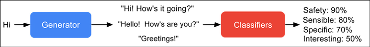
  Figure 6.10: LaMDA generates and then scores a response candidate. Source: https://ai.googleblog.com/2022/01/lamda-towards-safe-grounded-and-high.html

LaMDA demonstrated results that were impressively close to the human brain ones. According to Google (https://ai.googleblog.com/2022/01/lamda-towards-safe-grounded-and-high.html), LaMDA significantly outperformed the pretrained model in every dimension and across all model sizes. Quality metrics (Sensibleness, Specificity, and Interestingness) generally improved with the number of model parameters, with or without fine-tuning. Safety did not seem to benefit from model scaling alone, but it did improve with fine-tuning. Groundedness improved as model size increased, perhaps because larger models have a greater capacity to memorize uncommon knowledge, but fine-tuning allows the model to access external knowledge sources and to effectively shift some of the load of remembering knowledge to an external knowledge source. With fine-tuning, the quality gap to human levels can be shrunk, though the model performance remains below human levels in safety and groundedness:

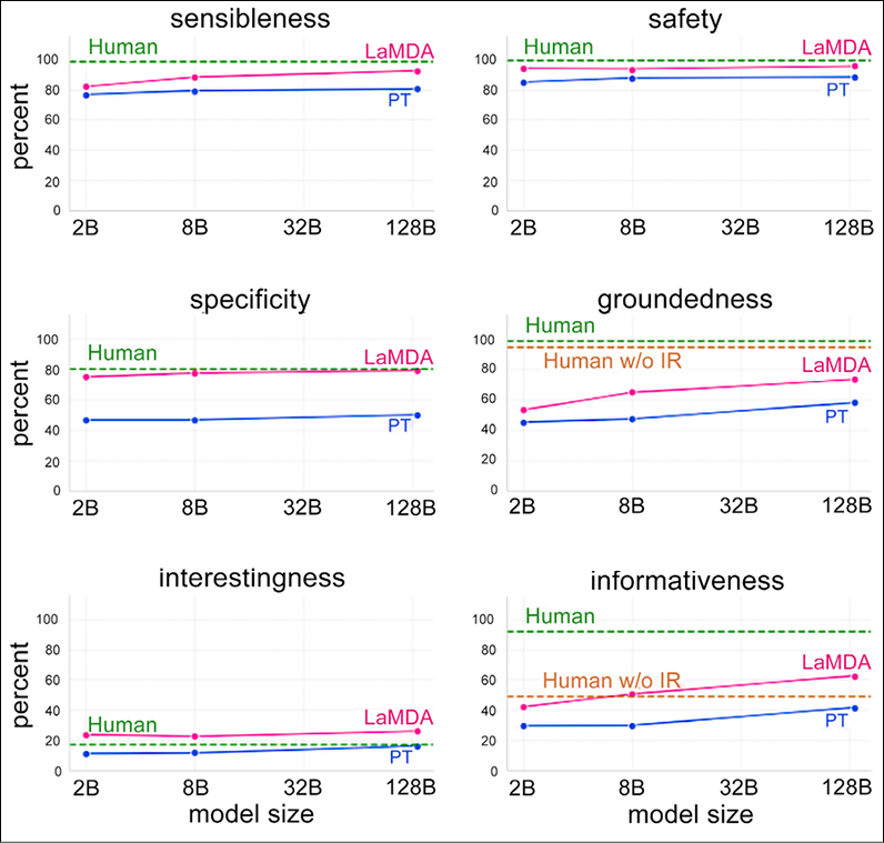
Figure 6.11: LaMDA performance – source: https://ai.googleblog.com/2022/01/lamda-towards-safe-grounded-and-high.html

Switch Transformer

The Switch Transformer is a model introduced in 2021 by Google’s researchers in Switch Transformers: Scaling to Trillion Parameter Models with Simple and Efficient Sparsity by William Fedus, Barret Zoph, and Noam Shazeer, introduced in https://arxiv.org/abs/2101.03961.

Let’s look at the key intuitions:

• The Switch Transformer was trained from 7 billion to 1.6 trillion parameters. As discussed, a typical transformer is a deep stack of multi-headed self-attention layers, and at the end of each layer, there’s an FFN aggregating the outputs coming from its multiple heads. The Switch Transformer replaces this single FFN with multiple FFNs and calls them “experts.” On each forward pass, at each layer, for each token at the input, the model activates exactly one expert:

  

  Fig 6.12: The Switch Transformer with multiple routing FFN – The dense FFN layer present in the transformer is replaced with a sparse Switch FFN layer (light blue). Source: https://arxiv.org/pdf/2101.03961.pdf

• Switch-Base (7 billion parameters) and Switch-Large (26 billion parameters) outperformed T5-Base (0.2 billion parameters) and T5-Large (0.7 billion parameters) on tasks such as language modeling, classification, coreference resolution, question answering, and summarization.

An example implementation of Switch Transformer is available at https://keras.io/examples/nlp/text_classification_with_switch_transformer/.

RETRO

RETRO (Retrieval-Enhanced Transformer) is a retrieval-enhanced autoregressive language model introduced by DeepMind in 2022 in Improving language models by retrieving from trillions of tokens by Sebastian Borgeaud et al., https://arxiv.org/pdf/2112.04426/. Let’s look at the key intuitions:

• Scaling the number of parameters in an LLM has proven to be a way to improve the quality of the results. However, this approach is not sustainable because it is computationally expensive.
• RETRO couples a retrieval Database (DB) with a transformer in a hybrid architecture. The idea is first to search with the Nearest Neighbors algorithm on pre-computed BERT embeddings stored in a retrieval DB. Then, these embeddings are used as input to a transformer’s encoder.
• The combination of retrieval and transformers allows RETRO (scaled from 150 million to 7 billion non-embedding parameters) to save on the number of parameters used by the LLM.

For instance, consider the sample query “The 2021 Women’s US Open was won” and Figure 6.13, where the cached BERT embeddings are passed to a transformer encoder to get the final result:

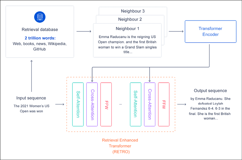
Figure 6.13: A high-level overview of Retrieval Enhanced Transformers (RETRO). Source: https://deepmind.com/research/publications/2021/improving-language-models-by-retrieving-from-trillions-of-tokens

Pathways and PaLM

Google Research announced Pathways (https://blog.google/technology/ai/introducing-pathways-next-generation-ai-architecture/), a single model that could generalize across domains and tasks while being highly efficient. Then, Google introduced Pathways Language Model (PaLM), a 540-billion parameter, dense decoder-only transformer model, which enabled us to efficiently train a single model across multiple TPU v4 Pods. Google evaluated PaLM on hundreds of language understanding and generation tasks and found that it achieves state-of-the-art performance across most tasks, by significant margins in many cases (see https://ai.googleblog.com/2022/04/pathways-language-model-palm-scaling-to.html?m=1).

Implementation

In this section, we will go through a few tasks using transformers.

Transformer reference implementation: An example of translation

In this section, we will briefly review a transformer reference implementation available at https://www.tensorflow.org/text/tutorials/transformer and specifically, we will use the opportunity to run the code in a Google Colab.

Not everyone realizes the number of GPUs it takes to train a transformer. Luckily, you can play with resources available for free at https://colab.research.google.com/github/tensorflow/text/blob/master/docs/tutorials/transformer.ipynb.

Note that implementing transformers from scratch is probably not the best choice unless you need to realize some very specific customization or you are interested in core research. If you are not interested in learning the internals, then you can skip to the next section. Our tutorial is licensed under the Creative Commons Attribution 4.0 License, and code samples are licensed under the Apache 2.0 License. The specific task we are going to perform is translating from Portuguese to English. Let’s have a look at the code, step by step:

1. First, let’s install datasets and import the right libraries. Note that the Colab available online is apparently missing the line import tensorflow_text, which is, however, added here:

   !pip install tensorflow_datasets
   !pip install -U 'tensorflow-text==2.8.*'
   import logging
   import time
   import numpy as np
   import matplotlib.pyplot as plt
   import tensorflow_text
   import tensorflow_datasets as tfds
   import tensorflow as tf
   logging.getLogger('tensorflow').setLevel(logging.ERROR)  # suppress warnings
   
2. Then, load the Portuguese to English dataset:

   examples, metadata = tfds.load('ted_hrlr_translate/pt_to_en', with_info=True,
                                  as_supervised=True)
   train_examples, val_examples = examples['train'], examples['validation']
   
3. Now, let’s convert text to sequences of token IDs, which are used as indices into an embedding:

   model_name = 'ted_hrlr_translate_pt_en_converter'
   tf.keras.utils.get_file(
       f'{model_name}.zip',
       f'https://storage.googleapis.com/download.tensorflow.org/models/{model_name}.zip',
       cache_dir='.', cache_subdir='', extract=True
   )
   tokenizers = tf.saved_model.load(model_name)
   
4. Let’s see the tokenized IDs and tokenized words:

   for pt_examples, en_examples in train_examples.batch(3).take(1):
     print('> Examples in Portuguese:')
   for en in en_examples.numpy():
     print(en.decode('utf-8'))
   

   and when you improve searchability , you actually take away the one advantage of print , which is serendipity .
   but what if it were active ?
   but they did n't test for curiosity .
   

   encoded = tokenizers.en.tokenize(en_examples)
   for row in encoded.to_list():
     print(row)
   

   [2, 72, 117, 79, 1259, 1491, 2362, 13, 79, 150, 184, 311, 71, 103, 2308, 74, 2679, 13, 148, 80, 55, 4840, 1434, 2423, 540, 15, 3]
   [2, 87, 90, 107, 76, 129, 1852, 30, 3]
   [2, 87, 83, 149, 50, 9, 56, 664, 85, 2512, 15, 3]
   

   round_trip = tokenizers.en.detokenize(encoded)
   for line in round_trip.numpy():
     print(line.decode('utf-8'))
   

   and when you improve searchability , you actually take away the one advantage of print , which is serendipity .
   but what if it were active ?
   but they did n ' t test for curiosity .
   

5. Now let’s create an input pipeline. First, we define a function to drop the examples longer than MAX_TOKENS. Second, we define a function that tokenizes the batches of raw text. Third, we create the batches:

   MAX_TOKENS=128
   def filter_max_tokens(pt, en):
     num_tokens = tf.maximum(tf.shape(pt)[1],tf.shape(en)[1])
     return num_tokens < MAX_TOKENS
   def tokenize_pairs(pt, en):
       pt = tokenizers.pt.tokenize(pt)
       # Convert from ragged to dense, padding with zeros.
       pt = pt.to_tensor()
       en = tokenizers.en.tokenize(en)
       # Convert from ragged to dense, padding with zeros.
       en = en.to_tensor()
       return pt, en
   BUFFER_SIZE = 20000
   BATCH_SIZE = 64
   def make_batches(ds):
     return (
         ds
         .cache()
         .shuffle(BUFFER_SIZE)
         .batch(BATCH_SIZE)
         .map(tokenize_pairs, num_parallel_calls=tf.data.AUTOTUNE)
         .filter(filter_max_tokens)
         .prefetch(tf.data.AUTOTUNE))
   train_batches = make_batches(train_examples)
   val_batches = make_batches(val_examples)
   
6. Now we add positional encoding, forcing tokens to be closer to each other based on the similarity of their meaning and their position in the sentence, in the d-dimensional embedding space:

   def get_angles(pos, i, d_model):
     angle_rates = 1 / np.power(10000, (2 * (i//2)) / np.float32(d_model))
     return pos * angle_rates
   def positional_encoding(position, d_model):
     angle_rads = get_angles(np.arange(position)[:, np.newaxis],
                             np.arange(d_model)[np.newaxis, :],
                             d_model)
     # apply sin to even indices in the array; 2i
     angle_rads[:, 0::2] = np.sin(angle_rads[:, 0::2])
     # apply cos to odd indices in the array; 2i+1
     angle_rads[:, 1::2] = np.cos(angle_rads[:, 1::2])
     pos_encoding = angle_rads[np.newaxis, ...]
     return tf.cast(pos_encoding, dtype=tf.float32)
   
7. Let’s now focus on the masking process. The look-ahead mask is used to mask the future tokens in a sequence, with the mask indicating which entries should not be used. For instance, to predict the third token, only the first and second tokens will be used, and to predict the fourth token, only the first, second, and third tokens will be used, and so on:

   def create_padding_mask(seq):
     seq = tf.cast(tf.math.equal(seq, 0), tf.float32)
     # add extra dimensions to add the padding
     # to the attention logits.
     return seq[:, tf.newaxis, tf.newaxis, :]  # (batch_size, 1, 1, seq_len)
   def create_look_ahead_mask(size):
     mask = 1 - tf.linalg.band_part(tf.ones((size, size)), -1, 0)
     return mask  # (seq_len, seq_len)
   
8. We are getting closer and closer to the essence of transformers. Let’s define the attention function as a scaled dot-product:

   def scaled_dot_product_attention(q, k, v, mask):
     """Calculate the attention weights.
     q, k, v must have matching leading dimensions.
     k, v must have matching penultimate dimension, i.e.: seq_len_k = seq_len_v.
     The mask has different shapes depending on its type(padding or look ahead)
     but it must be broadcastable for addition.
     Args:
       q: query shape == (..., seq_len_q, depth)
       k: key shape == (..., seq_len_k, depth)
       v: value shape == (..., seq_len_v, depth_v)
       mask: Float tensor with shape broadcastable
             to (..., seq_len_q, seq_len_k). Defaults to None.
     Returns:
       output, attention_weights
     """
     matmul_qk = tf.matmul(q, k, transpose_b=True)  # (..., seq_len_q, seq_len_k)
     # scale matmul_qk
     dk = tf.cast(tf.shape(k)[-1], tf.float32)
     scaled_attention_logits = matmul_qk / tf.math.sqrt(dk)
     # add the mask to the scaled tensor.
     if mask is not None:
       scaled_attention_logits += (mask * -1e9)
     # softmax is normalized on the last axis (seq_len_k) so that the scores
     # add up to 1.
     attention_weights = tf.nn.softmax(scaled_attention_logits, axis=-1)  # (..., seq_len_q, seq_len_k)
     output = tf.matmul(attention_weights, v)  # (..., seq_len_q, depth_v)
     return output, attention_weights
   
9. Now that the attention is defined, we need to implement the multi-head mechanism. There are three parts: linear layers, scaled dot-product attention, and the final linear layer (see Figure 6.14):

   

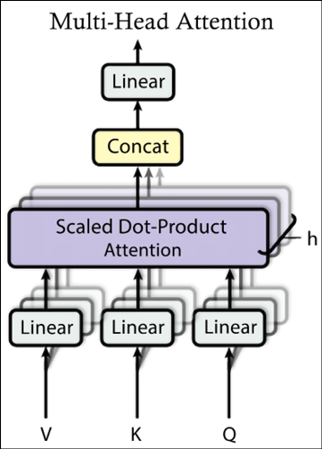
   Figure 6.14: Multi-head attention

   class MultiHeadAttention(tf.keras.layers.Layer):
     def __init__(self,*, d_model, num_heads):
       super(MultiHeadAttention, self).__init__()
       self.num_heads = num_heads
       self.d_model = d_model
       assert d_model % self.num_heads == 0
       self.depth = d_model // self.num_heads
       self.wq = tf.keras.layers.Dense(d_model)
       self.wk = tf.keras.layers.Dense(d_model)
       self.wv = tf.keras.layers.Dense(d_model)
       self.dense = tf.keras.layers.Dense(d_model)
     def split_heads(self, x, batch_size):
       """Split the last dimension into (num_heads, depth).
       Transpose the result such that the shape is (batch_size, num_heads, seq_len, depth)
       """
       x = tf.reshape(x, (batch_size, -1, self.num_heads, self.depth))
       return tf.transpose(x, perm=[0, 2, 1, 3])
     def call(self, v, k, q, mask):
       batch_size = tf.shape(q)[0]
       q = self.wq(q)  # (batch_size, seq_len, d_model)
       k = self.wk(k)  # (batch_size, seq_len, d_model)
       v = self.wv(v)  # (batch_size, seq_len, d_model)
       q = self.split_heads(q, batch_size)  # (batch_size, num_heads, seq_len_q, depth)
       k = self.split_heads(k, batch_size)  # (batch_size, num_heads, seq_len_k, depth)
       v = self.split_heads(v, batch_size)  # (batch_size, num_heads, seq_len_v, depth)
       # scaled_attention.shape == (batch_size, num_heads, seq_len_q, depth)
       # attention_weights.shape == (batch_size, num_heads, seq_len_q, seq_len_k)
       scaled_attention, attention_weights = scaled_dot_product_attention(
           q, k, v, mask)
       scaled_attention = tf.transpose(scaled_attention, perm=[0, 2, 1, 3])  # (batch_size, seq_len_q, num_heads, depth)
       concat_attention = tf.reshape(scaled_attention,
                                     (batch_size, -1, self.d_model))  # (batch_size, seq_len_q, d_model)
       output = self.dense(concat_attention)  # (batch_size, seq_len_q, d_model)
       return output, attention_weights
   

10. Now, we can define a point-wise feedforward network that consists of two fully connected layers with a ReLU activation in between:

    def point_wise_feed_forward_network(d_model, dff):
     return tf.keras.Sequential([
         tf.keras.layers.Dense(dff, activation='relu'),  # (batch_size, seq_len, dff)
         tf.keras.layers.Dense(d_model)  # (batch_size, seq_len, d_model)
     ])
    
11. We can now concentrate on defining the encoder and decoder parts as described in Figure 6.15. Remember that the traditional transformer takes the input sentence through N encoder layers, while the decoder uses the encoder output and its own input (self-attention) to predict the next word. Each encoder layer has sublayers made by multi-head attention (with a padding mask) and then point-wise feedforward networks. Each sublayer uses a residual connection to contain the problem of vanishing gradient, and a normalization layer:

    class EncoderLayer(tf.keras.layers.Layer):
      def __init__(self,*, d_model, num_heads, dff, rate=0.1):
        super(EncoderLayer, self).__init__()
        self.mha = MultiHeadAttention(d_model=d_model, num_heads=num_heads)
        self.ffn = point_wise_feed_forward_network(d_model, dff)
        self.layernorm1 = tf.keras.layers.LayerNormalization(epsilon=1e-6)
        self.layernorm2 = tf.keras.layers.LayerNormalization(epsilon=1e-6)
        self.dropout1 = tf.keras.layers.Dropout(rate)
        self.dropout2 = tf.keras.layers.Dropout(rate)
      def call(self, x, training, mask):
        attn_output, _ = self.mha(x, x, x, mask)  # (batch_size, input_seq_len, d_model)
        attn_output = self.dropout1(attn_output, training=training)
        out1 = self.layernorm1(x + attn_output)  # (batch_size, input_seq_len, d_model)
        ffn_output = self.ffn(out1)  # (batch_size, input_seq_len, d_model)
        ffn_output = self.dropout2(ffn_output, training=training)
        out2 = self.layernorm2(out1 + ffn_output)  # (batch_size, input_seq_len, d_model)
        return out2
    
12. Each decoder layer is made of sublayers. First, a masked multi-head attention (with a look-ahead mask and padding mask). Then, a multi-head attention (with a padding mask), V (value), and K (key) receive the encoder output as inputs. Q (query) receives the output from the masked multi-head attention sublayer and, finally, the point-wise feedforward networks:

    class DecoderLayer(tf.keras.layers.Layer):
      def __init__(self,*, d_model, num_heads, dff, rate=0.1):
        super(DecoderLayer, self).__init__()
        self.mha1 = MultiHeadAttention(d_model=d_model, num_heads=num_heads)
        self.mha2 = MultiHeadAttention(d_model=d_model, num_heads=num_heads)
        self.ffn = point_wise_feed_forward_network(d_model, dff)
        self.layernorm1 = tf.keras.layers.LayerNormalization(epsilon=1e-6)
        self.layernorm2 = tf.keras.layers.LayerNormalization(epsilon=1e-6)
        self.layernorm3 = tf.keras.layers.LayerNormalization(epsilon=1e-6)
        self.dropout1 = tf.keras.layers.Dropout(rate)
        self.dropout2 = tf.keras.layers.Dropout(rate)
        self.dropout3 = tf.keras.layers.Dropout(rate)
      def call(self, x, enc_output, training,
               look_ahead_mask, padding_mask):
        # enc_output.shape == (batch_size, input_seq_len, d_model)
        attn1, attn_weights_block1 = self.mha1(x, x, x, look_ahead_mask)  # (batch_size, target_seq_len, d_model)
        attn1 = self.dropout1(attn1, training=training)
        out1 = self.layernorm1(attn1 + x)
        attn2, attn_weights_block2 = self.mha2(
            enc_output, enc_output, out1, padding_mask)  # (batch_size, target_seq_len, d_model)
        attn2 = self.dropout2(attn2, training=training)
        out2 = self.layernorm2(attn2 + out1)  # (batch_size, target_seq_len, d_model)
        ffn_output = self.ffn(out2)  # (batch_size, target_seq_len, d_model)
        ffn_output = self.dropout3(ffn_output, training=training)
        out3 = self.layernorm3(ffn_output + out2)  # (batch_size, target_seq_len, d_model)
        return out3, attn_weights_block1, attn_weights_block2
    
13. Now that we have defined the encoder layer, we can use it to define the proper encoder. This consists of three stages: input embedding, positional encoding, and N encoder layers:

    class Encoder(tf.keras.layers.Layer):
      def __init__(self,*, num_layers, d_model, num_heads, dff, input_vocab_size,
                   rate=0.1):
        super(Encoder, self).__init__()
        self.d_model = d_model
        self.num_layers = num_layers
        self.embedding = tf.keras.layers.Embedding(input_vocab_size, d_model)
        self.pos_encoding = positional_encoding(MAX_TOKENS, self.d_model)
        self.enc_layers = [
            EncoderLayer(d_model=d_model, num_heads=num_heads, dff=dff, rate=rate)
            for _ in range(num_layers)]
        self.dropout = tf.keras.layers.Dropout(rate)
      def call(self, x, training, mask):
        seq_len = tf.shape(x)[1]
        # adding embedding and position encoding.
        x = self.embedding(x)  # (batch_size, input_seq_len, d_model)
        x *= tf.math.sqrt(tf.cast(self.d_model, tf.float32))
        x += self.pos_encoding[:, :seq_len, :]
        x = self.dropout(x, training=training)
        for i in range(self.num_layers):
          x = self.enc_layers[i](x, training, mask)
        return x  # (batch_size, input_seq_len, d_model)
    
14. We can now focus our attention on the decoder itself. It consists of output embedding, positional encoding, and N decoder layers:

    class Decoder(tf.keras.layers.Layer):
      def __init__(self,*, num_layers, d_model, num_heads, dff, target_vocab_size,
                   rate=0.1):
        super(Decoder, self).__init__()
        self.d_model = d_model
        self.num_layers = num_layers
        self.embedding = tf.keras.layers.Embedding(target_vocab_size, d_model)
        self.pos_encoding = positional_encoding(MAX_TOKENS, d_model)
        self.dec_layers = [
            DecoderLayer(d_model=d_model, num_heads=num_heads, dff=dff, rate=rate)
            for _ in range(num_layers)]
        self.dropout = tf.keras.layers.Dropout(rate)
      def call(self, x, enc_output, training,
               look_ahead_mask, padding_mask):
        seq_len = tf.shape(x)[1]
        attention_weights = {}
        x = self.embedding(x)  # (batch_size, target_seq_len, d_model)
        x *= tf.math.sqrt(tf.cast(self.d_model, tf.float32))
        x += self.pos_encoding[:, :seq_len, :]
        x = self.dropout(x, training=training)
        for i in range(self.num_layers):
          x, block1, block2 = self.dec_layers[i](x, enc_output, training,
                                                 look_ahead_mask, padding_mask)
          attention_weights[f'decoder_layer{i+1}_block1'] = block1
          attention_weights[f'decoder_layer{i+1}_block2'] = block2
        # x.shape == (batch_size, target_seq_len, d_model)
        return x, attention_weights
    
15. Now that we have defined the encoder and decoder, we can now turn our attention to the transformer itself, which is composed of an encoder, a decoder, and a final linear layer (see Figure 6.15):

    class Transformer(tf.keras.Model):
      def __init__(self,*, num_layers, d_model, num_heads, dff, input_vocab_size,
                   target_vocab_size, rate=0.1):
        super().__init__()
        self.encoder = Encoder(num_layers=num_layers, d_model=d_model,
                               num_heads=num_heads, dff=dff,
                               input_vocab_size=input_vocab_size, rate=rate)
        self.decoder = Decoder(num_layers=num_layers, d_model=d_model,
                               num_heads=num_heads, dff=dff,
                               target_vocab_size=target_vocab_size, rate=rate)
        self.final_layer = tf.keras.layers.Dense(target_vocab_size)
      def call(self, inputs, training):
        # Keras models prefer if you pass all your inputs in the first argument
        inp, tar = inputs
        enc_padding_mask, look_ahead_mask, dec_padding_mask = self.create_masks(inp, tar)
        enc_output = self.encoder(inp, training, enc_padding_mask)  # (batch_size, inp_seq_len, d_model)
        # dec_output.shape == (batch_size, tar_seq_len, d_model)
        dec_output, attention_weights = self.decoder(
            tar, enc_output, training, look_ahead_mask, dec_padding_mask)
        final_output = self.final_layer(dec_output)  # (batch_size, tar_seq_len, target_vocab_size)
        return final_output, attention_weights
      def create_masks(self, inp, tar):
        # Encoder padding mask
        enc_padding_mask = create_padding_mask(inp)
        # Used in the 2nd attention block in the decoder.
        # This padding mask is used to mask the encoder outputs.
        dec_padding_mask = create_padding_mask(inp)
        # Used in the 1st attention block in the decoder.
        # It is used to pad and mask future tokens in the input received by
        # the decoder.
        look_ahead_mask = create_look_ahead_mask(tf.shape(tar)[1])
        dec_target_padding_mask = create_padding_mask(tar)
        look_ahead_mask = tf.maximum(dec_target_padding_mask, look_ahead_mask)
        return enc_padding_mask, look_ahead_mask, dec_padding_mask
    

Figure 6.15: The traditional transformer

16. We are almost done. We just need to define hyperparameters and the optimizer, using exactly the same settings as the seminal paper, and the loss function:

    num_layers = 4
    d_model = 128
    dff = 512
    num_heads = 8
    dropout_rate = 0.1
    class CustomSchedule(tf.keras.optimizers.schedules.LearningRateSchedule):
      def __init__(self, d_model, warmup_steps=4000):
        super(CustomSchedule, self).__init__()
        self.d_model = d_model
        self.d_model = tf.cast(self.d_model, tf.float32)
        self.warmup_steps = warmup_steps
      def __call__(self, step):
        arg1 = tf.math.rsqrt(step)
        arg2 = step * (self.warmup_steps ** -1.5)
        return tf.math.rsqrt(self.d_model) * tf.math.minimum(arg1, arg2)
    learning_rate = CustomSchedule(d_model)
    optimizer = tf.keras.optimizers.Adam(learning_rate, beta_1=0.9, beta_2=0.98,
                                         epsilon=1e-9)
    def loss_function(real, pred):
      mask = tf.math.logical_not(tf.math.equal(real, 0))
      loss_ = loss_object(real, pred)
      mask = tf.cast(mask, dtype=loss_.dtype)
      loss_ *= mask
      return tf.reduce_sum(loss_)/tf.reduce_sum(mask)
    def accuracy_function(real, pred):
      accuracies = tf.equal(real, tf.argmax(pred, axis=2))
      mask = tf.math.logical_not(tf.math.equal(real, 0))
      accuracies = tf.math.logical_and(mask, accuracies)
      accuracies = tf.cast(accuracies, dtype=tf.float32)
      mask = tf.cast(mask, dtype=tf.float32)
      return tf.reduce_sum(accuracies)/tf.reduce_sum(mask)
    train_loss = tf.keras.metrics.Mean(name='train_loss')
    train_accuracy = tf.keras.metrics.Mean(name='train_accuracy')
    
17. Time to define the transformer. Let’s see the code:

    transformer = Transformer(
        num_layers=num_layers,
        d_model=d_model,
        num_heads=num_heads,
        dff=dff,
        input_vocab_size=tokenizers.pt.get_vocab_size().numpy(),
        target_vocab_size=tokenizers.en.get_vocab_size().numpy(),
        rate=dropout_rate)
    
18. Let’s also define the checkpoints with the following code:

    checkpoint_path = './checkpoints/train'
    ckpt = tf.train.Checkpoint(transformer=transformer,
                               optimizer=optimizer)
    ckpt_manager = tf.train.CheckpointManager(ckpt, checkpoint_path, max_to_keep=5)
    # if a checkpoint exists, restore the latest checkpoint.
    if ckpt_manager.latest_checkpoint:
      ckpt.restore(ckpt_manager.latest_checkpoint)
      print('Latest checkpoint restored!!')
    
19. Remember that the transformer is autoregressive. The current output is used to predict what will happen next. We use a look-ahead mask, to prevent the model from peeking at the expected output. We are now ready to define train_step:

    train_step_signature = [
        tf.TensorSpec(shape=(None, None), dtype=tf.int64),
        tf.TensorSpec(shape=(None, None), dtype=tf.int64),
    ]
    @tf.function(input_signature=train_step_signature)
    def train_step(inp, tar):
      tar_inp = tar[:, :-1]
      tar_real = tar[:, 1:]
      with tf.GradientTape() as tape:
        predictions, _ = transformer([inp, tar_inp],
                                     training = True)
        loss = loss_function(tar_real, predictions)
      gradients = tape.gradient(loss, transformer.trainable_variables)
      optimizer.apply_gradients(zip(gradients, transformer.trainable_variables))
      train_loss(loss)
      train_accuracy(accuracy_function(tar_real, predictions))
    EPOCHS = 20
    for epoch in range(EPOCHS):
      start = time.time()
      train_loss.reset_states()
      train_accuracy.reset_states()
      # inp -> portuguese, tar -> english
      for (batch, (inp, tar)) in enumerate(train_batches):
        train_step(inp, tar)
        if batch % 50 == 0:
          print(f'Epoch {epoch + 1} Batch {batch} Loss {train_loss.result():.4f} Accuracy {train_accuracy.result():.4f}')
      if (epoch + 1) % 5 == 0:
        ckpt_save_path = ckpt_manager.save()
        print(f'Saving checkpoint for epoch {epoch+1} at {ckpt_save_path}')
      print(f'Epoch {epoch + 1} Loss {train_loss.result():.4f} Accuracy {train_accuracy.result():.4f}')
      print(f'Time taken for 1 epoch: {time.time() - start:.2f} secs
    ')
    

    After running the training step in Colab, we get the following situation:

    Epoch 20 Loss 1.5030 Accuracy 0.6720
    Time taken for 1 epoch: 169.01 secs
    

20. We are now ready for translation. The following steps are used to translate:
    1. Encode the input sentence using the Portuguese tokenizer (tokenizers.pt).
    2. The decoder input is initialized to the [START] token.
    3. Calculate the padding masks and the look-ahead masks.
    4. The decoder then outputs the predictions by looking at the encoder output and its own output (self-attention).
    5. Concatenate the predicted token to the decoder input and pass it to the decoder:

    class Translator(tf.Module):
      def __init__(self, tokenizers, transformer):
        self.tokenizers = tokenizers
        self.transformer = transformer
      def __call__(self, sentence, max_length=MAX_TOKENS):
        # input sentence is portuguese, hence adding the start and end token
        assert isinstance(sentence, tf.Tensor)
        if len(sentence.shape) == 0:
          sentence = sentence[tf.newaxis]
        sentence = self.tokenizers.pt.tokenize(sentence).to_tensor()
        encoder_input = sentence
        # As the output language is english, initialize the output with the
        # english start token.
        start_end = self.tokenizers.en.tokenize([''])[0]
        start = start_end[0][tf.newaxis]
        end = start_end[1][tf.newaxis]
        # 'tf.TensorArray' is required here (instead of a python list) so that the
        # dynamic-loop can be traced by 'tf.function'.
        output_array = tf.TensorArray(dtype=tf.int64, size=0, dynamic_size=True)
        output_array = output_array.write(0, start)
        for i in tf.range(max_length):
          output = tf.transpose(output_array.stack())
          predictions, _ = self.transformer([encoder_input, output], training=False)
          # select the last token from the seq_len dimension
          predictions = predictions[:, -1:, :]  # (batch_size, 1, vocab_size)
          predicted_id = tf.argmax(predictions, axis=-1)
          # concatentate the predicted_id to the output which is given to the decoder
          # as its input.
          output_array = output_array.write(i+1, predicted_id[0])
          if predicted_id == end:
            break
        output = tf.transpose(output_array.stack())
        # output.shape (1, tokens)
        text = tokenizers.en.detokenize(output)[0]  # shape: ()
        tokens = tokenizers.en.lookup(output)[0]
        # 'tf.function' prevents us from using the attention_weights that were
        # calculated on the last iteration of the loop. So recalculate them outside
        # the loop.
        _, attention_weights = self.transformer([encoder_input, output[:,:-1]], training=False)
        return text, tokens, attention_weights
    
21. Let’s call the translator on a sample sentence with this code snippet:

    translator = Translator(tokenizers, transformer)
    def print_translation(sentence, tokens, ground_truth):
      print(f'{"Input:":15s}: {sentence}')
      print(f'{"Prediction":15s}: {tokens.numpy().decode("utf-8")}')
      print(f'{"Ground truth":15s}: {ground_truth}')
    sentence = 'os meus vizinhos ouviram sobre esta ideia.'
    ground_truth = 'and my neighboring homes heard about this idea .'
    translated_text, translated_tokens, attention_weights = translator(
        tf.constant(sentence))
    print_translation(sentence, translated_text, ground_truth)
    

    Getting as the result:

    Input:         : os meus vizinhos ouviram sobre esta ideia.
    Prediction     : my neighbors have heard about this idea .
    Ground truth   : and my neighboring homes heard about this idea .
    

In this detailed analysis, we have discussed how a traditional transformer is implemented taking positional encoding, multi-head attention, and masking into account. The analyzed code is at https://www.tensorflow.org/text/tutorials/transformer.

Next, we will discuss how to use transformers making use of higher-level libraries.

Hugging Face

As discussed, implementing transformers from scratch is probably not the best choice unless you need to realize some very specific customization, or you are interested in core research. This is useful if you want to understand the internal details of a transformer architecture, or perhaps modify the transformer architecture to produce a new variant. Nowadays, there are very good libraries providing high-quality solutions. One of them is Hugging Face, which provides some efficient tools. Hugging Face is built around the idea of commercializing its open source transformers library. Let’s see why the library became so popular:

• Hugging Face provides a common API to handle many transformer architectures.
• It not only provides the base model, but models with different types of “head” to handle specific tasks (for example, for the BERT architecture it provides TFBertModel, and the TFBertForSequenceClassification for tasks like sentiment analysis, TFBertForTokenClassification for tasks like named entity recognition, and TFBertForQuestionAnswering for Q and A, among others).
• You can also create your own network for a specific task quite easily by using the pretrained weights provided here, for example, by using TFBertForPreTraining.
• In addition to the pipeline() method in the next subsection, we can also define a model in the regular way and use fit() to train it and predict() to make inferences against it, just like a normal TF model (PyTorch also has the Trainer interface). We will see an example later on in this chapter.

Now, let’s check some examples of how to use Hugging Face.

Generating text

In this section, we are going to use GPT-2 for natural language generation, a software process for producing natural language outputs. Let’s start from the beginning by installing the Hugging Face library:

1. The first step is to create a dedicated virtual environment, where we can install the transformer library. In my case, I use the library for TensorFlow 2.0:

   python -m venv .env
   source .env/bin/activate
   pip install transformers[tf-cpu]
   
2. Then let’s verify that everything is working correctly by downloading a pretrained model used for sentiment analysis:

   python -c "from transformers import pipeline; print(pipeline('sentiment-analysis')('we love you'))"
   

   Since the expected sentiment should be very positive, we shall see something like the following:

   [{'label': 'POSITIVE', 'score': 0.9998704791069031}]
   

3. Now let’s focus on generating text with GPT-2:

   from transformers import pipeline
   generator = pipeline(task="text-generation")
   

   You should see something like the following:

   No model was supplied, defaulted to gpt2 (https://huggingface.co/gpt2)
   Downloading: 100%|██████████████████████████████| 665/665 [00:00<00:00, 167kB/s]
   Downloading: 100%|███████████████████████████| 475M/475M [03:24<00:00, 2.44MB/s
   

4. Let’s pass some text to the generator and see what the result is. The first sentence is extracted from Tolkien’s work, the second from Einstein’s theories, and the third one comes from “Harry Potter”:

   generator("Three Rings for the Elven-kings under the sky, Seven for the Dwarf-lords in their halls of stone")
   

   Setting 'pad_token_id' to 50256 (first 'eos_token_id') to generate sequence
   [{'generated_text': 'Three Rings for the Elven-kings under the sky, Seven for the Dwarf-lords in their halls of stone and Eight for the Dwarves in their halls of rock! Three new Rings of the Elven-kings under the sky, Seven for'}]
   

   generator ("The original theory of relativity is based upon the premise that all coordinate systems in relative uniform translatory motion to each other are equally valid and equivalent ")
   

   Setting 'pad_token_id' to 50256 (first 'eos_token_id') to generate sequence
   [{'generated_text': 'The original theory of relativity is based upon the premise that all coordinate systems in relative uniform translatory motion to each other are equally valid and equivalent xa0to one another. In other words, they can all converge, and therefore all the laws are valid'}]
   

   generator ("It takes a great deal of bravery to stand up to our enemies")
   

   Setting 'pad_token_id' to 50256 (first 'eos_token_id') to generate sequence
   [{'generated_text': 'It takes a great deal of bravery to stand up to our enemies that day. She still has a lot to learn from it, or it could take decades to do.
   
   While some braver men struggle, many are not as lucky'}]
   

Pretty easy, isn’t it?

Autoselecting a model and autotokenization

Hugging Face does a great job of helping the developer to automate as many steps as possible. Let’s see some examples:

1. You can easily import a pretrained model among the several dozen available. A complete list of available models is here: https://huggingface.co/docs/transformers/model_doc/auto:

   from transformers import TFAutoModelForSequenceClassification
   model = TFAutoModelForSequenceClassification.from_pretrained("distilbert-base-uncased")
   

   Downloading: 100%|█████████████████████████████| 483/483 [00:00<00:00, 68.9kB/s]
   Downloading: 100%|███████████████████████████| 347M/347M [01:05<00:00, 5.59MB/s]
   …
   

   You should probably train this model on a downstream task to use it for predictions and inference.

2. You can use AutoTokenizer to transform words into tokens used by the models:

   from transformers import AutoTokenizer
   tokenizer = AutoTokenizer.from_pretrained("bert-base-uncased")
   sequence = "The original theory of relativity is based upon the premise that all coordinate systems"
   print(tokenizer(sequence))
   

   {'input_ids': [101, 1996, 2434, 3399, 1997, 20805, 2003, 2241, 2588, 1996, 18458, 2008, 2035, 13530, 3001, 102], 'token_type_ids': [0, 0, 0, 0, 0, 0, 0, 0, 0, 0, 0, 0, 0, 0, 0, 0], 'attention_mask': [1, 1, 1, 1, 1, 1, 1, 1, 1, 1, 1, 1, 1, 1, 1, 1]}
   

Named entity recognition

Named Entity Recognition (NER) is a classical NLP task. According to Wikipedia, named entity recognition – also known as (named) entity identification, entity chunking, and entity extraction – is a subtask of information extraction that seeks to locate and classify named entities mentioned in unstructured text into predefined categories such as person names, organizations, locations, medical codes, time expressions, quantities, monetary values, and percentages, among others.

Let’s see how easily this task can be performed with Hugging Face:

1. First of all, let’s create a NER pipeline:

   from transformers import pipeline
   ner_pipe = pipeline("ner")
   sequence = """Mr. and Mrs. Dursley, of number four, Privet Drive, were proud to say that they were perfectly normal, thank you very much."""
   for entity in ner_pipe(sequence):
       print(entity) 
   
2. You will be able to see something like the following, where the entities are recognized:

   {'entity': 'I-PER', 'score': 0.99908304, 'index': 6, 'word': 'Du', 'start': 13, 'end': 15}
   {'entity': 'I-PER', 'score': 0.9869529, 'index': 7, 'word': '##rs', 'start': 15, 'end': 17}
   {'entity': 'I-PER', 'score': 0.9784202, 'index': 8, 'word': '##ley', 'start': 17, 'end': 20}
   {'entity': 'I-ORG', 'score': 0.6860208, 'index': 14, 'word': 'P', 'start': 38, 'end': 39}
   {'entity': 'I-ORG', 'score': 0.7713562, 'index': 15, 'word': '##rive', 'start': 39, 'end': 43}
   {'entity': 'I-ORG', 'score': 0.76567733, 'index': 16, 'word': '##t', 'start': 43, 'end': 44}
   {'entity': 'I-ORG', 'score': 0.8087192, 'index': 17, 'word': 'Drive', 'start': 45, 'end': 50}
   

Named entity recognition can understand nine different classes:

• O: Outside of a named entity.
• B-MIS: Beginning of a miscellaneous entity right after another miscellaneous entity.
• I-MIS: Miscellaneous entity.
• B-PER: Beginning of a person’s name right after another person’s name.
• I-PER: A person’s name.
• B-ORG: Beginning of an organization right after another organization.
• I-ORG: Organization.
• B-LOC: Beginning of a location right after another location.
• I-LOC: Location.

These entities are defined in the CoNLL-2003 dataset typically used for this task and automatically selected by Hugging Face.

Summarization

Let’s now turn our attention to summarization, meaning the task of expressing the most important facts or ideas about something or someone in a short and clear form. Hugging Face makes it incredibly easy to use the T5 model as default for this task. Let’s see the code:

1. First of all, let’s create a summarization pipeline using the default T5 small model:

   from transformers import pipeline
   summarizer = pipeline("summarization")
   ARTICLE = """
    Mr.
    and Mrs.
    Dursley, of number four, Privet Drive, were proud to say
    that they were perfectly normal, thank you very much.
    They were the last
    people you'd expect to be involved in anything strange or mysterious,
   because they just didn't hold with such nonsense.
    Mr.
    Dursley was the director of a firm called Grunnings, which made
    drills.
    He was a big, beefy man with hardly any neck, although he did
    have a very large mustache.
    Mrs.
    Dursley was thin and blonde and had
    nearly twice the usual amount of neck, which came in very useful as she
    spent so much of her time craning over garden fences, spying on the
    neighbors.
    The Dursleys had a small son called Dudley and in their
    opinion there was no finer boy anywhere"""
   print(summarizer(ARTICLE, max_length=130, min_length=30, do_sample=False))
   
2. As a result, we will see something similar to the following:

   No model was supplied, defaulted to t5-small (https://huggingface.co/t5-small)
   Downloading: 100%|██████████████████████████| 1.17k/1.17k [00:00<00:00, 300kB/s]
   Downloading: 100%|███████████████████████████| 231M/231M [01:29<00:00, 2.71MB/s]
   [{'summary_text': "Mr. and Mrs. Dursley, of number four, were the last people you'd expect to be involved in anything strange or mysterious . the Dursleys had a small son called Dudley and in their opinion there was no finer boy anywhere ."}]
   
3. Suppose that you want to change to a different model. That’s extremely simple as you only need to change one parameter:

   summarizer = pipeline("summarization", model='t5-base')
   
4. As a result, we can see something like the following:

   Downloading: 100%|████████████████████████████████████████████████████████████| 773k/773k [00:00<00:00, 1.28MB/s]
   Downloading: 100%|██████████████████████████████████████████████████████████| 1.32M/1.32M [00:00<00:00, 1.93MB/s]
   [{'summary_text': "bob greene says he and his wife were perfectly normal . he says they were the last people you'd expect to be involved in anything strange or mysterious . greene: they were a big, beefy man with hardly any neck, but had a very large mustache ."}]
   

Fine-tuning

One common usage pattern for transformers is to use a pretrained LLM and then fine-tune the model for specific downstream tasks. Of course, the fine-tuning steps will take place on your own dataset, while pretraining is performed on very large datasets. The advantages of this two-step strategy are in terms of both saving computation costs and in reducing the carbon footprint. Plus, fine-tuning allows you to use state-of-the-art models without having to train one from scratch. Let’s see how to fine-tune a model with TF. This example is available at https://huggingface.co/docs/transformers/training, where the pretrained model used is bert-base-cased, which is fine-tuned on the “Yelp Reviews” dataset (available at https://huggingface.co/datasets/yelp_review_full). Let’s see the code from https://huggingface.co/docs/transformers/training

1. First, let’s load and tokenize the Yelp dataset:

   from datasets import load_dataset
   dataset = load_dataset("yelp_review_full")
   from transformers import AutoTokenizer
   tokenizer = AutoTokenizer.from_pretrained("bert-base-cased")
   def tokenize_function(examples):
       return tokenizer(examples["text"], padding="max_length", truncation=True)
   tokenized_datasets = dataset.map(tokenize_function, batched=True)
   small_train_dataset = tokenized_datasets["train"].shuffle(seed=42).select(range(1000))
   small_eval_dataset = tokenized_datasets["test"].shuffle(seed=42).select(range(1000))
   
2. Then let’s convert them to TF format datasets:

   from transformers import DefaultDataCollator
   data_collator = DefaultDataCollator(return_tensors="tf")
   # convert the tokenized datasets to TensorFlow datasets
   tf_train_dataset = small_train_dataset.to_tf_dataset(
       columns=["attention_mask", "input_ids", "token_type_ids"],
       label_cols=["labels"],
       shuffle=True,
       collate_fn=data_collator,
       batch_size=8,
   )
   tf_validation_dataset = small_eval_dataset.to_tf_dataset(
       columns=["attention_mask", "input_ids", "token_type_ids"],
       label_cols=["labels"],
       shuffle=False,
       collate_fn=data_collator,
       batch_size=8,
   )
   
3. Now, we can use TFAutoModelForSequenceClassification, specifically selecting bert-base-cased:

   import tensorflow as tf
   from transformers import TFAutoModelForSequenceClassification
   model = TFAutoModelForSequenceClassification.from_pretrained("bert-base-cased", num_labels=5)
   
4. Finally, the fine-tuning is simply using the standard way to train a model used in Keras/TF 2.0 by compiling the model and then using fit on it:

   model.compile(
       optimizer=tf.keras.optimizers.Adam(learning_rate=5e-5),
       loss=tf.keras.losses.SparseCategoricalCrossentropy(from_logits=True),
       metrics=tf.metrics.SparseCategoricalAccuracy(),
   )
   model.fit(tf_train_dataset, validation_data=tf_validation_dataset, epochs=3)
   

If you want, you can test the code on a public Colab notebook (available at https://huggingface.co/docs/transformers/training). If you run the code yourself, you should be able to see something similar to Figure 6.16:

Figure 6.16: Fine-tuning BERT on a Colab notebook

Next, we are going to introduce TFHub.

TFHub

In the previous section, we discussed how to use the Hugging Face Transformer library. Now, we will have a look at another library known as TFHub available at https://tfhub.dev/. TensorFlow Hub is a repository of trained machine learning models ready for fine-tuning and deployable anywhere. The key idea is to reuse trained models like BERT and Faster R-CNN with just a few lines of code.

Using TFHub is as easy as writing a few lines of code. Let’s see a simple example where we load a pretrained model for computing embeddings. In this case, we use nnlm-en-dim128, a token-based text embedding trained on the English Google News 200B corpus:

!pip install --upgrade tensorflow_hub
import tensorflow_hub as hub
model = hub.KerasLayer("https://tfhub.dev/google/nnlm-en-dim128/2")
embeddings = model(["The rain in Spain.", "falls",
                    "mainly", "In the plain!"])
print(embeddings.shape)  #(4,128)

Now let’s see how to use BERT. This code is adapted from https://www.tensorflow.org/hub/tutorials/bert_experts, and it is also available on Hugging Face (https://huggingface.co/docs/transformers/training):

1. Let’s set up the environment and import useful modules:

   !pip install seaborn
   !pip install sklearn
   !pip install tensorflow_hub
   !pip install tensorflow_text
   import seaborn as sns
   from sklearn.metrics import pairwise
   import tensorflow as tf
   import tensorflow_hub as hub
   import tensorflow_text as text  # Imports TF ops for preprocessing.
   
2. Let’s define a few sentences used for comparing their similarities:

   sentences = [
       "Do not pity the dead, Harry. Pity the living, and, above all those who live without love.",
       "It is impossible to manufacture or imitate love",
       "Differences of habit and language are nothing at all if our aims are identical and our hearts are open.",
       "What do I care how he looks? I am good-looking enough for both of us, I theenk! All these scars show is zat my husband is brave!",
       "Love as powerful as your mother's for you leaves it's own mark. To have been loved so deeply, even though the person who loved us is gone, will give us some protection forever.",
       "Family…Whatever yeh say, blood's important. . . .",
       "I cared more for your happiness than your knowing the truth, more for your peace of mind than my plan, more for your life than the lives that might be lost if the plan failed."
   ]
   
3. Then, let’s use a pretrained BERT model available on TFHub to compute embeddings on the input sentences just defined. BERT’s output is the set of embeddings itself:

   #@title Configure the model { run: "auto" }
   BERT_MODEL = "https://tfhub.dev/google/experts/bert/wiki_books/2" # @param {type: "string"} ["https://tfhub.dev/google/experts/bert/wiki_books/2", "https://tfhub.dev/google/experts/bert/wiki_books/mnli/2", "https://tfhub.dev/google/experts/bert/wiki_books/qnli/2", "https://tfhub.dev/google/experts/bert/wiki_books/qqp/2", "https://tfhub.dev/google/experts/bert/wiki_books/squad2/2", "https://tfhub.dev/google/experts/bert/wiki_books/sst2/2",  "https://tfhub.dev/google/experts/bert/pubmed/2", "https://tfhub.dev/google/experts/bert/pubmed/squad2/2"]
   # Preprocessing must match the model, but all the above use the same.
   PREPROCESS_MODEL = "https://tfhub.dev/tensorflow/bert_en_uncased_preprocess/3"
   preprocess = hub.load(PREPROCESS_MODEL)
   bert = hub.load(BERT_MODEL)
   inputs = preprocess(sentences)
   outputs = bert(inputs)
   
4. Now let’s define some auxiliary functions to show the similarity among embeddings based on pairwise.cosine_similarity:

   def plot_similarity(features, labels):
     """Plot a similarity matrix of the embeddings."""
     cos_sim = pairwise.cosine_similarity(features)
     sns.set(font_scale=1.2)
     cbar_kws=dict(use_gridspec=False, location="left")
     g = sns.heatmap(
         cos_sim, xticklabels=labels, yticklabels=labels,
         vmin=0, vmax=1, cmap="Blues", cbar_kws=cbar_kws)
     g.tick_params(labelright=True, labelleft=False)
     g.set_yticklabels(labels, rotation=0)
     g.set_title("Semantic Textual Similarity")
   plot_similarity(outputs["pooled_output"], sentences)
   

The interested reader can access the Colab notebook online on the Hugging Face website (available at https://huggingface.co/docs/transformers/training) and visualize a heatmap showing similarities among sentences. Overall, using LLMs with TFHub is pretty easy, isn’t it?

Evaluation

Evaluating transformers involves considering multiple classes of metrics and understanding the cost tradeoffs among these classes. Let’s see the main ones.

Quality

The quality of transformers can be measured against a number of generally available datasets. Let’s see the most commonly used ones.

GLUE

The General Language Understanding Evaluation (GLUE) benchmark is a collection of resources for training, evaluating, and analyzing natural language understanding systems. GLUE is available at https://gluebenchmark.com/.

GLUE consists of:

• A benchmark of nine sentence or sentence-pair language understanding tasks built on established existing datasets and selected to cover a diverse range of dataset sizes, text genres, and degrees of difficulty
• A diagnostic dataset designed to evaluate and analyze model performance with respect to a wide range of linguistic phenomena found in natural language
• A public leaderboard for tracking performance on the benchmark and a dashboard for visualizing the performance of models on the diagnostic set

Figure 6.17 shows the GLUE dashboard from March 2022:

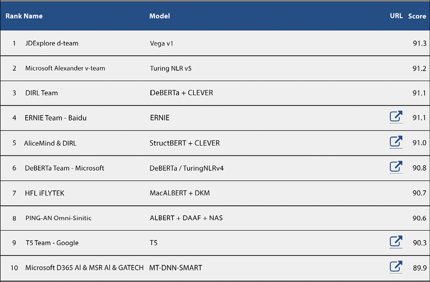
Figure 6.17: GLUE dashboard

SuperGLUE

In recent years, new models and methods for pretraining and transfer learning have driven striking performance improvements across a range of language understanding tasks. The GLUE benchmark offers a single-number metric that summarizes progress on a diverse set of such tasks, but performance on the benchmark has recently come close to the level of non-expert humans, suggesting limited headroom for further research.

SuperGLUE is a new benchmark styled after GLUE with a new set of more difficult language understanding tasks, improved resources, and a new public leaderboard. Figure 6.18 is the SuperGLUE leaderboard from March 2022:

Figure 6.18: SuperGLUE leaderboard

SQuAD

SQuAD is a dataset used to evaluate questions and answers, https://rajpurkar.github.io/SQuAD-explorer/. Specifically, the Stanford Question Answering Dataset (SQuAD) is a reading comprehension dataset, consisting of questions posed by crowdworkers on a set of Wikipedia articles, where the answer to every question is a segment of text, or span, from the corresponding reading passage, otherwise the question might be unanswerable.

SQuAD2.0 combines the 100,000 questions in SQuAD1.1 with over 50,000 unanswerable questions written adversarially by crowdworkers to look similar to answerable ones. To do well on SQuAD2.0, systems must not only answer questions when possible but also determine when no answer is supported by the paragraph and abstain from answering.

RACE

The ReAding Comprehension dataset from Examinations (RACE) dataset is a machine reading comprehension dataset consisting of 27,933 passages and 97,867 questions from English exams, targeting Chinese students aged 12-18. RACE consists of two subsets, RACE-M and RACE-H, from middle school and high school exams, respectively. RACE-M has 28,293 questions and RACE-H has 69,574. Each question is associated with four candidate answers, one of which is correct. The data generation process of RACE differs from most machine reading comprehension datasets. Instead of generating questions and answers by heuristics or crowdsourcing, questions in RACE are specifically designed for testing human reading skills and are created by domain experts. RACE is available at https://www.cs.cmu.edu/~glai1/data/race/. Figure 6.19 shows the RACE leaderboard:

Figure 6.19: RACE leaderboard

NLP-progress

NLP-progress is a repository, made to track progress in NLP, including the datasets and the current state-of-the-art models for the most common NLP tasks. The site aims to track the progress in NLP and gives an overview of the state-of-the-art models across the most common NLP tasks and their corresponding datasets. NLP-progress aims to cover both traditional and core NLP tasks such as dependency parsing and part-of-speech tagging as well as more recent ones such as reading comprehension and natural language inference. If you need a good starting point to find quality metrics for your task, then http://nlpprogress.com/ is the place to start with.

Size

The previous section provided an overview of quality metrics. This section focuses on the number of parameters used in various transformer architectures. As shown in Figure 6.20, there has been a race to increase transformers’ size during the last few years. Back in 2018, BERT’s size was about 340 million parameters, then in 2021, T5 reached 11 billion, and Megatron passed 500 billion. The very recent Switch Transformer has more than one trillion parameters and there is an expectation that soon we will see the first model with 100 trillion parameters. Indeed, there is evidence that the larger the model is the merrier, which can memorize information and generalize. However, training such large models requires massive computational resources:

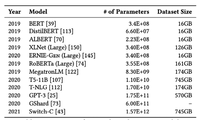
Figure 6.20: Transformers’ size in billions of parameters

Trillion parameter transformers are on their way!

In fact, the paper https://arxiv.org/pdf/1906.02243.pdf warns about the sustainability impact of training large models (see Figure 6.21) in terms of both cloud computing cost and CO2 emissions:

Figure 6.21: Estimated cost of training a model in terms of CO2 emissions (lbs) and cloud computing cost (USD) - source: https://arxiv.org/pdf/1906.02243.pdf

So, size is not the only factor that enables the quality of transformers to improve, as larger sizes can in reality give only marginal gains and require significant computational resources for training.

Larger doesn’t always mean better

At the beginning of 2022, a new trend is emerging consisting of a hybrid approach where large models are used together with a more traditional retrieval mechanism. We discussed this approach earlier in the chapter when we discussed RETRO. The RETRO language model implements a learning scheme based on the use of external memory. DeepMind claimed that RETRO (or “Retrieval Enhanced Transformer”) performs like a neural network 25 times its size. GPT-3 has 175 billion parameters and RETRO uses just seven billion of them. Of course, this requires less time, energy, and computing power to train.

Cost of serving

The cost of serving a model depends on many factors and it’s difficult to estimate it without making reasonable assumptions. Of course, serving is a function of the number of parameters in the model. In addition, the number of queries submitted to the model for inference is another factor. Then, it’s important to consider whether or not a cloud provider manages the model or is served in your on-prem infrastructure. In this context, it might be useful to remember that MLOps (see https://en.wikipedia.org/wiki/MLOps) is the process of developing a machine learning model and deploying it as a production system. Of course, MLOps’ best practices might be adopted to optimize the costs of serving.

In this section, we have seen some key factors used to evaluate transformers, namely quality, size, and cost of serving. The list is clearly not inclusive, and a proper evaluation will take into account what the optimal tradeoff is among these factors. In the next section, we will discuss optimization.

Optimization

Optimizing a transformer involves building lightweight, responsive, and energy-efficient models. Let’s see the most common ideas adopted to optimize a model.

Quantization

The key idea behind quantization is to approximate the weights of a network with a smaller precision. The idea is very simple, but it works quite well in practice. If you are interested in knowing more, we recommend the paper A Survey of Quantization Methods for Efficient Neural Network Inference, by Amir Gholami et al., https://arxiv.org/pdf/2103.13630.pdf.

Weight pruning

The key idea behind weight pruning is to remove some connections in the network. Magnitude-based weight pruning tends to zero out of model weights during training to increase model sparsity. This simple technique has benefits both in terms of model size and in cost of serving, as magnitude-based weight pruning gradually zeroes out of model weights during the training process to achieve model sparsity. Sparse models are easier to compress, and we can skip the zeroes during inference for latency improvements.

One more time, weight pruning is about tradeoffs as it might generate some quality losses although normally, they are rather small. If you are interested to know more, please have a look at the TensorFlow guide about pruning: https://www.tensorflow.org/model_optimization/guide/pruning/comprehensive_guide.

Distillation

The key idea behind knowledge distillation is to have a small model trained to reproduce the behavior of a larger model. This compression technique is sometimes referred to as teacher-student learning. The seminal paper you should check is Distilling the Knowledge in a Neural Network by Geoffrey Hinton, Oriol Vinyals, and Jeff Dean, https://arxiv.org/abs/1503.02531.

During the last few years, we have seen a number of distilled transformers. For instance, DistilBERT is a small, fast, cheap, and light transformer model based on the BERT architecture. Knowledge distillation is performed during the pretraining phase to reduce the size of a BERT model by 40%. Hugging Face has some ready-to-use Python scripts for distilling seq2seq T5 models available online at https://github.com/huggingface/transformers/tree/master/examples/research_projects/seq2seq-distillation. Using the script is quite intuitive:

python distillation.py --teacher t5-small --data_dir cnn_dm 
--student_decoder_layers 3 --student_encoder_layers 6 --tokenizer_name t5-small 
--learning_rate=3e-4 --freeze_encoder --no_teacher --freeze_embeds 
--do_train --train_batch_size 32 
--do_predict 
--model_name_or_path t5-small --eval_beams 2 --eval_max_gen_length 142 
--val_check_interval 0.25 --n_val 1000 
--output_dir distilt5 --gpus 1 --logger_name wandb

In this section, we have discussed a few techniques used to optimize transformers, namely quantization, weight pruning, and distillation. In the next section, we will discuss common pitfalls for transformers.

Common pitfalls: dos and don’ts

In this section, we will give five dos and a few don’ts that are typically recommended when dealing with transformers.

Dos

Let’s start with recommended best practices:

• Do use pretrained large models. Today, it is almost always convenient to start from an already available pretrained model such as T5, instead of training your transformer from scratch. If you use a pretrained model, you for sure stand on the giant’s shoulders; think about it!
• Do start with few-shot learning. When you start working with transformers, it’s always a good idea to start with a pretrained model and then perform a lightweight few-shot learning step. Generally, this would improve the quality of results without high computational costs.
• Do use fine-tuning on your domain data and on your customer data. After playing with pretraining models and few-shot learning, you might consider doing a proper fine-tuning on your own proprietary data or on publicly available data for your domain of interest
• Get yourself familiar with transformers’ libraries. Hugging Face or TFHub provide already available state-of-the-art implementations of almost all the known transformers. It might be useful to start from there unless you either have some very peculiar needs or are doing some innovative research work.
• Get yourself familiar with the most commonly used evaluation metrics. When you use transformers, it is ideal to take into account the tradeoff faced in terms of quality, size, cost of serving, and many other factors.

Don’ts

Now let’s have a look at some of the pitfalls that you should avoid!

• Do not use very large models as a starting point. Large models come with a cost in terms of training and serving. You will need significant resources to fine-tune, and you might pay high costs for serving each query. It might be better to start with smaller models and understand whether they are useful for your quality needs.
• Do not use unoptimized models. Nowadays, quantization, pruning, and distillation are standard techniques that need to be used by any transformer system that is put into production.

In this section, we have seen some of the best practices for transformers. In the next section, we will talk about future solutions for these architectures.

The future of transformers

Transformers found their initial applications in NLP tasks, while CNNs are typically used for image processing systems. Recently, transformers have started to be successfully used for vision processing tasks. Vision transformers compute relationships among pixels in various small sections of an image (for example, 16 x 16 pixels). This approach has been proposed in the seminar paper An Image is Worth 16x16 Words: Transformers for Image Recognition at Scale by Alexey Dosovitskiy et al., https://arxiv.org/abs/2010.11929, to make the attention computation feasible.

Vision transformers (ViTs) are today used for complex applications such as autonomous driving. Tesla’s engineers showed that their Tesla Autopilot uses a transformer on the multi-camera system in cars. Of course, ViTs are also used for more traditional computer vision tasks, including but not limited to image classification, object detection, video deepfake detection, image segmentation, anomaly detection, image synthesis, and cluster analysis. The results are frequently better than CNNs.

Another direction to consider is few-shot learning. Few-shot learning refers to the practice of feeding a machine learning model with a very small amount of training data to guide its predictions, like a few examples at inference time, as opposed to standard fine-tuning techniques that require a relatively large amount of training data for the pretrained model to adapt to the desired task with accuracy.

So, a model trained for a specific task can be reused for completely new tasks with very marginal costs. For instance, suppose we train a text model to generate text. Then, we want to perform new tasks such as translation or summarization. What we do is give a few examples of translations (say with pairs of text manually translated), or a few examples of summarization (again a few pairs). That’s it, no need for retraining or fine-tuning training.

Since FSL is proven to work well in a number of increasing domains, don’t be surprised that the training phase will be less and less relevant for future AI. More information can be found in this paper, Code Generation Tools (Almost) for Free? A Study of Few-Shot, Pre-Trained Language Models on Code by Patrick Bareiß, Beatriz Souza, Marcelo d’Amorim, and Michael Pradel. The authors propose to use FSL to generate programming code with CodeGen, an open source mode for program synthesis (see https://github.com/salesforce/CodeGen).

Summary

In this chapter, we discussed transformers, a deep learning architecture that has revolutionized the traditional natural language processing field. We started reviewing the key intuitions behind the architecture, and various categories of transformers together with a deep dive into the most popular models. Then, we focused on implementations both based on vanilla architecture and on popular libraries such as Hugging Face and TFHub. After that, we briefly discussed evaluation, optimization, and some of the best practices commonly adopted when using transformers. The last section was devoted to reviewing how transformers can be used to perform computer vision tasks, a totally different domain from NLP. That requires a careful definition of the attention mechanism. In the end, attention is all you need! And at the core of attention is nothing more than the cosine similarity between vectors.

The next chapter is devoted to unsupervised learning.

Join our book’s Discord space

Join our Discord community to meet like-minded people and learn alongside more than 2000 members at: https://packt.link/keras