5

Recurrent Neural Networks

In Chapter 3, we learned about Convolutional Neural Networks (CNNs) and saw how they exploit the spatial geometry of their inputs. For example, CNNs for images apply convolutions to initially small patches of the image, and progress to larger and larger areas of the image using pooling operations. Convolutions and pooling operations for images are in two dimensions: the width and the height. For audio and text streams, one-dimensional convolution and pooling operations are applied along the time dimension, and for video streams, these operations are applied in three dimensions: along the height, width, and time dimensions.

In this chapter, we will focus on Recurrent Neural Networks (RNNs), a class of neural networks that is popularly used on text inputs. RNNs are very flexible and have been used to solve problems such as speech recognition, language modeling, machine translation, sentiment analysis, and image captioning, to name a few. RNNs exploit the sequential nature of their input. Sequential inputs could be text, speech, time series, and anything else where the occurrence of an element in a sequence is dependent on the elements that came before it. In this chapter, we will see examples of various RNNs and learn how to implement them with TensorFlow.

We will first look at the internals of a basic RNN cell and how it deals with these sequential dependencies in the input. We will also learn about some limitations of the basic RNN cell (implemented as SimpleRNN in Keras) and see how two popular variants of the SimpleRNN cell – the Long Short-Term Memory (LSTM) and the Gated Recurrent Unit (GRU) – overcome this limitation.

We will then zoom out one level and consider the RNN layer itself, which is just the RNN cell applied to every time step. An RNN can be thought of as a graph of RNN cells, where each cell performs the same operation on successive elements of the sequence. We will describe some simple modifications to improve performance, such as making the RNN bidirectional and/or stateful.

Finally, we look at some standard RNN topologies and the kind of applications they can be used to solve. RNNs can be adapted to different types of applications by rearranging the cells in the graph. We will see some examples of these configurations and how they are used to solve specific problems. We will also consider the sequence-to-sequence (or seq2seq) architecture, which has been used with great success in machine translation and various other fields. We will then look at what an attention mechanism is, and how it can be used to improve the performance of sequence-to-sequence architectures.

In this chapter, we will cover the following topics:

• The basic RNN cell
• RNN cell variants
• RNN variants
• RNN topologies
• Encoder-decoder architectures – seq2seq
• Attention mechanism

It is often said that a journey of a thousand miles starts with a single step, so in that spirit, let’s begin our study of RNNs by first considering the RNN cell.

The basic RNN cell

Traditional multilayer perceptron neural networks make the assumption that all inputs are independent of each other. This assumption is not true for many types of sequence data. For example, words in a sentence, musical notes in a composition, stock prices over time, or even molecules in a compound are examples of sequences where an element will display a dependence on previous elements.

RNN cells incorporate this dependence by having a hidden state, or memory, that holds the essence of what has been seen so far. The value of the hidden state at any point in time is a function of the value of the hidden state at the previous time step, and the value of the input at the current time step, that is:

Here, h_t and h_t-1 are the values of the hidden states at the time t and t-1 respectively, and x_t is the value of the input at time t. Notice that the equation is recursive, that is, h_t-1 can be represented in terms of h_t-2 and x_t-1, and so on, until the beginning of the sequence. This is how RNNs encode and incorporate information from arbitrarily long sequences.

We can also represent the RNN cell graphically, as shown in Figure 5.1(a). At time t, the cell has an input x(t) and output y(t). Part of the output y(t) (represented by the hidden state h_t) is fed back into the cell for use at a later time step t+1.

Just as in a traditional neural network, where the learned parameters are stored as weight matrices, the RNN’s parameters are defined by the three weight matrices U, V, and W, corresponding to the weights of the input, output, and hidden states respectively:

Figure 5.1: (a) Schematic of an RNN cell; (b) the RNN cell unrolled

Figure 5.1(b) shows the same RNN in an “unrolled view.” Unrolling just means that we draw the network out for the complete sequence. The network shown here has three time steps, suitable for processing three element sequences. Note that the weight matrices U, V, and W, that we spoke about earlier, are shared between each of the time steps. This is because we are applying the same operation to different inputs at each time step. Being able to share these weights across all the time steps greatly reduces the number of parameters that the RNN needs to learn.

We can also describe the RNN as a computation graph in terms of equations. The internal state of the RNN at a time t is given by the value of the hidden vector h(t), which is the sum of the weight matrix W and the hidden state h_t-1 at time t-1, and the product of the weight matrix U and the input x_t at time t, passed through a tanh activation function. The choice of tanh over other activation functions such as sigmoid has to do with it being more efficient for learning in practice and helps combat the vanishing gradient problem, which we will learn about later in the chapter.

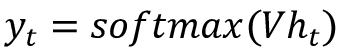
The output vector y_t at time t is the product of the weight matrix V and the hidden state h_t, passed through a softmax activation, such that the resulting vector is a set of output probabilities:

Keras provides the SimpleRNN recurrent layer that incorporates all the logic we have seen so far, as well as the more advanced variants such as LSTM and GRU, which we will learn about later in this chapter. Strictly speaking, it is not necessary to understand how they work to start building with them.

However, an understanding of the structure and equations is helpful when you need to build your own specialized RNN cell to overcome a specific problem.

Now that we understand the flow of data forward through the RNN cell, that is, how it combines its input and hidden states to produce the output and the next hidden state, let us now examine the flow of gradients in the reverse direction. This is a process called Backpropagation Through Time (BPTT).

Backpropagation through time (BPTT)

Just like traditional neural networks, training RNNs also involves the backpropagation of gradients. The difference, in this case, is that since the weights are shared by all time steps, the gradient at each output depends not only on the current time step but also on the previous ones. This process is called backpropagation through time [11]. Because the weights U, V, and W, are shared across the different time steps in the case of RNNs, we need to sum up the gradients across the various time steps in the case of BPTT. This is the key difference between traditional backpropagation and BPTT.

Consider the RNN with five time steps shown in Figure 5.2. During the forward pass, the network produces predictions ŷ_t at time t that are compared with the label y_t to compute a loss L_t. During backpropagation (shown by the dotted lines), the gradients of the loss with respect to the weights U, V, and W, are computed at each time step and the parameters updated with the sum of the gradients:

Figure 5.2: Backpropagation through time

The following equation shows the gradient of the loss with respect to W. We focus on this weight because it is the cause of the phenomenon known as the vanishing and exploding gradient problem.

This problem manifests as the gradients of the loss approaching either zero or infinity, making the network hard to train. To understand why this happens, consider the equation of the SimpleRNN we saw earlier; the hidden state h_t is dependent on h_t-1, which in turn is dependent on h_t-2, and so on:

Let’s now see what happens to this gradient at time step t=3. By the chain rule, the gradient of the loss with respect to W can be decomposed to a product of three sub-gradients. The gradient of the hidden state h₂ with respect to W can be further decomposed as the sum of the gradient of each hidden state with respect to the previous one. Finally, each gradient of the hidden state with respect to the previous one can be further decomposed as the product of gradients of the current hidden state against the previous hidden state:

Similar calculations are done to compute the gradient of the other losses L₀ through L₄ with respect to W, and sum them up into the gradient update for W. We will not explore the math further in this book, but this WildML blog post [12] has a very good explanation of BPTT, including a more detailed derivation of the math behind the process.

Vanishing and exploding gradients

The reason BPTT is particularly sensitive to the problem of vanishing and exploding gradients comes from the product part of the expression representing the final formulation of the gradient of the loss with respect to W. Consider the case where the individual gradients of a hidden state with respect to the previous one are less than 1.

As we backpropagate across multiple time steps, the product of gradients becomes smaller and smaller, ultimately leading to the problem of vanishing gradients. Similarly, if the gradients are larger than 1, the products get larger and larger, and ultimately lead to the problem of exploding gradients.

Of the two, exploding gradients are more easily detectable. The gradients will become very large and turn into Not a Number (NaN), and the training process will crash. Exploding gradients can be controlled by clipping them at a predefined threshold [13]. TensorFlow 2.0 allows you to clip gradients using the clipvalue or clipnorm parameter during optimizer construction, or by explicitly clipping gradients using tf.clip_by_value.

The effect of vanishing gradients is that gradients from time steps that are far away do not contribute anything to the learning process, so the RNN ends up not learning any long-range dependencies. While there are a few approaches toward minimizing the problem, such as proper initialization of the W matrix, more aggressive regularization, using ReLU instead of tanh activation, and pretraining the layers using unsupervised methods, the most popular solution is to use LSTM or GRU architectures, both of which will be explained shortly. These architectures have been designed to deal with vanishing gradients and learn long-term dependencies more effectively.

RNN cell variants

In this section, we’ll look at some cell variants of RNNs. We’ll begin by looking at a variant of the SimpleRNN cell: the LSTM RNN.

Long short-term memory (LSTM)

The LSTM is a variant of the SimpleRNN cell that is capable of learning long-term dependencies. LSTMs were first proposed by Hochreiter and SchmidHuber [14] and refined by many other researchers. They work well on a large variety of problems and are the most widely used RNN variant.

We have seen how the SimpleRNN combines the hidden state from the previous time step and the current input through a tanh layer to implement recurrence. LSTMs also implement recurrence in a similar way, but instead of a single tanh layer, there are four layers interacting in a very specific way. Figure 5.3 illustrates the transformations that are applied in the hidden state at time step t.

The diagram looks complicated, but let’s look at it component by component. The line across the top of the diagram is the cell state c, representing the internal memory of the unit.

The line across the bottom is the hidden state h, and the i, f, o, and g gates are the mechanisms by which the LSTM works around the vanishing gradient problem. During training, the LSTM learns the parameters of these gates:

Figure 5.3: An LSTM cell

An alternative way to think about how these gates work inside an LSTM cell is to consider the equations of the cell. These equations describe how the value of the hidden state h_t at time t is calculated from the value of hidden state h_t-1 at the previous time step. In general, the equation-based description tends to be clearer and more concise and is usually the way a new cell design is presented in academic papers. Diagrams, when provided, may or may not be comparable to the ones you saw earlier. For these reasons, it usually makes sense to learn to read the equations and visualize the cell design. To that end, we will describe the other cell variants in this book using equations only.

The set of equations representing an LSTM is shown as follows:

Here, i, f, and o are the input, forget, and output gates. They are computed using the same equations but with different parameter matrices W_i, U_i, W_f, U_f, and W_o, U_o. The sigmoid function modulates the output of these gates between 0 and 1, so the output vectors produced can be multiplied element-wise with another vector to define how much of the second vector can pass through the first one.

The forget gate defines how much of the previous state h_t-1 you want to allow to pass through. The input gate defines how much of the newly computed state for the current input x_t you want to let through, and the output gate defines how much of the internal state you want to expose to the next layer. The internal hidden state g is computed based on the current input x_t and the previous hidden state h_t-1. Notice that the equation for g is identical to that of the SimpleRNN, except that in this case, we will modulate the output by the output of input vector i.

Given i, f, o, and g, we can now calculate the cell state c_t at time t as the cell state c_t-1 at time (t-1) multiplied by the value of the forget gate g, plus the state g multiplied by the input gate i. This is basically a way to combine the previous memory and the new input – setting the forget gate to 0 ignores the old memory and setting the input gate to 0 ignores the newly computed state. Finally, the hidden state h_t at time t is computed as the memory c_t at time t, with the output gate o.

One thing to realize is that the LSTM is a drop-in replacement for a SimpleRNN cell; the only difference is that LSTMs are resistant to the vanishing gradient problem. You can replace an RNN cell in a network with an LSTM without worrying about any side effects. You should generally see better results along with longer training times.

TensorFlow 2.0 also provides a ConvLSTM2D implementation based on the paper by Shi, et al. [18], where the matrix multiplications are replaced by convolution operators.

If you would like to learn more about LSTMs, please take a look at the WildML RNN tutorial [15] and Christopher Olah’s blog post [16]. The first covers LSTMs in somewhat greater detail, and the second takes you step by step through the computations in a very visual way.

Now that we have covered LTSMs, we will cover the other popular RNN cell architecture – GRUs.

Gated recurrent unit (GRU)

The GRU is a variant of the LSTM and was introduced by Cho, et al [17]. It retains the LSTM’s resistance to the vanishing gradient problem, but its internal structure is simpler, and is, therefore, faster to train, since fewer computations are needed to make updates to its hidden state.

Instead of the input (i), forgot (f), and output (o) gates in the LSTM cell, the GRU cell has two gates, an update gate z and a reset gate r. The update gate defines how much previous memory to keep around, and the reset gate defines how to combine the new input with the previous memory. There is no persistent cell state distinct from the hidden state as it is in LSTM.

The GRU cell defines the computation of the hidden state h_t at time t from the hidden state h_t-1 at the previous time step using the following set of equations:

The outputs of the update gate z and the reset gate r are both computed using a combination of the previous hidden state h_t-1 and the current input x_t. The sigmoid function modulates the output of these functions between 0 and 1. The cell state c is computed as a function of the output of the reset gate r and input x_t. Finally, the hidden state h_t at time t is computed as a function of the cell state c and the previous hidden state h_t-1. The parameters W_z, U_z, W_r, U_r, and W_c, U_c, are learned during training.

Similar to LSTM, TensorFlow 2.0 (tf.keras) provides an implementation for the basic GRU layer as well, which is a drop-in replacement for the RNN cell.

Peephole LSTM

The peephole LSTM is an LSTM variant that was first proposed by Gers and Schmidhuber [19]. It adds “peepholes” to the input, forget, and output gates, so they can see the previous cell state c_t-1. The equations for computing the hidden state h_t, at time t, from the hidden state h_t-1 at the previous time step, in a peephole LSTM are shown next.

Notice that the only difference from the equations for the LSTM is the additional c_t-1 term for computing outputs of the input (i), forget (f), and output (o) gates:

TensorFlow 2.0 provides an experimental implementation of the peephole LSTM cell. To use this in your own RNN layers, you will need to wrap the cell (or list of cells) in the RNN wrapper, as shown in the following code snippet:

hidden_dim = 256
peephole_cell = tf.keras.experimental.PeepholeLSTMCell(hidden_dim)
rnn_layer = tf.keras.layers.RNN(peephole_cell)

In the previous section, we saw some RNN cell variants that were developed to target specific inadequacies of the basic RNN cell. In the next section, we will look at variations in the architecture of the RNN network itself, which were built to address specific use cases.

RNN variants

In this section, we will look at a couple of variations of the basic RNN architecture that can provide performance improvements in some specific circumstances. Note that these strategies can be applied to different kinds of RNN cells, as well as for different RNN topologies, which we will learn about later.

Bidirectional RNNs

We have seen how, at any given time step t, the output of the RNN is dependent on the outputs at all previous time steps. However, it is entirely possible that the output is also dependent on the future outputs as well. This is especially true for applications such as natural language processing where the attributes of the word or phrase we are trying to predict may be dependent on the context given by the entire enclosing sentence, not just the words that came before it.

This problem can be solved using a bidirectional LSTM (see Figure 5.4), also called biLSTM, which is essentially two RNNs stacked on top of each other, one reading the input from left to right, and the other reading the input from the right to the left.

The output at each time step will be based on the hidden state of both RNNs. Bidirectional RNNs allow the network to place equal emphasis on the beginning and end of the sequence, and typically result in performance improvements:

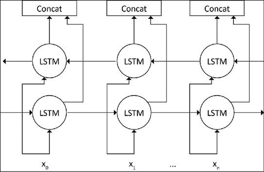
Figure 5.4: Bidirectional LSTM

TensorFlow 2.0 provides support for bidirectional RNNs through a bidirectional wrapper layer. To make an RNN layer bidirectional, all that is needed is to wrap the layer with this wrapper layer, which is shown as follows. Since the output of each pair of cells in the left and right LSTM in the biLSTM pair are concatenated (see Figure 5.4), it needs to return output from each cell. Hence, we set return_sequences to True (the default is False meaning that the output is only returned from the last cell in the LSTM):

self.lstm = tf.keras.layers.Bidirectional(
    tf.keras.layers.LSTM(10, return_sequences=True, 
        input_shape=(5, 10))
)

The next major RNN variation we will look at is the Stateful RNN.

Stateful RNNs

RNNs can be stateful, which means that they can maintain state across batches during training. That is, the hidden state computed for a batch of training data will be used as the initial hidden state for the next batch of training data. However, this needs to be explicitly set, since TensorFlow 2.0 (tf.keras) RNNs are stateless by default, and resets the state after each batch. Setting an RNN to be stateful means that it can build state across its training sequence and even maintain that state when doing predictions.

The benefits of using stateful RNNs are smaller network sizes and/or lower training times. The disadvantage is that we are now responsible for training the network with a batch size that reflects the periodicity of the data and resetting the state after each epoch. In addition, data should not be shuffled while training the network since the order in which the data is presented is relevant for stateful networks.

To set an RNN layer as stateful, set the named variable stateful to True. In our example of a one-to-many topology for learning how to generate text, we provide an example of using a stateful RNN. Here, we train using data consisting of contiguous text slices, so setting the LSTM to stateful means that the hidden state generated from the previous text chunk is reused for the current text chunk.

In the next section on RNN topologies, we will look at different ways to set up the RNN network for different use cases.

RNN topologies

We have seen examples of how MLP and CNN architectures can be composed to form more complex networks. RNNs offer yet another degree of freedom, in that they allow sequence input and output. This means that RNN cells can be arranged in different ways to build networks that are adapted to solve different types of problems. Figure 5.5 shows five different configurations of inputs, hidden layers, and outputs.

Of these, the first one (one-to-one) is not interesting from a sequence processing point of view, as it can be implemented as a simple dense network with one input and one output.

The one-to-many case has a single input and outputs a sequence. An example of such a network might be a network that can generate text tags from images [6], containing short text descriptions of different aspects of the image. Such a network would be trained with image input and labeled sequences of text representing the image tags:

Figure 5.5: Common RNN topologies

The many-to-one case is the reverse; it takes a sequence of tensors as input but outputs a single tensor. Examples of such networks would be a sentiment analysis network [7], which takes as input a block of text such as a movie review and outputs a single sentiment value.

The many-to-many use case comes in two flavors. The first one is more popular and is better known as the seq2seq model. In this model, a sequence is read in and produces a context vector representing the input sequence, which is used to generate the output sequence.

The topology has been used with great success in the field of machine translation, as well as problems that can be reframed as machine translation problems. Real-life examples of the former can be found in [8, 9], and an example of the latter is described in [10].

The second many-to-many type has an output cell corresponding to each input cell. This kind of network is suited for use cases where there is a 1:1 correspondence between the input and output, such as time series. The major difference between this model and the seq2seq model is that the input does not have to be completely encoded before the decoding process begins.

In the next three sections, we provide examples of a one-to-many network that learns to generate text, a many-to-one network that does sentiment analysis, and a many-to-many network of the second type, which predicts Part-of-Speech (POS) for words in a sentence. Because of the popularity of the seq2seq network, we will cover it in more detail later in this chapter.

Example ‒ One-to-many – Learning to generate text

RNNs have been used extensively by the Natural Language Processing (NLP) community for various applications. One such application is to build language models. A language model is a model that allows us to predict the probability of a word in a text given previous words. Language models are important for various higher-level tasks such as machine translation, spelling correction, and so on.

The ability of a language model to predict the next word in a sequence makes it a generative model that allows us to generate text by sampling from the output probabilities of different words in the vocabulary. The training data is a sequence of words, and the label is the word appearing at the next time step in the sequence.

For our example, we will train a character-based RNN on the text of the children’s stories Alice in Wonderland and its sequel Through the Looking Glass by Lewis Carroll. We have chosen to build a character-based model because it has a smaller vocabulary and trains quicker. The idea is the same as training and using a word-based language model, except we will use characters instead of words. Once trained, the model can be used to generate some text in the same style.

The data for our example will come from the plain texts of two novels on the Project Gutenberg website [36]. Input to the network are sequences of 100 characters, and the corresponding output is another sequence of 100 characters, offset from the input by 1 position.

That is, if the input is the sequence [c₁, c₂, …, c_n], the output will be [c₂, c₃, …, c_n+1]. We will train the network for 50 epochs, and at the end of every 10 epochs, we will generate a fixed-size sequence of characters starting with a standard prefix. In the following example, we have used the prefix “Alice”, the name of the protagonist in our novels.

As always, we will first import the necessary libraries and set up some constants. Here, DATA_DIR points to a data folder under the location where you downloaded the source code for this chapter. CHECKPOINT_DIR is the location, a folder of checkpoints under the data folder, where we will save the weights of the model at the end of every 10 epochs:

import os
import numpy as np
import re
import shutil
import tensorflow as tf
DATA_DIR = "./data"
CHECKPOINT_DIR = os.path.join(DATA_DIR, "checkpoints")

Next, we download and prepare the data for our network to consume. The texts of both books are publicly available from the Project Gutenberg website. The tf.keras.utils.get_file() function will check to see whether the file has already been downloaded to your local drive, and if not, it will download to a datasets folder under the location of the code. We also preprocess the input a little here, removing newline and byte order mark characters from the text. This step will create the texts variable, a flat list of characters for these two books:

def download_and_read(urls):
    texts = []
    for i, url in enumerate(urls):
        p = tf.keras.utils.get_file("ex1-{:d}.txt".format(i), url,
            cache_dir=".")
        text = open(p, "r").read()
        # remove byte order mark
        text = text.replace("ufeff", "")
        # remove newlines
        text = text.replace('
', ' ')
        text = re.sub(r's+', " ", text)
        # add it to the list
        texts.extend(text)
    return texts
texts = download_and_read([
    "http://www.gutenberg.org/cache/epub/28885/pg28885.txt",
    "https://www.gutenberg.org/files/12/12-0.txt"
])

Next, we will create our vocabulary. In our case, our vocabulary contains 90 unique characters, composed of uppercase and lowercase alphabets, numbers, and special characters. We also create some mapping dictionaries to convert each vocabulary character into a unique integer and vice versa. As noted earlier, the input and output of the network is a sequence of characters.

However, the actual input and output of the network are sequences of integers, and we will use these mapping dictionaries to handle this conversion:

# create the vocabulary
vocab = sorted(set(texts))
print("vocab size: {:d}".format(len(vocab)))
# create mapping from vocab chars to ints
char2idx = {c:i for i, c in enumerate(vocab)}
idx2char = {i:c for c, i in char2idx.items()}

The next step is to use these mapping dictionaries to convert our character sequence input into an integer sequence and then into a TensorFlow dataset. Each of our sequences is going to be 100 characters long, with the output being offset from the input by 1 character position. We first batch the dataset into slices of 101 characters, then apply the split_train_labels() function to every element of the dataset to create our sequences dataset, which is a dataset of tuples of two elements, with each element of the tuple being a vector of size 100 and type tf.int64. We then shuffle these sequences and create batches of 64 tuples for each input to our network. Each element of the dataset is now a tuple consisting of a pair of matrices, each of size (64, 100) and type tf.int64:

# numericize the texts
texts_as_ints = np.array([char2idx[c] for c in texts])
data = tf.data.Dataset.from_tensor_slices(texts_as_ints)
# number of characters to show before asking for prediction
# sequences: [None, 100]
seq_length = 100
sequences = data.batch(seq_length + 1, drop_remainder=True)
def split_train_labels(sequence):
    input_seq = sequence[0:-1]
    output_seq = sequence[1:]
    return input_seq, output_seq
sequences = sequences.map(split_train_labels)
# set up for training
# batches: [None, 64, 100]
batch_size = 64
steps_per_epoch = len(texts) // seq_length // batch_size
dataset = sequences.shuffle(10000).batch(
    batch_size, drop_remainder=True)

We are now ready to define our network. As before, we define our network as a subclass of tf.keras.Model, as shown next. The network is fairly simple; it takes as input a sequence of integers of size 100 (num_timesteps) and passes them through an embedding layer so that each integer in the sequence is converted into a vector of size 256 (embedding_dim). So, assuming a batch size of 64, for our input sequence of size (64, 100), the output of the embedding layer is a matrix of shape (64, 100, 256).

The next layer is an RNN layer with 100 time steps. The implementation of RNN chosen is a GRU. This GRU layer will take, at each of its time steps, a vector of size (256,) and output a vector of shape (1024,) (rnn_output_dim). Note also that the RNN is stateful, which means that the hidden state output from the previous training epoch will be used as input to the current epoch. The return_sequences=True flag also indicates that the RNN will output at each of the time steps rather than an aggregate output at the last time steps.

Finally, each of the time steps will emit a vector of shape (1024,) into a dense layer that outputs a vector of shape (90,) (vocab_size). The output from this layer will be a tensor of shape (64, 100, 90). Each position in the output vector corresponds to a character in our vocabulary, and the values correspond to the probability of that character occurring at that output position:

class CharGenModel(tf.keras.Model):
    def __init__(self, vocab_size, num_timesteps,
            embedding_dim, **kwargs):
        super(CharGenModel, self).__init__(**kwargs)
        self.embedding_layer = tf.keras.layers.Embedding(
            vocab_size,
            embedding_dim
        )
        self.rnn_layer = tf.keras.layers.GRU(
            num_timesteps,
            recurrent_initializer="glorot_uniform",
            recurrent_activation="sigmoid",
            stateful=True,
            return_sequences=True)
        self.dense_layer = tf.keras.layers.Dense(vocab_size)
    def call(self, x):
        x = self.embedding_layer(x)
        x = self.rnn_layer(x)
        x = self.dense_layer(x)
        return x
vocab_size = len(vocab)
embedding_dim = 256
model = CharGenModel(vocab_size, seq_length, embedding_dim)
model.build(input_shape=(batch_size, seq_length))

Next, we define a loss function and compile our model. We will use the sparse categorical cross-entropy as our loss function because that is the standard loss function to use when our inputs and outputs are sequences of integers. For the optimizer, we will choose the Adam optimizer:

def loss(labels, predictions):
    return tf.losses.sparse_categorical_crossentropy(
        labels,
        predictions,
        from_logits=True
    )
model.compile(optimizer=tf.optimizers.Adam(), loss=loss)

Normally, the character at each position of the output is found by computing the argmax of the vector at that position, that is, the character corresponding to the maximum probability value. This is known as greedy search. In the case of language models where the output of one time step becomes the input to the next time step, this can lead to a repetitive output. The two most common approaches to overcome this problem are either to sample the output randomly or to use beam search, which samples from k the most probable values at each time step. Here, we will use the tf.random.categorical() function to sample the output randomly. The following function takes a string as a prefix and uses it to generate a string whose length is specified by num_chars_to_generate. The temperature parameter is used to control the quality of the predictions. Lower values will create a more predictable output.

The logic follows a predictable pattern. We convert the sequence of characters in our prefix_string into a sequence of integers, then expand_dims to add a batch dimension so the input can be passed into our model. We then reset the state of the model. This is needed because our model is stateful, and we don’t want the hidden state of the first time step in our prediction run to be carried over from the one computed during training. We then run the input through our model and get back a prediction. This is the vector of shape (90,) representing the probabilities of each character in the vocabulary appearing at the next time step. We then reshape the prediction by removing the batch dimension and dividing by the temperature, and then randomly sampling from the vector. We then set our prediction as the input of the next time step. We repeat this for the number of characters we need to generate, converting each prediction back into character form and accumulating them in a list, and returning the list at the end of the loop:

def generate_text(model, prefix_string, char2idx, idx2char,
        num_chars_to_generate=1000, temperature=1.0):
    input = [char2idx[s] for s in prefix_string]
    input = tf.expand_dims(input, 0)
    text_generated = []
    model.reset_states()
    for i in range(num_chars_to_generate):
        preds = model(input)
        preds = tf.squeeze(preds, 0) / temperature
        # predict char returned by model
        pred_id = tf.random.categorical(
            preds, num_samples=1)[-1, 0].numpy()
        text_generated.append(idx2char[pred_id])
        # pass the prediction as the next input to the model
        input = tf.expand_dims([pred_id], 0)
    return prefix_string + "".join(text_generated)

Finally, we are ready to run our training and evaluation loop. As mentioned earlier, we will train our network for 50 epochs, and at every 10-epoch interval, we will try to generate some text with the model trained so far. Our prefix at each stage is the string "Alice ". Notice that in order to accommodate a single string prefix, we save the weights after every 10 epochs and build a separate generative model with these weights but with an input shape with a batch size of 1. Here is the code to do this:

num_epochs = 50
for i in range(num_epochs // 10):
    model.fit(
        dataset.repeat(),
        epochs=10,
        steps_per_epoch=steps_per_epoch
        # callbacks=[checkpoint_callback, tensorboard_callback]
    )
    checkpoint_file = os.path.join(
        CHECKPOINT_DIR, "model_epoch_{:d}".format(i+1))
    model.save_weights(checkpoint_file)
    # create generative model using the trained model so far
    gen_model = CharGenModel(vocab_size, seq_length, embedding_dim)
    gen_model.load_weights(checkpoint_file)
    gen_model.build(input_shape=(1, seq_length))
    print("after epoch: {:d}".format(i+1)*10)
    print(generate_text(gen_model, "Alice ", char2idx, idx2char))
    print("---")

The output after the very first epoch of training contains words that are completely undecipherable:

Alice nIPJtce otaishein r. henipt il nn tu t hen mlPde hc efa hdtioDDeteeybeaewI teu"t e9B ce nd ageiw  eai rdoCr ohrSI ey Pmtte:vh ndte taudhor0-gu s5'ria,tr gn inoo luwomg Omke dee sdoohdn ggtdhiAoyaphotd t- kta e c t- taLurtn   hiisd tl'lpei od y' tpacoe dnlhr oG mGhod ut hlhoy .i, sseodli., ekngnhe idlue'aa'  ndti-rla nt d'eiAier adwe ai'otteniAidee hy-ouasq"plhgs tuutandhptiw  oohe.Rastnint:e,o odwsir"omGoeuall1*g taetphhitoge ds wr li,raa,  h$jeuorsu  h cidmdg't ku..n,HnbMAsn nsaathaa,' ase woe  ehf re ig"hTr ddloese eod,aed toe rh k. nalf bte seyr udG n,ug lei hn icuimty"onw Qee ivtsae zdrye g eut rthrer n sd,Zhqehd' sr caseruhel are fd yse e  kgeiiday odW-ldmkhNw endeM[harlhroa h Wydrygslsh EnilDnt e "lue "en wHeslhglidrth"ylds rln n iiato taue flitl nnyg ittlno re 'el yOkao itswnadoli'.dnd Akib-ehn hftwinh yd ee tosetf tonne.;egren t wf, ota nfsr, t&he desnre e" oo fnrvnse aid na tesd is ioneetIf ·itrn tttpakihc s nih'bheY ilenf yoh etdrwdplloU ooaeedo,,dre snno'ofh o epst. lahehrw 

However, after about 30 epochs of training, we begin to see words that look familiar:

Alice Red Queen. He best I had defores it,' glily do flose time it makes the talking of find a hand mansed in she loweven to the rund not bright prough: the and she a chill be the sand using that whever sullusn--the dear of asker as 'IS now-- Chich the hood." "Oh!"' '_I'm num about--again was wele after a WAG LoANDE BITTER OF HSE!0 UUL EXMENN 1*.t, this wouldn't teese to Dumark THEVER Project Gutenberg-tmy of himid out flowal woulld: 'Nis song, Eftrin in pully be besoniokinote. "Com, contimemustion--of could you knowfum to hard, she can't the with talking to alfoeys distrint, for spacemark!' 'You gake to be would prescladleding readieve other togrore what it mughturied ford of it was sen!" You squs, _It I hap: But it was minute to the Kind she notion and teem what?" said Alice, make there some that in at the shills distringulf out to the Froge, and very mind to it were it?' the King was set telm, what's the old all reads talking a minuse. "Where ream put find growned his so," _you 'Fust to t

After 50 epochs of training, the model still has trouble expressing coherent thought but has learned to spell reasonably well. What is amazing here is that the model is character-based and has no knowledge of words, yet it learns to spell words that look like they might have come from the original text:

Alice Vex her," he prope of the very managed by this thill deceed. I will ear she a much daid. "I sha?' Nets: "Woll, I should shutpelf, and now and then, cried, How them yetains, a tround her about in a shy time, I pashng round the sandle, droug" shrees went on what he seting that," said Alice. "Was this will resant again. Alice stook of in a faid.' 'It's ale. So they wentle shall kneeltie-and which herfer--the about the heald in pum little each the UKECE P@TTRUST GITE Ever been my hever pertanced to becristrdphariok, and your pringing that why the King as I to the King remark, but very only all Project Grizly: thentiused about doment,' Alice with go ould, are wayings for handsn't replied as mave about to LISTE!' (If the UULE 'TARY-HAVE BUY DIMADEANGNE'G THING NOOT,' be this plam round an any bar here! No, you're alard to be a good aftered of the sam--I canon't?" said Alice. 'It's one eye of the olleations. Which saw do it just opened hardly deat, we hastowe. 'Of coum, is tried try slowing

Generating the next character or next word in the text isn’t the only thing you can do with this sort of model. Similar models have been built to make stock price predictions [3] or generate classical music [4]. Andrej Karpathy covers a few other fun examples, such as generating fake Wikipedia pages, algebraic geometry proofs, and Linux source code in his blog post [5].

The full code for this example is available in alice_text_generator.py in the source code folder for this chapter. It can be run from the command line using the following command:

$ python alice_text_generator.py

Our next example will show an implementation of a many-to-one network for sentiment analysis.

Example ‒ Many-to-one – Sentiment analysis

In this example, we will use a many-to-one network that takes a sentence as input and predicts its sentiment as being either positive or negative. Our dataset is the Sentiment-labeled sentences dataset on the UCI Machine Learning Repository [20], a set of 3,000 sentences from reviews on Amazon, IMDb, and Yelp, each labeled with 0 if it expresses a negative sentiment, or 1 if it expresses a positive sentiment.

As usual, we will start with our imports:

import numpy as np
import os
import shutil
import tensorflow as tf
from sklearn.metrics import accuracy_score, confusion_matrix

The dataset is provided as a zip file, which expands into a folder containing three files of labeled sentences, one for each provider, with one sentence and label per line and with the sentence and label separated by the tab character. We first download the zip file, then parse the files into a list of (sentence, label) pairs:

def download_and_read(url):
    local_file = url.split('/')[-1]
    local_file = local_file.replace("%20", " ")
    p = tf.keras.utils.get_file(local_file, url,
        extract=True, cache_dir=".")
    local_folder = os.path.join("datasets", local_file.split('.')[0])
    labeled_sentences = []
    for labeled_filename in os.listdir(local_folder):
        if labeled_filename.endswith("_labelled.txt"):
            with open(os.path.join(
                    local_folder, labeled_filename), "r") as f:
                for line in f:
                    sentence, label = line.strip().split('	')
                    labeled_sentences.append((sentence, label))
    return labeled_sentences
labeled_sentences = download_and_read(      
    "https://archive.ics.uci.edu/ml/machine-learning-databases/" + 
    "00331/sentiment%20labelled%20sentences.zip")
sentences = [s for (s, l) in labeled_sentences]
labels = [int(l) for (s, l) in labeled_sentences]

Our objective is to train the model so that, given a sentence as input, it learns to predict the corresponding sentiment provided in the label. Each sentence is a sequence of words. However, to input it into the model, we have to convert it into a sequence of integers.

Each integer in the sequence will point to a word. The mapping of integers to words for our corpus is called a vocabulary. Thus, we need to tokenize the sentences and produce a vocabulary. This is done using the following code:

tokenizer = tf.keras.preprocessing.text.Tokenizer()
tokenizer.fit_on_texts(sentences)
vocab_size = len(tokenizer.word_counts)
print("vocabulary size: {:d}".format(vocab_size))
word2idx = tokenizer.word_index
idx2word = {v:k for (k, v) in word2idx.items()}

Our vocabulary consists of 5,271 unique words. It is possible to make the size smaller by dropping words that occur fewer than some threshold number of times, which can be found by inspecting the tokenizer.word_counts dictionary. In such cases, we need to add 1 to the vocabulary size for the UNK (unknown) entry, which will be used to replace every word that is not found in the vocabulary.

We also construct lookup dictionaries to convert from the word-to-word index and back. The first dictionary is useful during training to construct integer sequences to feed the network. The second dictionary is used to convert from the word index back into words in our prediction code later.

Each sentence can have a different number of words. Our model will require us to provide sequences of integers of identical length for each sentence. To support this requirement, it is common to choose a maximum sequence length that is large enough to accommodate most of the sentences in the training set. Any sentences that are shorter will be padded with zeros, and any sentences that are longer will be truncated. An easy way to choose a good value for the maximum sequence length is to look at the sentence length (as in the number of words) at different percentile positions:

seq_lengths = np.array([len(s.split()) for s in sentences])
print([(p, np.percentile(seq_lengths, p)) for p
    in [75, 80, 90, 95, 99, 100]])

This gives us the following output:

[(75, 16.0), (80, 18.0), (90, 22.0), (95, 26.0), (99, 36.0), (100, 71.0)]

As can be seen, the maximum sentence length is 71 words, but 99% of the sentences are under 36 words. If we choose a value of 64, for example, we should be able to get away with not having to truncate most of the sentences.

The preceding blocks of code can be run interactively multiple times to choose good values of vocabulary size and maximum sequence length respectively. In our example, we have chosen to keep all the words (so vocab_size = 5271), and we have set our max_seqlen to 64.

Our next step is to create a dataset that our model can consume. We first use our trained tokenizer to convert each sentence from a sequence of words (sentences) into a sequence of integers (sentences_as_ints), where each corresponding integer is the index of the word in the tokenizer.word_index. It is then truncated and padded with zeros.

The labels are also converted into a NumPy array labels_as_ints, and finally, we combine the tensors sentences_as_ints and labels_as_ints to form a TensorFlow dataset:

max_seqlen = 64
# create dataset
sentences_as_ints = tokenizer.texts_to_sequences(sentences)
sentences_as_ints = tf.keras.preprocessing.sequence.pad_sequences(
    sentences_as_ints, maxlen=max_seqlen)
labels_as_ints = np.array(labels)
dataset = tf.data.Dataset.from_tensor_slices(
    (sentences_as_ints, labels_as_ints))

We want to set aside 1/3 of the dataset for evaluation. Of the remaining data, we will use 10% as an inline validation dataset, which the model will use to gauge its own progress during training, and the remaining as the training dataset. Finally, we create batches of 64 sentences for each dataset:

dataset = dataset.shuffle(10000)
test_size = len(sentences) // 3
val_size = (len(sentences) - test_size) // 10
test_dataset = dataset.take(test_size)
val_dataset = dataset.skip(test_size).take(val_size)
train_dataset = dataset.skip(test_size + val_size)
batch_size = 64
train_dataset = train_dataset.batch(batch_size)
val_dataset = val_dataset.batch(batch_size)
test_dataset = test_dataset.batch(batch_size)

Next, we define our model. As you can see, the model is fairly straightforward, each input sentence is a sequence of integers of size max_seqlen (64). This is input into an embedding layer that converts each word into a vector given by the size of the vocabulary + 1. The additional word is to account for the padding integer 0 that was introduced during the pad_sequences() call above. The vector at each of the 64 time steps is then fed into a bidirectional LSTM layer, which converts each word into a vector of size (64,). The output of the LSTM at each time step is fed into a dense layer, which produces a vector of size (64,) with ReLU activation. The output of this dense layer is then fed into another dense layer, which outputs a vector of (1,) at each time step, modulated through a sigmoid activation.

The model is compiled with the binary cross-entropy loss function and the Adam optimizer, and then trained over 10 epochs:

class SentimentAnalysisModel(tf.keras.Model):
    def __init__(self, vocab_size, max_seqlen, **kwargs):
        super(SentimentAnalysisModel, self).__init__(**kwargs)
        self.embedding = tf.keras.layers.Embedding(
            vocab_size, max_seqlen)
        self.bilstm = tf.keras.layers.Bidirectional(
            tf.keras.layers.LSTM(max_seqlen)
        )
        self.dense = tf.keras.layers.Dense(64, activation="relu")
        self.out = tf.keras.layers.Dense(1, activation="sigmoid")
    def call(self, x):
        x = self.embedding(x)
        x = self.bilstm(x)
        x = self.dense(x)
        x = self.out(x)
        return x
model = SentimentAnalysisModel(vocab_size+1, max_seqlen)
model.build(input_shape=(batch_size, max_seqlen))
model.summary()
# compile
model.compile(
    loss="binary_crossentropy",
    optimizer="adam",
    metrics=["accuracy"]
)
# train
data_dir = "./data"
logs_dir = os.path.join("./logs")
best_model_file = os.path.join(data_dir, "best_model.h5")
checkpoint = tf.keras.callbacks.ModelCheckpoint(best_model_file,
    save_weights_only=True,
    save_best_only=True)
tensorboard = tf.keras.callbacks.TensorBoard(log_dir=logs_dir)
num_epochs = 10
history = model.fit(train_dataset, epochs=num_epochs,
    validation_data=val_dataset,
    callbacks=[checkpoint, tensorboard])

As you can see from the output, the training set accuracy goes to 99.8% and the validation set accuracy goes to about 78.5%. Having a higher accuracy over the training set is expected since the model was trained on this dataset. You can also look at the following loss plot to see exactly where the model starts overfitting on the training set. Notice that the training loss keeps going down, but the validation loss comes down initially and then starts going up. It is at the point where it starts going up that we know that the model overfits on the training set:

Epoch 1/10
29/29 [==============================] - 7s 239ms/step - loss: 0.6918 - accuracy: 0.5148 - val_loss: 0.6940 - val_accuracy: 0.4750
Epoch 2/10
29/29 [==============================] - 3s 98ms/step - loss: 0.6382 - accuracy: 0.5928 - val_loss: 0.6311 - val_accuracy: 0.6000
Epoch 3/10
29/29 [==============================] - 3s 100ms/step - loss: 0.3661 - accuracy: 0.8250 - val_loss: 0.4894 - val_accuracy: 0.7600
Epoch 4/10
29/29 [==============================] - 3s 99ms/step - loss: 0.1567 - accuracy: 0.9564 - val_loss: 0.5469 - val_accuracy: 0.7750
Epoch 5/10
29/29 [==============================] - 3s 99ms/step - loss: 0.0768 - accuracy: 0.9875 - val_loss: 0.6197 - val_accuracy: 0.7450
Epoch 6/10
29/29 [==============================] - 3s 100ms/step - loss: 0.0387 - accuracy: 0.9937 - val_loss: 0.6529 - val_accuracy: 0.7500
Epoch 7/10
29/29 [==============================] - 3s 99ms/step - loss: 0.0215 - accuracy: 0.9989 - val_loss: 0.7597 - val_accuracy: 0.7550
Epoch 8/10
29/29 [==============================] - 3s 100ms/step - loss: 0.0196 - accuracy: 0.9987 - val_loss: 0.6745 - val_accuracy: 0.7450
Epoch 9/10
29/29 [==============================] - 3s 99ms/step - loss: 0.0136 - accuracy: 0.9962 - val_loss: 0.7770 - val_accuracy: 0.7500
Epoch 10/10
29/29 [==============================] - 3s 99ms/step - loss: 0.0062 - accuracy: 0.9988 - val_loss: 0.8344 - val_accuracy: 0.7450

Figure 5.6 shows TensorBoard plots of accuracy and loss for the training and validation datasets:

Figure 5.6: Accuracy and loss plots from TensorBoard for sentiment analysis network training

Our checkpoint callback has saved the best model based on the lowest value of validation loss, and we can now reload this for evaluation against our held out test set:

best_model = SentimentAnalysisModel(vocab_size+1, max_seqlen)
best_model.build(input_shape=(batch_size, max_seqlen))
best_model.load_weights(best_model_file)
best_model.compile(
    loss="binary_crossentropy",
    optimizer="adam",
    metrics=["accuracy"]
)

The easiest high-level way to evaluate a model against a dataset is to use the model.evaluate() call:

test_loss, test_acc = best_model.evaluate(test_dataset)
print("test loss: {:.3f}, test accuracy: {:.3f}".format(
    test_loss, test_acc))

This gives us the following output:

test loss: 0.487, test accuracy: 0.782

We can also use model.predict() to retrieve our predictions and compare them individually to the labels and use external tools (from scikit-learn, for example) to compute our results:

labels, predictions = [], []
idx2word[0] = "PAD"
is_first_batch = True
for test_batch in test_dataset:
   inputs_b, labels_b = test_batch
   pred_batch = best_model.predict(inputs_b)
   predictions.extend([(1 if p > 0.5 else 0) for p in pred_batch])
   labels.extend([l for l in labels_b])
   if is_first_batch:
       # print first batch of label, prediction, and sentence
       for rid in range(inputs_b.shape[0]):
           words = [idx2word[idx] for idx in inputs_b[rid].numpy()]
           words = [w for w in words if w != "PAD"]
           sentence = " ".join(words)
           print("{:d}	{:d}	{:s}".format(
               labels[rid], predictions[rid], sentence))
       is_first_batch = False
print("accuracy score: {:.3f}".format(accuracy_score(labels, predictions)))
print("confusion matrix")
print(confusion_matrix(labels, predictions))

For the first batch of 64 sentences in our test dataset, we reconstruct the sentence and display the label (first column) as well as the prediction from the model (second column). Here, we show the top 10 sentences. As you can see, the model gets it right for most sentences on this list:

LBL  PRED  SENT
1     1    one of my favorite purchases ever
1     1    works great
1     1    our waiter was very attentive friendly and informative
0     0    defective crap
0     1    and it was way to expensive
0     0    don't waste your money
0     0    friend's pasta also bad he barely touched it
1     1    it's a sad movie but very good
0     0    we recently witnessed her poor quality of management towards other guests as well
0     1    there is so much good food in vegas that i feel cheated for wasting an eating opportunity by going to rice and company

We also report the results across all sentences in the test dataset. As you can see, the test accuracy is the same as that reported by the evaluate call. We have also generated the confusion matrix, which shows that out of 1,000 test examples, our sentiment analysis network predicted correctly 782 times and incorrectly 218 times:

accuracy score: 0.782
confusion matrix
[[391  97]
 [121 391]]

The full code for this example is available in lstm_sentiment_analysis.py in the source code folder for this chapter. It can be run from the command line using the following command:

$ python lstm_sentiment_analysis.py

Our next example will describe a many-to-many network trained for POS tagging English text.

Example ‒ Many-to-many – POS tagging

In this example, we will use a GRU layer to build a network that does Part of Speech (POS) tagging. A POS is a grammatical category of words that are used in the same way across multiple sentences. Examples of POS are nouns, verbs, adjectives, and so on. For example, nouns are typically used to identify things, verbs are typically used to identify what they do, and adjectives are used to describe attributes of these things. POS tagging used to be done manually in the past, but this is now mostly a solved problem, initially through statistical models, and more recently by using deep learning models in an end-to-end manner, as described in Collobert, et al. [21].

For our training data, we will need sentences tagged with POS tags. The Penn Treebank [22] is one such dataset; it is a human-annotated corpus of about 4.5 million words of American English. However, it is a non-free resource. A 10% sample of the Penn Treebank is freely available as part of NLTK [23], which we will use to train our network.

Our model will take a sequence of words in a sentence as input, then will output the corresponding POS tag for each word. Thus, for an input sequence consisting of the words [The, cat, sat. on, the, mat, .], the output sequence should be the POS symbols [DT, NN, VB, IN, DT, NN, .].

In order to get the data, you need to install the NLTK library if it is not already installed (NLTK is included in the Anaconda distribution), as well as the 10% treebank dataset (not installed by default). To install NLTK, follow the steps on the NLTK install page [23]. To install the treebank dataset, perform the following in the Python REPL:

>>> import nltk
>>> nltk.download("treebank")

Once this is done, we are ready to build our network. As usual, we will start by importing the necessary packages:

import numpy as np
import os
import shutil
import tensorflow as tf

We will lazily import the NLTK treebank dataset into a pair of parallel flat files, one containing the sentences and the other containing a corresponding POS sequence:

def download_and_read(dataset_dir, num_pairs=None):
    sent_filename = os.path.join(dataset_dir, "treebank-sents.txt")
    poss_filename = os.path.join(dataset_dir, "treebank-poss.txt")
    if not(os.path.exists(sent_filename) and os.path.exists(poss_filename)):
        import nltk   
        if not os.path.exists(dataset_dir):
            os.makedirs(dataset_dir)
        fsents = open(sent_filename, "w")
        fposs = open(poss_filename, "w")
        sentences = nltk.corpus.treebank.tagged_sents()
        for sent in sentences:
            fsents.write(" ".join([w for w, p in sent]) + "
")
            fposs.write(" ".join([p for w, p in sent]) + "
")
        fsents.close()
        fposs.close()
    sents, poss = [], []
    with open(sent_filename, "r") as fsent:
        for idx, line in enumerate(fsent):
            sents.append(line.strip())
            if num_pairs is not None and idx >= num_pairs:
                break
    with open(poss_filename, "r") as fposs:
        for idx, line in enumerate(fposs):
            poss.append(line.strip())
            if num_pairs is not None and idx >= num_pairs:
                break
    return sents, poss
sents, poss = download_and_read("./datasets")
assert(len(sents) == len(poss))
print("# of records: {:d}".format(len(sents)))

There are 3,194 sentences in our dataset. The preceding code writes the sentences and corresponding tags into parallel files, that is, line 1 in treebank-sents.txt contains the first sentence, and line 1 in treebank-poss.txt contains the corresponding POS tags for each word in the sentence. Table 5.1 shows two sentences from this dataset and their corresponding POS tags:

Table 5.1: Sentences and their corresponding POS tags

We will then use the TensorFlow (tf.keras) tokenizer to tokenize the sentences and create a list of sentence tokens. We reuse the same infrastructure to tokenize the POS, although we could have simply split on spaces. Each input record to the network is currently a sequence of text tokens, but they need to be a sequence of integers. During the tokenizing process, the Tokenizer also maintains the tokens in the vocabulary, from which we can build mappings from the token to the integer and back.

We have two vocabularies to consider, the vocabulary of word tokens in the sentence collection and the vocabulary of POS tags in the part-of-speech collection. The following code shows how to tokenize both collections and generate the necessary mapping dictionaries:

def tokenize_and_build_vocab(texts, vocab_size=None, lower=True):
    if vocab_size is None:
        tokenizer = tf.keras.preprocessing.text.Tokenizer(lower=lower)
    else:
        tokenizer = tf.keras.preprocessing.text.Tokenizer(
            num_words=vocab_size+1, oov_token="UNK", lower=lower)
    tokenizer.fit_on_texts(texts)
    if vocab_size is not None:
        # additional workaround, see issue 8092
        # https://github.com/keras-team/keras/issues/8092
        tokenizer.word_index = {e:i for e, i in
            tokenizer.word_index.items() if 
            i <= vocab_size+1 }
    word2idx = tokenizer.word_index
    idx2word = {v:k for k, v in word2idx.items()}
    return word2idx, idx2word, tokenizer
word2idx_s, idx2word_s, tokenizer_s = tokenize_and_build_vocab(
    sents, vocab_size=9000)
word2idx_t, idx2word_t, tokenizer_t = tokenize_and_build_vocab(
    poss, vocab_size=38, lower=False)
source_vocab_size = len(word2idx_s)
target_vocab_size = len(word2idx_t)
print("vocab sizes (source): {:d}, (target): {:d}".format(
    source_vocab_size, target_vocab_size))

Our sentences are going to be of different lengths, although the number of tokens in a sentence and their corresponding POS tag sequence are the same. The network expects the input to have the same length, so we have to decide how much to make our sentence length. The following (throwaway) code computes various percentiles and prints sentence lengths at these percentiles to the console:

sequence_lengths = np.array([len(s.split()) for s in sents])
print([(p, np.percentile(sequence_lengths, p))
    for p in [75, 80, 90, 95, 99, 100]])
[(75, 33.0), (80, 35.0), (90, 41.0), (95, 47.0), (99, 58.0), (100, 271.0)]

We see that we could probably get away with setting the sentence length to around 100 and have a few truncated sentences as a result. Sentences shorter than our selected length will be padded at the end. Because our dataset is small, we prefer to use as much of it as possible, so we end up choosing the maximum length.

The next step is to create the dataset from our inputs. First, we have to convert our sequence of tokens and POS tags in our input and output sequences into sequences of integers. Second, we have to pad shorter sequences to the maximum length of 271. Notice that we do an additional operation on the POS tag sequences after padding, rather than keep it as a sequence of integers; we convert it into a sequence of one-hot encodings using the to_categorical() function. TensorFlow 2.0 does provide loss functions to handle outputs as a sequence of integers, but we want to keep our code as simple as possible, so we opt to do the conversion ourselves. Finally, we use the from_tensor_slices() function to create our dataset, shuffle it, and split it up into training, validation, and test sets:

max_seqlen = 271
# convert sentences to sequence of integers
sents_as_ints = tokenizer_s.texts_to_sequences(sents)
sents_as_ints = tf.keras.preprocessing.sequence.pad_sequences(
    sents_as_ints, maxlen=max_seqlen, padding="post")
# convert POS tags to sequence of (categorical) integers
poss_as_ints = tokenizer_t.texts_to_sequences(poss)
poss_as_ints = tf.keras.preprocessing.sequence.pad_sequences(
    poss_as_ints, maxlen=max_seqlen, padding="post")
poss_as_catints = []
for p in poss_as_ints:
    poss_as_catints.append(tf.keras.utils.to_categorical(p,
        num_classes=target_vocab_size+1, dtype="int32"))
poss_as_catints = tf.keras.preprocessing.sequence.pad_sequences(
    poss_as_catints, maxlen=max_seqlen)
dataset = tf.data.Dataset.from_tensor_slices(
    (sents_as_ints, poss_as_catints))
idx2word_s[0], idx2word_t[0] = "PAD", "PAD"
# split into training, validation, and test datasets
dataset = dataset.shuffle(10000)
test_size = len(sents) // 3
val_size = (len(sents) - test_size) // 10
test_dataset = dataset.take(test_size)
val_dataset = dataset.skip(test_size).take(val_size)
train_dataset = dataset.skip(test_size + val_size)
# create batches
batch_size = 128
train_dataset = train_dataset.batch(batch_size)
val_dataset = val_dataset.batch(batch_size)
test_dataset = test_dataset.batch(batch_size)

Next, we will define our model and instantiate it. Our model is a sequential model consisting of an embedding layer, a dropout layer, a bidirectional GRU layer, a dense layer, and a softmax activation layer. The input is a batch of integer sequences with shape (batch_size, max_seqlen). When passed through the embedding layer, each integer in the sequence is converted into a vector of size (embedding_dim), so now the shape of our tensor is (batch_size, max_seqlen, embedding_dim). Each of these vectors is passed to corresponding time steps of a bidirectional GRU with an output dimension of 256.

Because the GRU is bidirectional, this is equivalent to stacking one GRU on top of the other, so the tensor that comes out of the bidirectional GRU has the dimension (batch_size, max_seqlen, 2*rnn_output_dimension). Each time step tensor of shape (batch_size, 1, 2*rnn_output_dimension) is fed into a dense layer, which converts each time step into a vector of the same size as the target vocabulary, that is, (batch_size, number_of_timesteps, output_vocab_size). Each time step represents a probability distribution of output tokens, so the final softmax layer is applied to each time step to return a sequence of output POS tokens.

Finally, we declare the model with some parameters, then compile it with the Adam optimizer, the categorical cross-entropy loss function, and accuracy as the metric:

class POSTaggingModel(tf.keras.Model):
    def __init__(self, source_vocab_size, target_vocab_size,
            embedding_dim, max_seqlen, rnn_output_dim, **kwargs):
        super(POSTaggingModel, self).__init__(**kwargs)
        self.embed = tf.keras.layers.Embedding(
            source_vocab_size, embedding_dim, input_length=max_seqlen)
        self.dropout = tf.keras.layers.SpatialDropout1D(0.2)
        self.rnn = tf.keras.layers.Bidirectional(
            tf.keras.layers.GRU(rnn_output_dim, return_sequences=True))
        self.dense = tf.keras.layers.TimeDistributed(
            tf.keras.layers.Dense(target_vocab_size))
        self.activation = tf.keras.layers.Activation("softmax")
    def call(self, x):
        x = self.embed(x)
        x = self.dropout(x)
        x = self.rnn(x)
        x = self.dense(x)
        x = self.activation(x)
        return x
embedding_dim = 128
rnn_output_dim = 256
model = POSTaggingModel(source_vocab_size, target_vocab_size,
    embedding_dim, max_seqlen, rnn_output_dim)
model.build(input_shape=(batch_size, max_seqlen))
model.summary()
model.compile(
    loss="categorical_crossentropy",
    optimizer="adam",
    metrics=["accuracy", masked_accuracy()])

Observant readers might have noticed an additional masked_accuracy() metric next to the accuracy metric in the preceding code snippet. Because of the padding, there are a lot of zeros on both the label and the prediction, as a result of which the accuracy numbers are very optimistic. In fact, the validation accuracy reported at the end of the very first epoch is 0.9116. However, the quality of POS tags generated is very poor.

Perhaps the best approach is to replace the current loss function with one that ignores any matches where both numbers are zero; however, a simpler approach is to build a stricter metric and use that to judge when to stop the training. Accordingly, we build a new accuracy function masked_accuracy() whose code is shown as follows:

def masked_accuracy():
    def masked_accuracy_fn(ytrue, ypred):
        ytrue = tf.keras.backend.argmax(ytrue, axis=-1)
        ypred = tf.keras.backend.argmax(ypred, axis=-1)
        mask = tf.keras.backend.cast(
            tf.keras.backend.not_equal(ypred, 0), tf.int32)
        matches = tf.keras.backend.cast(
            tf.keras.backend.equal(ytrue, ypred), tf.int32) * mask
        numer = tf.keras.backend.sum(matches)
        denom = tf.keras.backend.maximum(tf.keras.backend.sum(mask), 1)
        accuracy =  numer / denom
        return accuracy
    return masked_accuracy_fn

We are now ready to train our model. As usual, we set up the model checkpoint and TensorBoard callbacks, and then call the fit() convenience method on the model to train the model with a batch size of 128 for 50 epochs:

num_epochs = 50
best_model_file = os.path.join(data_dir, "best_model.h5")
checkpoint = tf.keras.callbacks.ModelCheckpoint(
    best_model_file,
    save_weights_only=True,
    save_best_only=True)
tensorboard = tf.keras.callbacks.TensorBoard(log_dir=logs_dir)
history = model.fit(train_dataset,
    epochs=num_epochs,
    validation_data=val_dataset,
    callbacks=[checkpoint, tensorboard])

A truncated output of the training is shown as follows. As you can see, the masked_accuracy and val_masked_accuracy numbers seem more conservative than the accuracy and val_accuracy numbers. This is because the masked versions do not consider the sequence positions where the input is a PAD character:

Epoch 1/50
19/19 [==============================] - 8s 431ms/step - loss: 1.4363 - accuracy: 0.7511 - masked_accuracy_fn: 0.00
38 - val_loss: 0.3219 - val_accuracy: 0.9116 - val_masked_accuracy_fn: 0.5833
Epoch 2/50
19/19 [==============================] - 6s 291ms/step - loss: 0.3278 - accuracy: 0.9183 - masked_accuracy_fn: 0.17
12 - val_loss: 0.3289 - val_accuracy: 0.9209 - val_masked_accuracy_fn: 0.1357
Epoch 3/50
19/19 [==============================] - 6s 292ms/step - loss: 0.3187 - accuracy: 0.9242 - masked_accuracy_fn: 0.1615 - val_loss: 0.3131 - val_accuracy: 0.9186 - val_masked_accuracy_fn: 0.2236
Epoch 4/50
19/19 [==============================] - 6s 293ms/step - loss: 0.3037 - accuracy: 0.9186 - masked_accuracy_fn: 0.1831 - val_loss: 0.2933 - val_accuracy: 0.9129 - val_masked_accuracy_fn: 0.1062
Epoch 5/50
19/19 [==============================] - 6s 294ms/step - loss: 0.2739 - accuracy: 0.9182 - masked_accuracy_fn: 0.1054 - val_loss: 0.2608 - val_accuracy: 0.9230 - val_masked_accuracy_fn: 0.1407
...
Epoch 45/50
19/19 [==============================] - 6s 292ms/step - loss: 0.0653 - accuracy: 0.9810 - masked_accuracy_fn: 0.7872 - val_loss: 0.1545 - val_accuracy: 0.9611 - val_masked_accuracy_fn: 0.5407
Epoch 46/50
19/19 [==============================] - 6s 291ms/step - loss: 0.0640 - accuracy: 0.9815 - masked_accuracy_fn: 0.7925 - val_loss: 0.1550 - val_accuracy: 0.9616 - val_masked_accuracy_fn: 0.5441
Epoch 47/50
19/19 [==============================] - 6s 291ms/step - loss: 0.0619 - accuracy: 0.9818 - masked_accuracy_fn: 0.7971 - val_loss: 0.1497 - val_accuracy: 0.9614 - val_masked_accuracy_fn: 0.5535
Epoch 48/50
19/19 [==============================] - 6s 292ms/step - loss: 0.0599 - accuracy: 0.9825 - masked_accuracy_fn: 0.8033 - val_loss: 0.1524 - val_accuracy: 0.9616 - val_masked_accuracy_fn: 0.5579
Epoch 49/50
19/19 [==============================] - 6s 293ms/step - loss: 0.0585 - accuracy: 0.9830 - masked_accuracy_fn: 0.8092 - val_loss: 0.1544 - val_accuracy: 0.9617 - val_masked_accuracy_fn: 0.5621
Epoch 50/50
19/19 [==============================] - 6s 291ms/step - loss: 0.0575 - accuracy: 0.9833 - masked_accuracy_fn: 0.8140 - val_loss: 0.1569 - val_accuracy: 0.9615 - val_masked_accuracy_fn: 0.5511
11/11 [==============================] - 2s 170ms/step - loss: 0.1436 - accuracy: 0.9637 - masked_accuracy_fn: 0.5786
test loss: 0.144, test accuracy: 0.963, masked test accuracy: 0.578

Here are some examples of POS tags generated for some random sentences in the test set, shown together with the POS tags in the corresponding ground truth sentences. As you can see, while the metric values are not perfect, it seems to have learned to do POS tagging fairly well:

labeled  : among/IN segments/NNS that/WDT t/NONE 1/VBP continue/NONE 2/TO to/VB operate/RB though/DT the/NN company/POS 's/NN steel/NN division/VBD continued/NONE 3/TO to/VB suffer/IN from/JJ soft/NN demand/IN for/PRP its/JJ tubular/NNS goods/VBG serving/DT the/NN oil/NN industry/CC and/JJ other/NNS
predicted: among/IN segments/NNS that/WDT t/NONE 1/NONE continue/NONE 2/TO to/VB operate/IN though/DT the/NN company/NN 's/NN steel/NN division/NONE continued/NONE 3/TO to/IN suffer/IN from/IN soft/JJ demand/NN for/IN its/JJ tubular/NNS goods/DT serving/DT the/NNP oil/NN industry/CC and/JJ other/NNS
labeled  : as/IN a/DT result/NN ms/NNP ganes/NNP said/VBD 0/NONE t/NONE 2/PRP it/VBZ is/VBN believed/IN that/JJ little/CC or/DT no/NN sugar/IN from/DT the/CD 1989/NN 90/VBZ crop/VBN has/VBN been/NONE shipped/RB 1/RB yet/IN even/DT though/NN the/NN crop/VBZ year/CD is/NNS six/JJ
predicted: as/IN a/DT result/NN ms/IN ganes/NNP said/VBD 0/NONE t/NONE 2/PRP it/VBZ is/VBN believed/NONE that/DT little/NN or/DT no/NN sugar/IN from/DT the/DT 1989/CD 90/NN crop/VBZ has/VBN been/VBN shipped/VBN 1/RB yet/RB even/IN though/DT the/NN crop/NN year/NN is/JJ
labeled  : in/IN the/DT interview/NN at/IN headquarters/NN yesterday/NN afternoon/NN both/DT men/NNS exuded/VBD confidence/NN and/CC seemed/VBD 1/NONE to/TO work/VB well/RB together/RB
predicted: in/IN the/DT interview/NN at/IN headquarters/NN yesterday/NN afternoon/NN both/DT men/NNS exuded/NNP confidence/NN and/CC seemed/VBD 1/NONE to/TO work/VB well/RB together/RB
labeled  : all/DT came/VBD from/IN cray/NNP research/NNP
predicted: all/NNP came/VBD from/IN cray/NNP research/NNP
labeled  : primerica/NNP closed/VBD at/IN 28/CD 25/NONE u/RB down/CD 50/NNS
predicted: primerica/NNP closed/VBD at/CD 28/CD 25/CD u/CD down/CD

If you would like to run this code yourself, you can find the code in the code folder for this chapter. To run it from the command line, enter the following command. The output is written to the console:

$ python gru_pos_tagger.py

Now that we have seen some examples of three common RNN network topologies, let’s explore the most popular of them all – the seq2seq model, which is also known as the recurrent encoder-decoder architecture.

Encoder-decoder architecture – seq2seq

The example of a many-to-many network we just saw was mostly similar to the many-to-one network. The one important difference was that the RNN returns outputs at each time step instead of a single combined output at the end. One other noticeable feature was that the number of input time steps was equal to the number of output time steps. As you learn about the encoder-decoder architecture, which is the “other,” and arguably more popular, style of a many-to-many network, you will notice another difference – the output is in line with the input in a many-to-many network, that is, it is not necessary for the network to wait until all of the input is consumed before generating the output.

The encoder-decoder architecture is also called a seq2seq model. As the name implies, the network is composed of an encoder and a decoder part, both RNN-based and capable of consuming and returning sequences of outputs corresponding to multiple time steps. The biggest application of the seq2seq network has been in neural machine translation, although it is equally applicable for problems that can be roughly structured as translation problems. Some examples are sentence parsing [10] and image captioning [24]. The seq2seq model has also been used for time series analysis [25] and question answering.

In the seq2seq model, the encoder consumes the source sequence, which is a batch of integer sequences. The length of the sequence is the number of input time steps, which corresponds to the maximum input sequence length (padded or truncated as necessary). Thus, the dimensions of the input tensor are (batch_size, number_of_encoder_timesteps). This is passed into an embedding layer, which will convert the integer at each time step into an embedding vector. The output of the embedding is a tensor of shape (batch_size, number_of_encoder_timesteps, encoder_embedding_dim).

This tensor is fed into an RNN, which converts the vector at each time step into the size corresponding to its encoding dimension. This vector is a combination of the current time step and all previous time steps. Typically, the encoder will return the output at the last time step, representing the context or “thought” vector for the entire sequence. This tensor has the shape (batch_size, encoder_rnn_dim).

The decoder network has a similar architecture as the encoder, except there is an additional dense layer at each time step to convert the output. The input to each time step on the decoder side is the hidden state of the previous time step and the input vector that is the token predicted by the decoder of the previous time step. For the very first time step, the hidden state is the context vector from the encoder, and the input vector corresponds to the token that will initiate sequence generation on the target side. For the translation use case, for example, it is a beginning-of-string (BOS) pseudo-token. The shape of the hidden signal is (batch_size, encoder_rnn_dim) and the shape of the input signal across all time steps is (batch_size, number_of_decoder_timesteps).

Once it passes through the embedding layer, the output tensor shape is (batch_size, number_of_decoder_timesteps, decoder_embedding_dim). The next step is the decoder RNN layer, the output of which is a tensor of shape (batch_size, number_of_decoder_timesteps, decoder_rnn_dim). The output at each time step is then sent through a dense layer, which converts the vector into the size of the target vocabulary, so the output of the dense layer is (batch_size, number_of_decoder_timesteps, output_vocab_size). This is basically a probability distribution over tokens at each time step, so if we compute the argmax over the last dimension, we can convert it back into a predicted sequence of tokens in the target language. Figure 5.7 shows a high-level view of the seq2seq architecture:

Figure 5.7: Seq2seq network data flow. Image Source: Artur Suilin [25]

In the next section, we will look at an example of a seq2seq network for machine translation.

Example ‒ seq2seq without attention for machine translation

To understand the seq2seq model in greater detail, we will look at an example of one that learns how to translate from English to French using the French-English bilingual dataset from the Tatoeba Project (1997-2019) [26]. The dataset contains approximately 167,000 sentence pairs. To make our training go faster, we will only consider the first 30,000 sentence pairs for our training.

As always, we will start with the imports:

import nltk
import numpy as np
import re
import shutil
import tensorflow as tf
import os
import unicodedata
from nltk.translate.bleu_score import sentence_bleu, SmoothingFunction

The data is provided as a remote zip file. The easiest way to access the file is to download it from http://www.manythings.org/anki/fra-eng.zip and expand it locally using unzip. The zip file contains a tab-separated file called fra.txt, with French and English sentence pairs separated by a tab, one pair per line. The code expects the fra.txt file in a dataset folder in the same directory as itself. We want to extract three different datasets from it.

If you recall the structure of the seq2seq network, the input to the encoder is a sequence of English words. On the decoder side, the input is a set of French words, and the output is the sequence of French words offset by one time step. The following function will download the zip file, expand it, and create the datasets described before.

The input is preprocessed to asciify the characters, separate out specific punctuations from their neighboring word, and remove all characters other than alphabets and these specific punctuation symbols. Finally, the sentences are converted into lowercase. Each English sentence is just converted into a single sequence of words. Each French sentence is converted into two sequences, one preceded by the BOS pseudo-word and the other followed by the end-of-sentence (EOS) pseudo-word.

The first sequence starts at position 0 and stops one short of the final word in the sentence, and the second sequence starts at position 1 and goes all the way to the end of the sentence:

def preprocess_sentence(sent):
    sent = "".join([c for c in unicodedata.normalize("NFD", sent)
        if unicodedata.category(c) != "Mn"])
    sent = re.sub(r"([!.?])", r" 1", sent)
    sent = re.sub(r"[^a-zA-Z!.?]+", r" ", sent)
    sent = re.sub(r"s+", " ", sent)
    sent = sent.lower()
    return sent
def download_and_read():
    en_sents, fr_sents_in, fr_sents_out = [], [], []
    local_file = os.path.join("datasets", "fra.txt")
    with open(local_file, "r") as fin:
        for i, line in enumerate(fin):
            en_sent, fr_sent = line.strip().split('	')
            en_sent = [w for w in preprocess_sentence(en_sent).split()]
            fr_sent = preprocess_sentence(fr_sent)
            fr_sent_in = [w for w in ("BOS " + fr_sent).split()]
            fr_sent_out = [w for w in (fr_sent + " EOS").split()]
            en_sents.append(en_sent)
            fr_sents_in.append(fr_sent_in)
            fr_sents_out.append(fr_sent_out)
            if i >= num_sent_pairs - 1:
                break
    return en_sents, fr_sents_in, fr_sents_out
sents_en, sents_fr_in, sents_fr_out = download_and_read()

Our next step is to tokenize our inputs and create the vocabulary. Since we have sequences in two different languages, we will create two different tokenizers and vocabularies, one for each language.

The tf.keras framework provides a very powerful and versatile tokenizer class – here, we have set filters to an empty string and lower to False because we have already done what was needed for tokenization in our preprocess_sentence() function. The Tokenizer creates various data structures from which we can compute the vocabulary sizes and lookup tables that allow us to go from word to word index and back.

Next, we handle different length sequences of words by padding with zeros at the end, using the pad_sequences() function. Because our strings are fairly short, we do not do any truncation; we just pad to the maximum length of sentence that we have (8 words for English and 16 words for French):

tokenizer_en = tf.keras.preprocessing.text.Tokenizer(
    filters="", lower=False)
tokenizer_en.fit_on_texts(sents_en)
data_en = tokenizer_en.texts_to_sequences(sents_en)
data_en = tf.keras.preprocessing.sequence.pad_sequences(
    data_en, padding="post")
tokenizer_fr = tf.keras.preprocessing.text.Tokenizer(
    filters="", lower=False)
tokenizer_fr.fit_on_texts(sents_fr_in)
tokenizer_fr.fit_on_texts(sents_fr_out)
data_fr_in = tokenizer_fr.texts_to_sequences(sents_fr_in)
data_fr_in = tf.keras.preprocessing.sequence.pad_sequences(
    data_fr_in, padding="post")
data_fr_out = tokenizer_fr.texts_to_sequences(sents_fr_out)
data_fr_out = tf.keras.preprocessing.sequence.pad_sequences(
    data_fr_out, padding="post")
vocab_size_en = len(tokenizer_en.word_index)
vocab_size_fr = len(tokenizer_fr.word_index)
word2idx_en = tokenizer_en.word_index
idx2word_en = {v:k for k, v in word2idx_en.items()}
word2idx_fr = tokenizer_fr.word_index
idx2word_fr = {v:k for k, v in word2idx_fr.items()}
print("vocab size (en): {:d}, vocab size (fr): {:d}".format(
    vocab_size_en, vocab_size_fr))
maxlen_en = data_en.shape[1]
maxlen_fr = data_fr_out.shape[1]
print("seqlen (en): {:d}, (fr): {:d}".format(maxlen_en, maxlen_fr))

Finally, we convert the data into a TensorFlow dataset, and then split it into a training and test dataset:

batch_size = 64
dataset = tf.data.Dataset.from_tensor_slices(
    (data_en, data_fr_in, data_fr_out))
dataset = dataset.shuffle(10000)
test_size = NUM_SENT_PAIRS // 4
test_dataset = dataset.take(test_size).batch(
    batch_size, drop_remainder=True)
train_dataset = dataset.skip(test_size).batch(
    batch_size, drop_remainder=True)

Our data is now ready to be used for training the seq2seq network, which we will define next. Our encoder is an embedding layer followed by a GRU layer. The input to the encoder is a sequence of integers, which is converted into a sequence of embedding vectors of size embedding_dim. This sequence of vectors is sent to an RNN, which converts the input at each of the num_timesteps time steps into a vector of size encoder_dim. Only the output at the last time step is returned, as shown by return_sequences=False.

The decoder has almost the same structure as the encoder, except that it has an additional dense layer that converts the vector of size decoder_dim, which is output from the RNN, into a vector that represents the probability distribution across the target vocabulary. The decoder also returns outputs along with all its time steps.

In our example network, we have chosen our embedding dimension to be 128, followed by an encoder and decoder RNN dimension of 1024 each. Note that we have to add 1 to the vocabulary size for both the English and French vocabularies to account for the PAD character that was added during the pad_sequences() step:

class Encoder(tf.keras.Model):
    def __init__(self, vocab_size, num_timesteps,
            embedding_dim, encoder_dim, **kwargs):
        super(Encoder, self).__init__(**kwargs)
        self.encoder_dim = encoder_dim
        self.embedding = tf.keras.layers.Embedding(
            vocab_size, embedding_dim, input_length=num_timesteps)
        self.rnn = tf.keras.layers.GRU(
            encoder_dim, return_sequences=False, return_state=True)
    def call(self, x, state):
        x = self.embedding(x)
        x, state = self.rnn(x, initial_state=state)
        return x, state
    def init_state(self, batch_size):
        return tf.zeros((batch_size, self.encoder_dim))
class Decoder(tf.keras.Model):
    def __init__(self, vocab_size, embedding_dim, num_timesteps,
            decoder_dim, **kwargs):
        super(Decoder, self).__init__(**kwargs)
        self.decoder_dim = decoder_dim
        self.embedding = tf.keras.layers.Embedding(
            vocab_size, embedding_dim, input_length=num_timesteps)
        self.rnn = tf.keras.layers.GRU(
            decoder_dim, return_sequences=True, return_state=True)
        self.dense = tf.keras.layers.Dense(vocab_size)
    def call(self, x, state):
        x = self.embedding(x)
        x, state = self.rnn(x, state)
        x = self.dense(x)
        return x, state
embedding_dim = 256
encoder_dim, decoder_dim = 1024, 1024
encoder = Encoder(vocab_size_en+1, 
    embedding_dim, maxlen_en, encoder_dim)
decoder = Decoder(vocab_size_fr+1, 
    embedding_dim, maxlen_fr, decoder_dim)

Now that we have defined our Encoder and Decoder classes, let’s revisit the dimensions of their inputs and outputs. The following piece of (throwaway) code can be used to print out the dimensions of the various inputs and outputs of the system. It has been left in for convenience as a commented-out block in the code supplied with this chapter:

for encoder_in, decoder_in, decoder_out in train_dataset:
    encoder_state = encoder.init_state(batch_size)
    encoder_out, encoder_state = encoder(encoder_in, encoder_state)
    decoder_state = encoder_state
    decoder_pred, decoder_state = decoder(decoder_in, decoder_state)
    break
print("encoder input          :", encoder_in.shape)
print("encoder output         :", encoder_out.shape, "state:", encoder_state.shape)
print("decoder output (logits):", decoder_pred.shape, "state:", decoder_state.shape)
print("decoder output (labels):", decoder_out.shape)

This produces the following output, which is in line with our expectations. The encoder input is a batch of a sequence of integers, each sequence being of size 8, which is the maximum number of tokens in our English sentences, so its dimension is (batch_size, maxlen_en).

The output of the encoder is a single tensor (return_sequences=False) of shape (batch_size, encoder_dim) and represents a batch of context vectors representing the input sentences. The encoder state tensor has the same dimensions. The decoder outputs are also a batch of sequences of integers, but the maximum size of a French sentence is 16; therefore, the dimensions are (batch_size, maxlen_fr).

The decoder predictions are a batch of probability distributions across all time steps; hence, the dimensions are (batch_size, maxlen_fr, vocab_size_fr+1), and the decoder state is the same dimension as the encoder state (batch_size, decoder_dim):

encoder input          : (64, 8)
encoder output         : (64, 1024) state: (64, 1024)
decoder output (logits): (64, 16, 7658) state: (64, 1024)
decoder output (labels): (64, 16)

Next, we define the loss function. Because we padded our sentences, we don’t want to bias our results by considering the equality of pad words between the labels and predictions. Our loss function masks our predictions with the labels, so any padded positions on the label are also removed from the predictions, and we only compute our loss using the non-zero elements on both the label and predictions. This is done as follows:

def loss_fn(ytrue, ypred):
    scce = tf.keras.losses.SparseCategoricalCrossentropy(
        from_logits=True)
    mask = tf.math.logical_not(tf.math.equal(ytrue, 0))
    mask = tf.cast(mask, dtype=tf.int64)
    loss = scce(ytrue, ypred, sample_weight=mask)
    return loss

Because the seq2seq model is not easy to package into a simple Keras model, we have to handle the training loop manually as well. Our train_step() function handles the flow of data and computes the loss at each step, applies the gradient of the loss back to the trainable weights, and returns the loss.

Notice that the training code is not quite the same as what was described in our discussion of the seq2seq model earlier. Here, it appears that the entire decoder_input is fed in one go into the decoder to produce the output offset by one time step, whereas in the discussion, we said that this happens sequentially, where the token generated in the previous time step is used as the input for the next time step.

This is a common technique used to train seq2seq networks, which is called Teacher Forcing, where the input to the decoder is the ground truth output instead of the prediction from the previous time step. This is preferred because it makes training faster but also results in some degradation in prediction quality. To offset this, techniques such as Scheduled Sampling can be used, where the input is sampled randomly either from the ground truth or the prediction at the previous time step, based on some threshold (this depends on the problem, but usually varies between 0.1 and 0.4):

@tf.function
def train_step(encoder_in, decoder_in, decoder_out, encoder_state):
    with tf.GradientTape() as tape:
        encoder_out, encoder_state = encoder(encoder_in, encoder_state)
        decoder_state = encoder_state
        decoder_pred, decoder_state = decoder(
            decoder_in, decoder_state)
        loss = loss_fn(decoder_out, decoder_pred)
  
    variables = (encoder.trainable_variables + 
        decoder.trainable_variables)
    gradients = tape.gradient(loss, variables)
    optimizer.apply_gradients(zip(gradients, variables))
    return loss

The predict() method is used to randomly sample a single English sentence from the dataset and use the model trained so far to predict the French sentence. For reference, the label French sentence is also displayed. The evaluate() method computes the BiLingual Evaluation Understudy (BLEU) score [35] between the labels and predictions across all records in the test set. BLEU scores are generally used where multiple ground truth labels exist (we have only one) and compare up to 4-grams (n-grams with n=4) in both reference and candidate sentences. Both the predict() and evaluate() methods are called at the end of every epoch:

def predict(encoder, decoder, batch_size,
        sents_en, data_en, sents_fr_out,
        word2idx_fr, idx2word_fr):
    random_id = np.random.choice(len(sents_en))
    print("input    : ",  " ".join(sents_en[random_id]))
    print("label    : ", " ".join(sents_fr_out[random_id]))
    encoder_in = tf.expand_dims(data_en[random_id], axis=0)
    decoder_out = tf.expand_dims(sents_fr_out[random_id], axis=0)
    encoder_state = encoder.init_state(1)
    encoder_out, encoder_state = encoder(encoder_in, encoder_state)
    decoder_state = encoder_state
    decoder_in = tf.expand_dims(
        tf.constant([word2idx_fr["BOS"]]), axis=0)
    pred_sent_fr = []
    while True:
        decoder_pred, decoder_state = decoder(
            decoder_in, decoder_state)
        decoder_pred = tf.argmax(decoder_pred, axis=-1)
        pred_word = idx2word_fr[decoder_pred.numpy()[0][0]]
        pred_sent_fr.append(pred_word)
        if pred_word == "EOS":
            break
        decoder_in = decoder_pred
  
    print("predicted: ", " ".join(pred_sent_fr))
def evaluate_bleu_score(encoder, decoder, test_dataset,
        word2idx_fr, idx2word_fr):
    bleu_scores = []
    smooth_fn = SmoothingFunction()
    for encoder_in, decoder_in, decoder_out in test_dataset:
        encoder_state = encoder.init_state(batch_size)
        encoder_out, encoder_state = encoder(encoder_in, encoder_state)
        decoder_state = encoder_state
        decoder_pred, decoder_state = decoder(
            decoder_in, decoder_state)
        # compute argmax
        decoder_out = decoder_out.numpy()
        decoder_pred = tf.argmax(decoder_pred, axis=-1).numpy()
        for i in range(decoder_out.shape[0]):
            ref_sent = [idx2word_fr[j] for j in 
                decoder_out[i].tolist() if j > 0]
            hyp_sent = [idx2word_fr[j] for j in 
                decoder_pred[i].tolist() if j > 0]
            # remove trailing EOS
            ref_sent = ref_sent[0:-1]
            hyp_sent = hyp_sent[0:-1]
            bleu_score = sentence_bleu([ref_sent], hyp_sent,
                smoothing_function=smooth_fn.method1)
            bleu_scores.append(bleu_score)
    return np.mean(np.array(bleu_scores))

The training loop is shown as follows. We will use the Adam optimizer for our model. We also set up a checkpoint so that we can save our model after every 10 epochs. We then train the model for 250 epochs, and print out the loss, an example sentence and its translation, and the BLEU score computed over the entire test set:

optimizer = tf.keras.optimizers.Adam()
checkpoint_prefix = os.path.join(checkpoint_dir, "ckpt")
checkpoint = tf.train.Checkpoint(optimizer=optimizer,
                                 encoder=encoder,
                                 decoder=decoder)
num_epochs = 250
eval_scores = []
for e in range(num_epochs):
    encoder_state = encoder.init_state(batch_size)
    for batch, data in enumerate(train_dataset):
        encoder_in, decoder_in, decoder_out = data
        # print(encoder_in.shape, decoder_in.shape, decoder_out.shape)
        loss = train_step(
            encoder_in, decoder_in, decoder_out, encoder_state)
  
    print("Epoch: {}, Loss: {:.4f}".format(e + 1, loss.numpy()))
    if e % 10 == 0:
        checkpoint.save(file_prefix=checkpoint_prefix)
  
    predict(encoder, decoder, batch_size, sents_en, data_en,
        sents_fr_out, word2idx_fr, idx2word_fr)
    eval_score = evaluate_bleu_score(encoder, decoder, 
        test_dataset, word2idx_fr, idx2word_fr)
    print("Eval Score (BLEU): {:.3e}".format(eval_score))
    # eval_scores.append(eval_score)
checkpoint.save(file_prefix=checkpoint_prefix)

The results from the first 5 and last 5 epochs of training are shown as follows. Notice that the loss has gone down from about 1.5 to around 0.07 in epoch 247. The BLEU scores have also gone up by around 2.5 times. Most impressive, however, is the difference in translation quality between the first 5 and last 5 epochs:

Table 5.2: Training results by epoch

The full code for this example can be found in the source code accompanying this chapter. You will need a GPU-based machine to run it, although you may be able to run it on the CPU using smaller network dimensions (embedding_dim, encoder_dim, decoder_dim), smaller hyperparameters (batch_size, num_epochs), and a smaller number of sentence pairs. To run the code in its entirety, run the following command. The output will be written to the console:

$ python seq2seq_wo_attn.py

In the next section, we will look at a mechanism to improve the performance of the seq2seq network, by allowing it to focus on certain parts of the input more than on others in a data-driven way. This mechanism is known as the attention mechanism.

Attention mechanism

In the previous section, we saw how the context or thought vector from the last time step of the encoder is fed into the decoder as the initial hidden state. As the context flows through the time steps on the decoder, the signal gets combined with the decoder output and progressively gets weaker and weaker. The result is that the context does not have much effect on the later time steps in the decoder.

In addition, certain sections of the decoder output may depend more heavily on certain sections of the input. For example, consider an input “thank you very much,” and the corresponding output “merci beaucoup” for an English-to-French translation network such as the one we looked at in the previous section. Here, the English phrases “thank you,” and “very much,” correspond to the French “merci” and “beaucoup” respectively. This information is also not conveyed adequately through the single context vector.

The attention mechanism provides access to all encoder hidden states at every time step on the decoder. The decoder learns which part of the encoder states to pay more attention to. The use of attention has resulted in great improvements to the quality of machine translation, as well as a variety of standard natural language processing tasks.

The use of attention is not limited to seq2seq networks. For example, attention is a key component in the “Embed, Encode, Attend, Predict” formula for creating state-of-the-art deep learning models for NLP [34]. Here, attention has been used to preserve as much information as possible when downsizing from a larger to a more compact representation, for example, when reducing a sequence of word vectors into a single sentence vector.

Essentially, the attention mechanism provides a way to score tokens in the target against all tokens in the source and modify the input signal to the decoder accordingly. Consider an encoder-decoder architecture where the input and output time steps are denoted by indices i and j respectively, and the hidden states on the encoder and decoder at these respective time steps are denoted by h_i and s_j. Inputs to the encoder are denoted by x_i, and outputs from the decoder are denoted by y_j. In an encoder-decoder network without attention, the value of decoder state s_j is given by the hidden state s_j-1 and output y_j-1 at the previous time step. The attention mechanism adds a third signal c_j, known as the attention context. With attention, therefore, the decoder’s hidden state s_j is a function of y_j-1, s_j-1, and c_j, which is shown as follows:

The attention context signal c_j is computed as follows. For every decoder step j, we compute the alignment between the decoder state s_j-1 and every encoder state h_i. This gives us a set of N similarity values e_ij for each decoder state j, which we then convert into a probability distribution by computing their corresponding softmax values b_ij. Finally, the attention context c_j is computed as the weighted sum of the encoder states h_i and their corresponding softmax weights b_ij over all N encoder time steps. The set of equations shown encapsulates this transformation for each decoder step j:

Multiple attention mechanisms have been proposed based on how the alignment is done. We will describe a few next. For notational convenience, we will indicate the state vector h_i on the encoder side with h, and the state vector s_j-1 on the decoder side with s.

The simplest formulation of alignment is content-based attention. It was proposed by Graves, Wayne, and Danihelka [27], and is just the cosine similarity between the encoder and decoder states. A precondition for using this formulation is that the hidden state vector on both the encoder and decoder must have the same dimensions:

Another formulation, known as additive or Bahdanau attention, was proposed by Bahdanau, Cho, and Bengio [28]. This involves combining the state vectors using learnable weights in a small neural network, given by the following equation. Here, the s and h vectors are concatenated and multiplied by the learned weights W, which is equivalent to using two learned weights W_s and W_h to multiply with s and h, and adding the results:

Luong, Pham, and Manning [29] proposed a set of three attention formulations (dot, general, and concat), of which the general formulation is also known as the multiplicative or Luong’s attention.

The dot and concat attention formulations are similar to the content-based and additive attention formulations discussed earlier. The multiplicative attention formulation is given by the following equation:

Finally, Vaswani, et al. [30] proposed a variation on content-based attention, called the scaled dot-product attention, which is given by the following equation. Here, N is the dimension of the encoder hidden state h. Scaled dot-product attention is used in transformer architecture, which we will learn about in the next chapter:

Attention mechanisms can also be categorized by what they attend to. Using this categorization scheme attention mechanisms can be self-attention, global or soft attention, and local or hard attention.

Self-attention is when the alignment is computed across different sections of the same sequence and has been found to be useful for applications such as machine reading, abstractive text summarization, and image caption generation.

Soft or global attention is when the alignment is computed over the entire input sequence, and hard or local attention is when the alignment is computed over part of the sequence. The advantage of soft attention is that it is differentiable; however, it can be expensive to compute. Conversely, hard attention is cheaper to compute at inference time but is non-differentiable and requires more complicated techniques during training.

In the next section, we will see how to integrate the attention mechanism with a seq2seq network and how it improves performance.

Example ‒ seq2seq with attention for machine translation

Let’s look at the same example of machine translation that we saw earlier in this chapter, except that the decoder will now attend to the encoder outputs using the additive attention mechanism proposed by Bahdanau, et al. [28], and the multiplicative one proposed by Luong, et al [29].

The first change is to the encoder. Instead of returning a single context or thought vector, it will return outputs at every time point, because the attention mechanism will need this information. Here is the revised encoder class with the change highlighted:

class Encoder(tf.keras.Model):
     def __init__(self, vocab_size, num_timesteps,
           embedding_dim, encoder_dim, **kwargs):
        super(Encoder, self).__init__(**kwargs)
        self.encoder_dim = encoder_dim
        self.embedding = tf.keras.layers.Embedding(
            vocab_size, embedding_dim, input_length=num_timesteps)
        self.rnn = tf.keras.layers.GRU(
            encoder_dim, return_sequences=True, return_state=True)
    def call(self, x, state):
        x = self.embedding(x)
        x, state = self.rnn(x, initial_state=state)
        return x, state
    def init_state(self, batch_size):
        return tf.zeros((batch_size, self.encoder_dim))

The decoder will have bigger changes. The biggest is the declaration of attention layers, which need to be defined, so let’s do that first. Let’s first consider the class definition for the additive attention proposed by Bahdanau. Recall that this combines the decoder hidden state at each time step with all the encoder hidden states to produce an input to the decoder at the next time step, which is given by the following equation:

The W [s;h] in the equation is shorthand for two separate linear transformations (of the form y = Wx + b), one on s, and the other on h. The two linear transformations are implemented as dense layers, as shown in the following implementation. We subclass a tf.keras Layer object since our end goal is to use this as a layer in our network, but it is also acceptable to subclass a Model object. The call() method takes the query (the decoder state) and values (the encoder states), computes the score, then the alignment as the corresponding softmax, and context vector as given by the equation, and then returns them. The shape of the context vector is given by (batch_size, num_decoder_timesteps), and the alignments have the shape (batch_size, num_encoder_timesteps, 1). The weights for the dense layer’s W1, W2, and V tensors are learned during training:

class BahdanauAttention(tf.keras.layers.Layer):
    def __init__(self, num_units):
        super(BahdanauAttention, self).__init__()
        self.W1 = tf.keras.layers.Dense(num_units)
        self.W2 = tf.keras.layers.Dense(num_units)
        self.V = tf.keras.layers.Dense(1)
    def call(self, query, values):
        # query is the decoder state at time step j
        # query.shape: (batch_size, num_units)
        # values are encoder states at every timestep i
        # values.shape: (batch_size, num_timesteps, num_units)
        # add time axis to query: (batch_size, 1, num_units)
        query_with_time_axis = tf.expand_dims(query, axis=1)
        # compute score:
        score = self.V(tf.keras.activations.tanh(
            self.W1(values) + self.W2(query_with_time_axis)))
        # compute softmax
        alignment = tf.nn.softmax(score, axis=1)
        # compute attended output
        context = tf.reduce_sum(
            tf.linalg.matmul(
                tf.linalg.matrix_transpose(alignment),
                values
            ), axis=1
        )
        context = tf.expand_dims(context, axis=1)
        return context, alignment

The Luong attention is multiplicative, but the general implementation is similar. Instead of declaring three linear transformations W1, W2, and V, we only have a single one W. The steps in the call() method follow the same general steps – first, we compute the scores according to the equation for Luong’s attention, as described in the last section. Then, we compute the alignments as the corresponding softmax version of the scores and then the context vector as the dot product of the alignment and the values. Like the weights in the Bahdanau attention class, the weight matrices represented by the dense layer W are learned during training:

class LuongAttention(tf.keras.layers.Layer):
    def __init__(self, num_units):
        super(LuongAttention, self).__init__()
        self.W = tf.keras.layers.Dense(num_units)
    def call(self, query, values):
        # add time axis to query
        query_with_time_axis = tf.expand_dims(query, axis=1)
        # compute score
        score = tf.linalg.matmul(
            query_with_time_axis, self.W(values), transpose_b=True)
        # compute softmax
        alignment = tf.nn.softmax(score, axis=2)
        # compute attended output
        context = tf.matmul(alignment, values)
        return context, alignment

To verify that the two classes are drop-in replacements for each other, we run the following piece of throwaway code (commented out in the source code for this example). We just manufacture some random inputs and send them to both attention classes:

batch_size = 64
num_timesteps = 100
num_units = 1024
query = np.random.random(size=(batch_size, num_units))
values = np.random.random(size=(batch_size, num_timesteps, num_units))
# check out dimensions for Bahdanau attention
b_attn = BahdanauAttention(num_units)
context, alignments = b_attn(query, values)
print("Bahdanau: context.shape:", context.shape, 
    "alignments.shape:", alignments.shape)
# check out dimensions for Luong attention
l_attn = LuongAttention(num_units)
context, alignments = l_attn(query, values)
print("Luong: context.shape:", context.shape, 
    "alignments.shape:", alignments.shape)

The preceding code produces the following output and shows, as expected, that the two classes produce identically shaped outputs when given the same input. Hence, they are drop-in replacements for each other:

Bahdanau: context.shape: (64, 1024) alignments.shape: (64, 8, 1)
Luong: context.shape: (64, 1024) alignments.shape: (64, 8, 1)

Now that we have our attention classes, let’s look at the decoder. The difference in the init() method is the addition of the attention class variable, which we have set to the BahdanauAttention class. In addition, we have two additional transformations, Wc and Ws, that will be applied to the output of the decoder RNN. The first one has a tanh activation to modulate the output between -1 and +1, and the next one is a standard linear transformation. Compared to the seq2seq network without an attention decoder component, this decoder takes an additional parameter encoder_output in its call() method and returns an additional context vector:

class Decoder(tf.keras.Model):
    def __init__(self, vocab_size, embedding_dim, num_timesteps,
            decoder_dim, **kwargs):
        super(Decoder, self).__init__(**kwargs)
        self.decoder_dim = decoder_dim
        self.attention = BahdanauAttention(embedding_dim)
        # self.attention = LuongAttention(embedding_dim)
        
        self.embedding = tf.keras.layers.Embedding(
            vocab_size, embedding_dim, input_length=num_timesteps)
        self.rnn = tf.keras.layers.GRU(
            decoder_dim, return_sequences=True, return_state=True)
        self.Wc = tf.keras.layers.Dense(decoder_dim, activation="tanh")
        self.Ws = tf.keras.layers.Dense(vocab_size)
    def call(self, x, state, encoder_out):
        x = self.embedding(x)
        context, alignment = self.attention(x, encoder_out)
        x = tf.expand_dims(
                tf.concat([
                    x, tf.squeeze(context, axis=1)
                ], axis=1),
            axis=1)
        x, state = self.rnn(x, state)
        x = self.Wc(x)
        x = self.Ws(x)
        return x, state, alignment

The training loop is also a little different. Unlike the seq2seq without attention network, where we used teacher forcing to speed up training, using attention means that we now have to consume the decoder input one by one. This is because the decoder output at the previous step influences more strongly, through attention, the output at the current time step. Our new training loop is described by the train_step function below and is significantly slower than the training loop on the seq2seq network without attention. However, this kind of training loop may be used on the former network as well, especially when we want to implement scheduled sampling strategies:

@tf.function
def train_step(encoder_in, decoder_in, decoder_out, encoder_state):
    with tf.GradientTape() as tape:
        encoder_out, encoder_state = encoder(encoder_in, encoder_state)
        decoder_state = encoder_state
        loss = 0
        for t in range(decoder_out.shape[1]):
            decoder_in_t = decoder_in[:, t]
            decoder_pred_t, decoder_state, _ = decoder(decoder_in_t,
                decoder_state, encoder_out)
            loss += loss_fn(decoder_out[:, t], decoder_pred_t)
    variables = (encoder.trainable_variables +
        decoder.trainable_variables)
    gradients = tape.gradient(loss, variables)
    optimizer.apply_gradients(zip(gradients, variables))
    return loss / decoder_out.shape[1]

The predict() and evaluate() methods also have similar changes, since they also implement the new data flow on the decoder side that involves an extra encoder_out parameter and an extra context return value.

We trained two versions of the seq2seq network with attention, one with additive (Bahdanau) attention and one with multiplicative (Luong) attention. Both networks were trained for 50 epochs instead of 250. However, in both cases, translations were produced with a quality similar to that obtained from the seq2seq network without attention trained for 250 epochs. The training losses at the end of training for the seq2seq networks with either attention mechanism were marginally lower, and the BLEU scores on the test sets were slightly higher, compared with the seq2seq network without attention:

Table 5.3: BLEU scores for the different methods

Here are some examples of the translations produced by the two networks. Epoch numbers and the type of attention used are mentioned with each example. Notice that even when the translations are not 100% the same as the labels, many of them are valid translations of the original:

Table 5.4: Examples of English-to-French translations

The full code for the network described here is in the seq2seq_with_attn.py file in the code folder for this chapter. To run the code from the command line, please use the following command. You can switch between Bahdanau (additive) or Luong (multiplicative) attention mechanisms by commenting out one or the other in the init() method of the Decoder class:

$ python seq2seq_with_attn.py

Summary

In this chapter, we learned about RNNs, a class of networks that is specialized for dealing with sequences such as natural language, time series, speech, and so on. Just like CNNs exploit the geometry of images, RNNs exploit the sequential structure of their inputs. We learned about the basic RNN cell, how it handles state from previous time steps, and how it suffers from vanishing and exploding gradients because of inherent problems with BPTT. We saw how these problems lead to the development of novel RNN cell architectures such as LSTM, GRU, and peephole LSTMs. We also learned about some simple ways to make your RNN more effective, such as making it bidirectional or stateful.

We then looked at different RNN topologies and how each topology is adapted to a particular set of problems. After a lot of theory, we finally saw examples of three of these topologies. We then focused on one of these topologies, called seq2seq, which first gained popularity in the machine translation community, but has since been used in situations where the use case can be adapted to look like a machine translation problem.

From here, we looked at attention, which started as a way to improve the performance of seq2seq networks but has since been used very effectively in many situations where we want to compress the representation while keeping the data loss to a minimum. We looked at different kinds of attention and an example of using them in a seq2seq network with attention.

In the next chapter, you will learn about transformers, a state-of-the-art encoder-decoder architecture where the recurrent layers have been replaced by attention layers.

References

1. Jozefowicz, R., Zaremba, R. and Sutskever, I. (2015). An Empirical Exploration of Recurrent Neural Network Architectures. Journal of Machine Learning
2. Greff, K., et al. (July 2016). LSTM: A Search Space Odyssey. IEEE Transactions on Neural Networks and Learning Systems
3. Bernal, A., Fok, S., and Pidaparthi, R. (December 2012). Financial Markets Time Series Prediction with Recurrent Neural Networks
4. Hadjeres, G., Pachet, F., and Nielsen, F. (August 2017). DeepBach: a Steerable Model for Bach Chorales Generation. Proceedings of the 34th International Conference on Machine Learning (ICML)
5. Karpathy, A. (2015). The Unreasonable Effectiveness of Recurrent Neural Networks. URL: http://karpathy.github.io/2015/05/21/rnn-effectiveness/
6. Karpathy, A., Li, F. (2015). Deep Visual-Semantic Alignments for Generating Image Descriptions. Conference on Pattern Recognition and Pattern Recognition (CVPR)
7. Socher, et al. (2013). Recursive Deep Models for Sentiment Compositionality over a Sentiment Treebank. Proceedings of the 2013 Conference on Empirical Methods in Natural Language Processing (EMNLP)
8. Bahdanau, D., Cho, K., and Bengio, Y. (2015). Neural Machine Translation by Jointly Learning to Align and Translate. arXiv: 1409.0473 [cs.CL]
9. Wu, Y., et al. (2016). Google’s Neural Machine Translation System: Bridging the Gap between Human and Machine Translation. arXiv 1609.08144 [cs.CL]
10. Vinyals, O., et al. (2015). Grammar as a Foreign Language. Advances in Neural Information Processing Systems (NIPS)
11. Rumelhart, D. E., Hinton, G. E., and Williams, R. J. (1985). Learning Internal Representations by Error Propagation. Parallel Distributed Processing: Explorations in the Microstructure of Cognition
12. Britz, D. (2015). Recurrent Neural Networks Tutorial, Part 3 - Backpropagation Through Time and Vanishing Gradients: http://www.wildml.com/2015/10/recurrent-neural-networks-tutorial-part-3-backpropagation-through-time-and-vanishing-gradients/
13. Pascanu, R., Mikolov, T., and Bengio, Y. (2013). On the difficulty of training Recurrent Neural Networks. Proceedings of the 30th International Conference on Machine Learning (ICML)
14. Hochreiter, S., and Schmidhuber, J. (1997). LSTM can solve hard long time lag problems. Advances in Neural Information Processing Systems (NIPS)
15. Britz, D. (2015). Recurrent Neural Network Tutorial, Part 4 – Implementing a GRU/LSTM RNN with Python and Theano: http://www.wildml.com/2015/10/recurrent-neural-network-tutorial-part-4-implementing-a-grulstm-rnn-with-python-and-theano/
16. Olah, C. (2015). Understanding LSTM Networks: https://colah.github.io/posts/2015-08-Understanding-LSTMs/
17. Cho, K., et al. (2014). Learning Phrase Representations using RNN Encoder-Decoder for Statistical Machine Translation. arXiv: 1406.1078 [cs.CL]
18. Shi, X., et al. (2015). Convolutional LSTM Network: A Machine Learning Approach for Precipitation Nowcasting. arXiv: 1506.04214 [cs.CV]
19. Gers, F.A., and Schmidhuber, J. (2000). Recurrent Nets that Time and Count. Proceedings of the IEEE-INNS-ENNS International Joint Conference on Neural Networks (IJCNN)
20. Kotzias, D. (2015). Sentiment Labeled Sentences Dataset, provided as part of “From Group to Individual Labels using Deep Features” (KDD 2015): https://archive.ics.uci.edu/ml/datasets/Sentiment+Labelled+Sentences
21. Collobert, R., et al (2011). Natural Language Processing (Almost) from Scratch. Journal of Machine Learning Research (JMLR)
22. Marcus, M. P., Santorini, B., and Marcinkiewicz, M. A. (1993). Building a large annotated corpus of English: the Penn Treebank. Journal of Computational Linguistics
23. Bird, S., Loper, E., and Klein, E. (2009). Natural Language Processing with Python, O’Reilly Media Inc. Installation: https://www.nltk.org/install.html
24. Liu, C., et al. (2017). MAT: A Multimodal Attentive Translator for Image Captioning. arXiv: 1702.05658v3 [cs.CV]
25. Suilin, A. (2017). Kaggle Web Traffic Time Series Forecasting. GitHub repository: https://github.com/Arturus/kaggle-web-traffic
26. Tatoeba Project. (1997-2019). Tab-delimited Bilingual Sentence Pairs: http://tatoeba.org and http://www.manythings.org/anki
27. Graves, A., Wayne, G., and Danihelka, I. (2014). Neural Turing Machines. arXiv: 1410.5401v2 [cs.NE]
28. Bahdanau, D., Cho, K., and Bengio, Y. (2015). Neural Machine Translation by jointly learning to Align and Translate. arXiv: 1409.0473v7 [cs.CL]
29. Luong, M., Pham, H., and Manning, C. (2015). Effective Approaches to Attention-based Neural Machine Translation. arXiv: 1508.04025v5 [cs.CL]
30. Vaswani, A., et al. (2017). Attention Is All You Need. 31st Conference on Neural Information Processing Systems (NeurIPS)
31. Zhang, A., Lipton, Z. C., Li, M., and Smola, A. J. (2019). Dive into Deep Learning: http://www.d2l.ai
32. Ba, J. L., Kiros, J. R., and Hinton, G. E. (2016). Layer Normalization. arXiv: 1607.06450v1 [stat.ML]
33. Allamar, J. (2018). The Illustrated Transformer: http://jalammar.github.io/illustrated-transformer/
34. Honnibal, M. (2016). Embed, encode, attend, predict: The new deep learning formula for state-of-the-art NLP models: https://explosion.ai/blog/deep-learning-formula-nlp
35. Papineni, K., Roukos, S., Ward, T., and Zhu, W. (2002). BLEU: A Method for Automatic Evaluation of Machine Translation. Proceedings of the 40th Annual Meeting for the Association of Computational Linguistics (ACL)
36. Project Gutenberg (2019): https://www.gutenberg.org/

Join our book’s Discord space

Join our Discord community to meet like-minded people and learn alongside more than 2000 members at: https://packt.link/keras