7

Unsupervised Learning

The book till now has focused on supervised learning and the models that learn via supervised learning. Starting from this chapter we will explore a less explored and more challenging area of unsupervised learning, self-supervised learning, and contrastive learning. In this chapter, we will delve deeper into some popular and useful unsupervised learning models. In contrast to supervised learning, where the training dataset consists of both the input and the desired labels, unsupervised learning deals with a case where the model is provided with only the input. The model learns the inherent input distribution by itself without any desired label guiding it. Clustering and dimensionality reduction are the two most commonly used unsupervised learning techniques. In this chapter, we will learn about different machine learning and neural network techniques for both. We will cover techniques required for clustering and dimensionality reduction, and go into the detail about Boltzmann machines, and finally, cover the implementation of the aforementioned techniques using TensorFlow. The concepts covered will be extended to build Restricted Boltzmann Machines (RBMs). The chapter will include:

• Principal component analysis
• K-means clustering
• Self-organizing maps
• Boltzmann machines
• RBMs

Let us start with the most common and frequently used technique for dimensionality reduction, the principal component analysis method.

Principal component analysis

Principal component analysis (PCA) is the most popular multivariate statistical technique for dimensionality reduction. It analyzes the training data consisting of several dependent variables, which are, in general, intercorrelated, and extracts important information from the training data in the form of a set of new orthogonal variables called principal components.

We can perform PCA using two methods, either eigen decomposition or singular value decomposition (SVD).

PCA reduces the n-dimensional input data to r-dimensional input data, where r<n. In simple terms, PCA involves translating the origin and performing rotation of the axis such that one of the axes (principal axis) has the highest variance with data points. A reduced-dimensions dataset is obtained from the original dataset by performing this transformation and then dropping (removing) the orthogonal axes with low variance. Here, we employ the SVD method for PCA dimensionality reduction. Consider X, the n-dimensional data with p points, that is, X is a matrix of size p × n. From linear algebra we know that any real matrix can be decomposed using singular value decomposition:

Where U and V are orthonormal matrices (that is, U.U^T = V.V^T = 1) of size p × p and n × n respectively. is a diagonal matrix of size p × n. The U matrix is called the left singular matrix, and V the right singular matrix, and , the diagonal matrix, contains the singular values of X as its diagonal elements. Here we assume that the X matrix is centered. The columns of the V matrix are the principal components, and columns of are the data transformed by principal components.

Now to reduce the dimensions of the data from n to k (where k < n), we will select the first k columns of U and the upper-left k × k part of . The product of the two gives us our reduced-dimensions matrix:

The data Y obtained will be of reduced dimensions. Next, we implement PCA in TensorFlow 2.0.

PCA on the MNIST dataset

Let us now implement PCA in TensorFlow 2.0. We will be definitely using TensorFlow; we will also need NumPy for some elementary matrix calculation, and Matplotlib, Matplotlib toolkits, and Seaborn for plotting:

import tensorflow as tf
import numpy as np
import matplotlib.pyplot as plt
from mpl_toolkits.mplot3d import Axes3D
import seaborn as sns

Next we load the MNIST dataset. Since we are doing dimension reduction using PCA, we do not need a test dataset or even labels; however, we are loading labels so that after reduction we can verify the PCA performance. PCA should cluster similar data points in one cluster; hence, if we see that the clusters formed using PCA are similar to our labels, it would indicate that our PCA works:

((x_train, y_train), (_, _)) = tf.keras.datasets.mnist.load_data()

Before we do PCA, we should preprocess the data. We first normalize it so that all data has values between 0 and 1, and then reshape the image from being a 28 × 28 matrix to a 784-dimensional vector, and finally, center it by subtracting the mean:

x_train = x_train / 255.
x_train = x_train.astype(np.float32)
x_train = np.reshape(x_train, (x_train.shape[0], 784))
mean = x_train.mean(axis = 1)
x_train = x_train - mean[:,None]

Now that our data is in the right format, we make use of TensorFlow’s powerful linear algebra (linalg) module to calculate the SVD of our training dataset. TensorFlow provides the function svd() defined in tf.linalg to perform this task. And then use the diag function to convert the sigma array (s, a list of singular values) to a diagonal matrix:

s, u, v = tf.linalg.svd(x_train)
s = tf.linalg.diag(s)

This provides us with a diagonal matrix s of size 784 × 784; a left singular matrix u of size 60,000 × 784; and a right singular matrix v of size 784 × 784. This is so because the argument full_matrices of the function svd() is by default set to False. As a result it does not generate the full U matrix (in this case, of size 60,000 × 60,000); instead, if input X is of size m × n, it generates U of size p = min(m,n).

The reduced-dimension data can now be generated by multiplying respective slices of u and s. We reduce our data from 784 to 3 dimensions; we can choose to reduce to any dimension less than 784, but we chose 3 here so that it is easier for us to visualize later. We make use of tf.Tensor.getitem to slice our matrices in the Pythonic way:

k = 3
pca = tf.matmul(u[:,0:k], s[0:k,0:k])

A comparison of the original and reduced data shape is done in the following code:

print('original data shape',x_train.shape)
print('reduced data shape', pca.shape)

original data shape (60000, 784)
reduced data shape (60000, 3)

Finally, let us plot the data points in the three-dimensional space:

Set = sns.color_palette("Set2", 10)
color_mapping = {key:value for (key,value) in enumerate(Set)}
colors = list(map(lambda x: color_mapping[x], y_train))
fig = plt.figure()
ax = Axes3D(fig)
ax.scatter(pca[:, 0], pca[:, 1],pca[:, 2], c=colors)

You can see that the points corresponding to the same color and, hence, the same label are clustered together. We have therefore successfully used PCA to reduce the dimensions of MNIST images. Each original image was of size 28 × 28. Using the PCA method we can reduce it to a smaller size. Normally for image data, dimensionality reduction is necessary. This is because images are large in size and contain a significant amount of redundant data.

TensorFlow Embedding API

TensorFlow also offers an Embedding API where one can find and visualize PCA and tSNE [1] clusters using TensorBoard. You can see the live PCA on MNIST images here: http://projector.tensorflow.org. The following image is reproduced for reference:

You can process your data using TensorBoard. It contains a tool called Embedding Projector that allows one to interactively visualize embedding. The Embedding Projector tool has three panels:

• Data Panel: It is located at the top left, and you can choose the data, labels, and so on in this panel.
• Projections Panel: Available at the bottom left, you can choose the type of projections you want here. It offers three choices: PCA, t-SNE, and custom.
• Inspector Panel: On the right-hand side, here you can search for particular points and see a list of nearest neighbors.

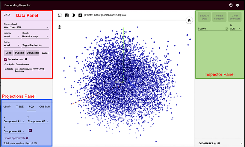
Figure 7.3: Screenshot of the Embedding Projector tool

PCA is a useful tool for visualizing datasets and for finding linear relationships between variables. It can also be used for clustering, outlier detection, and feature selection. Next, we will learn about the k-means algorithm, a method for clustering data.

K-means clustering

K-means clustering, as the name suggests, is a technique to cluster data, that is, to partition data into a specified number of data points. It is an unsupervised learning technique. It works by identifying patterns in the given data. Remember the sorting hat of Harry Potter fame? What it is doing in the book is clustering—dividing new (unlabelled) students into four different clusters: Gryffindor, Ravenclaw, Hufflepuff, and Slytherin.

Humans are very good at grouping objects together; clustering algorithms try to give a similar capability to computers. There are many clustering techniques available, such as hierarchical, Bayesian, or partitional. K-means clustering belongs to partitional clustering; it partitions data into k clusters. Each cluster has a center, called the centroid. The number of clusters k has to be specified by the user.

The k-means algorithm works in the following manner:

1. Randomly choose k data points as the initial centroids (cluster centers).
2. Assign each data point to the closest centroid; there can be different measures to find closeness, the most common being the Euclidean distance.
3. Recompute the centroids using current cluster membership, such that the sum of squared distances decreases.
4. Repeat the last two steps until convergence is met.

In the previous TensorFlow versions, the KMeans class was implemented in the Contrib module; however, the class is no longer available in TensorFlow 2.0. Here we will instead use the advanced mathematical functions provided in TensorFlow 2.0 to implement k-means clustering.

K-means in TensorFlow

To demonstrate k-means in TensorFlow, we will use randomly generated data in the code that follows. Our randomly generated data will contain 200 samples, and we will divide them into three clusters. We start by importing all the required modules, defining the variables, and determining the number of sample points (points_n), the number of clusters to be formed (clusters_n), and the number of iterations we will be doing (iteration_n). We also set the seed for a random number to ensure that our work is reproducible:

import matplotlib.pyplot as plt
import numpy as np
import tensorflow as tf
points_n = 200
clusters_n = 3
iteration_n = 100
seed = 123
np.random.seed(seed)
tf.random.set_seed(seed)

Now we randomly generate data and from the data select three centroids randomly:

points = np.random.uniform(0, 10, (points_n, 2))
centroids = tf.slice(tf.random.shuffle(points), [0, 0], [clusters_n, -1])

Let us now plot the points:

plt.scatter(points[:, 0], points[:, 1], s=50, alpha=0.5)
plt.plot(centroids[:, 0], centroids[:, 1], 'kx', markersize=15)
plt.show()

You can see the scatter plot of all the points and the randomly selected three centroids in the following graph:

Figure 7.4: Randomly generated data, from three randomly selected centroids, plotted

We define the function closest_centroids() to assign each point to the centroid it is closest to:

def closest_centroids(points, centroids):
    distances = tf.reduce_sum(tf.square(tf.subtract(points, centroids[:,None])), 2)
    assignments = tf.argmin(distances, 0)
    return assignments

We create another function move_centroids(). It recalculates the centroids such that the sum of squared distances decreases:

def move_centroids(points, closest, centroids):
    return np.array([points[closest==k].mean(axis=0) for k in range(centroids.shape[0])])

Now we call these two functions iteratively for 100 iterations. We have chosen the number of iterations arbitrarily; you can increase and decrease it to see the effect:

for step in range(iteration_n):
    closest = closest_centroids(points, centroids)
    centroids = move_centroids(points, closest, centroids)

Let us now visualize how the centroids have changed after 100 iterations:

plt.scatter(points[:, 0], points[:, 1], c=closest, s=50, alpha=0.5)
plt.plot(centroids[:, 0], centroids[:, 1], 'kx', markersize=15)
plt.show()

In Figure 7.5, you can see the final centroids after 100 iterations. We have also colored the points based on which centroid they are closest to. The yellow points correspond to one cluster (nearest the cross in its center), and the same is true for the purple and green cluster points:

Figure 7.5: Plot of the final centroids after 100 iterations

In the preceding code, we decided to limit the number of clusters to three, but in most cases with unlabelled data, one is never sure how many clusters exist. One can determine the optimal number of clusters using the elbow method. The method is based on the principle that we should choose the cluster number that reduces the sum of squared error (SSE) distance. If k is the number of clusters, then as k increases, the SSE decreases, with SSE = 0; when k is equal to the number of data points, each point is its own cluster. It is clear we do not want this as our number of clusters, so when we plot the graph between SSE and the number of clusters, we should see a kink in the graph, like the elbow of the hand, which is how the method gets its name – the elbow method. The following code calculates the sum of squared errors for our data:

def sse(points, centroids):
    sse1 = tf.reduce_sum(tf.square(tf.subtract(points, centroids[:,None])), 2).numpy()
    s = np.argmin(sse1, 0)
    distance = 0
    for i in range(len(points)):
      distance += sse1[s[i], i]
    return distance/len(points)

Let us use the elbow method now for finding the optimum number of clusters for our dataset. To do that we will start with one cluster, that is, all points belonging to a single cluster, and increase the number of clusters sequentially. In the code, we increase the clusters by one, with eleven being the maximum number of clusters. For each cluster number value, we use the code above to find the centroids (and hence the clusters) and find the SSE:

w_sse = []
for n in range(1, 11):
  centroids = tf.slice(tf.random.shuffle(points), [0, 0], [n, -1])
  for step in range(iteration_n):
    closest = closest_centroids(points, centroids)
    centroids = move_centroids(points, closest, centroids)
  #print(sse(points, centroids))
  w_sse.append(sse(points, centroids))
plt.plot(range(1, 11),w_sse) 
plt.xlabel('Number of clusters') 

Figure 7.6 shows the different cluster values for the dataset. The kink is clearly visible when the number of clusters is four:

Figure 7.6: Plotting SSE against the number of clusters

K-means clustering is very popular because it is fast, simple, and robust. It also has some disadvantages, the biggest being that the user has to specify the number of clusters. Second, the algorithm does not guarantee global optima; the results can change if the initial randomly chosen centroids change. Third, it is very sensitive to outliers.

Variations in k-means

In the original k-means algorithm each point belongs to a specific cluster (centroid); this is called hard clustering. However, we can have one point belong to all the clusters, with a membership function defining how much it belongs to a particular cluster (centroid). This is called fuzzy clustering or soft clustering.

This variation was proposed in 1973 by J. C. Dunn and later improved upon by J. C. Bezdek in 1981. Though soft clustering takes longer to converge, it can be useful when a point is in multiple classes, or when we want to know how similar a given point is to different clusters.

The accelerated k-means algorithm was created in 2003 by Charles Elkan. He exploited the triangle inequality relationship (that is, a straight line is the shortest distance between two points). Instead of just doing all distance calculations at each iteration, he also kept track of the lower and upper bounds for distances between points and centroids.

In 2006, David Arthur and Sergei Vassilvitskii proposed the k-means++ algorithm. The major change they proposed was in the initialization of centroids. They showed that if we choose centroids that are distant from each other, then the k-means algorithm is less likely to converge on a suboptimal solution.

Another alternative can be that at each iteration we do not use the entire dataset, instead using mini-batches. This modification was proposed by David Sculey in 2010. Now, that we have covered PCA and k-means, we move toward an interesting network called self-organized network or winner-take-all units.

Self-organizing maps

Both k-means and PCA can cluster the input data; however, they do not maintain a topological relationship. In this section, we will consider Self-Organizing Maps (SOMs), sometimes known as Kohonen networks or Winner-Take-All Units (WTUs). They maintain the topological relation. SOMs are a very special kind of neural network, inspired by a distinctive feature of the human brain. In our brain, different sensory inputs are represented in a topologically ordered manner. Unlike other neural networks, neurons are not all connected to each other via weights; instead, they influence each other’s learning. The most important aspect of SOM is that neurons represent the learned inputs in a topographic manner. They were proposed by Teuvo Kohonen [7] in 1982.

In SOMs, neurons are usually placed on the nodes of a (1D or 2D) lattice. Higher dimensions are also possible but are rarely used in practice. Each neuron in the lattice is connected to all the input units via a weight matrix. Figure 7.7 shows a SOM with 6 × 8 (48 neurons) and 5 inputs. For clarity, only the weight vectors connecting all inputs to one neuron are shown. In this case, each neuron will have seven elements, resulting in a combined weight matrix of size 40 × 5:

Figure 7.7: A self-organized map with 5 inputs and 48 neurons

A SOM learns via competitive learning. It can be considered as a nonlinear generalization of PCA and, thus, like PCA, can be employed for dimensionality reduction.

In order to implement SOM, let’s first understand how it works. As a first step, the weights of the network are initialized either to some random value or by taking random samples from the input. Each neuron occupying a space in the lattice will be assigned specific locations. Now as an input is presented, the neuron with the least distance from the input is declared the winner (WTU). This is done by measuring the distance between the weight vectors (W) and input vectors (X) of all neurons:

Here, d_j is the distance of the weights of neuron j from input X. The neuron with the lowest d value is the winner.

Next, the weights of the winning neuron and its neighboring neurons are adjusted in a manner to ensure that the same neuron is the winner if the same input is presented next time.

To decide which neighboring neurons need to be modified, the network uses a neighborhood function ; normally, the Gaussian Mexican hat function is chosen as a neighborhood function. The neighborhood function is mathematically represented as follows:

Here, is a time-dependent radius of the influence of a neuron and d is its distance from the winning neuron. Graphically, the function looks like a hat (hence its name), as you can see in Figure 7.8:

Figure 7.8: The “Gaussian Mexican hat” function, visualized in graph form

Another important property of the neighborhood function is that its radius reduces with time. As a result, in the beginning, many neighboring neurons’ weights are modified, but as the network learns, eventually a few neurons’ weights (at times, only one or none) are modified in the learning process.

The change in weight is given by the following equation:

The process is repeated for all the inputs for a given number of iterations. As the iterations progress, we reduce the learning rate and the radius by a factor dependent on the iteration number.

SOMs are computationally expensive and thus are not really useful for very large datasets. Still, they are easy to understand, and they can very nicely find the similarity between input data. Thus, they have been employed for image segmentation and to determine word similarity maps in NLP.

Colour mapping using a SOM

Some of the interesting properties of the feature map of the input space generated by a SOM are:

• The feature map provides a good representation of the input space. This property can be used to perform vector quantization so that we may have a continuous input space, and using a SOM we can represent it in a discrete output space.
• The feature map is topologically ordered, that is, the spatial location of a neuron in the output lattice corresponds to a particular feature of the input.
• The feature map also reflects the statistical distribution of the input space; the domain that has the largest number of input samples gets a wider area in the feature map.

These features of SOM make them the natural choice for many interesting applications. Here we use SOM for clustering a range of given R, G, and B pixel values to a corresponding color map. We start with the importing of modules:

import tensorflow as tf
import numpy as np
import matplotlib.pyplot as plt

The main component of the code is our class WTU. The class __init__ function initializes various hyperparameters of our SOM, the dimensions of our 2D lattice (m, n), the number of features in the input (dim), the neighborhood radius (sigma), the initial weights, and the topographic information:

# Define the Winner Take All units
class WTU(object):
  #_learned = False
  def __init__(self, m, n, dim, num_iterations, eta = 0.5, sigma = None):
    """
    m x n : The dimension of 2D lattice in which neurons are arranged
    dim : Dimension of input training data
    num_iterations: Total number of training iterations
    eta : Learning rate
    sigma: The radius of neighbourhood function.
    """
    self._m = m
    self._n = n
    self._neighbourhood = []
    self._topography = []
    self._num_iterations = int(num_iterations)
    self._learned = False
    self.dim = dim
    self.eta = float(eta)
    
    if sigma is None:
      sigma = max(m,n)/2.0 # Constant radius
    else:
      sigma = float(sigma)
    self.sigma = sigma
        
    print('Network created with dimensions',m,n)
         
    # Weight Matrix and the topography of neurons
    self._W = tf.random.normal([m*n, dim], seed = 0)
    self._topography = np.array(list(self._neuron_location(m, n)))

The most important function of the class is the training() function, where we use the Kohonen algorithm as discussed before to find the winner units and then update the weights based on the neighborhood function:

def training(self,x, i):
    m = self._m
    n= self._n
    
    # Finding the Winner and its location
    d = tf.sqrt(tf.reduce_sum(tf.pow(self._W - tf.stack([x for i in range(m*n)]),2),1))
    self.WTU_idx = tf.argmin(d,0)
    
    slice_start = tf.pad(tf.reshape(self.WTU_idx, [1]),np.array([[0,1]]))
    self.WTU_loc = tf.reshape(tf.slice(self._topography, slice_start,[1,2]), [2])
    
    
    # Change learning rate and radius as a function of iterations
    learning_rate = 1 - i/self._num_iterations
    _eta_new = self.eta * learning_rate
    _sigma_new = self.sigma * learning_rate
    
    
    # Calculating Neighbourhood function
    distance_square = tf.reduce_sum(tf.pow(tf.subtract(
        self._topography, tf.stack([self.WTU_loc for i in range(m * n)])), 2), 1)
    neighbourhood_func = tf.exp(tf.negative(tf.math.divide(tf.cast(
distance_square, "float32"), tf.pow(_sigma_new, 2))))
    
    # multiply learning rate with neighbourhood func
    eta_into_Gamma = tf.multiply(_eta_new, neighbourhood_func)
    
    # Shape it so that it can be multiplied to calculate dW
    weight_multiplier = tf.stack([tf.tile(tf.slice(
        eta_into_Gamma, np.array([i]), np.array([1])), [self.dim])
        for i in range(m * n)])
    delta_W = tf.multiply(weight_multiplier,
        tf.subtract(tf.stack([x for i in range(m * n)]),self._W))
    new_W = self._W + delta_W
    self._W = new_W

The fit() function is a helper function that calls the training() function and stores the centroid grid for easy retrieval:

def fit(self, X):
    """
    Function to carry out training
    """
    for i in range(self._num_iterations):
        for x in X:
            self.training(x,i)
    # Store a centroid grid for easy retrieval
    centroid_grid = [[] for i in range(self._m)]
    self._Wts = list(self._W)
    self._locations = list(self._topography)
    for i, loc in enumerate(self._locations):
        centroid_grid[loc[0]].append(self._Wts[i])
    self._centroid_grid = centroid_grid
    self._learned = True

Then there are some more helper functions to find the winner and generate a 2D lattice of neurons, and a function to map input vectors to the corresponding neurons in the 2D lattice:

def winner(self, x):
    idx = self.WTU_idx,self.WTU_loc
    return idx
      
def _neuron_location(self,m,n):
    """
    Function to generate the 2D lattice of neurons
    """
    for i in range(m):
       for j in range(n):
          yield np.array([i,j])
def get_centroids(self):
    """
    Function to return a list of 'm' lists, with each inner list containing the 'n' corresponding centroid locations as 1-D NumPy arrays.
    """
    if not self._learned:
       raise ValueError("SOM not trained yet")
    return self._centroid_grid
def map_vects(self, X):
    """
    Function to map each input vector to the relevant neuron in the lattice
    """
    if not self._learned:
       raise ValueError("SOM not trained yet")
       to_return = []
       for vect in X:
          min_index = min([i for i in range(len(self._Wts))],
                           key=lambda x: np.linalg.norm(vect -
                           self._Wts[x]))
          to_return.append(self._locations[min_index])
       return to_return 

We will also need to normalize the input data, so we create a function to do so:

def normalize(df):
    result = df.copy()
    for feature_name in df.columns:
        max_value = df[feature_name].max()
        min_value = df[feature_name].min()
        result[feature_name] = (df[feature_name] - min_value) / (max_value - min_value)
    return result.astype(np.float32)

Let us read the data. The data contains red, green, and blue channel values for different colors. Let us normalize them:

## Reading input data from file
import pandas as pd
df = pd.read_csv('colors.csv')  # The last column of data file is a label
data = normalize(df[['R', 'G', 'B']]).values
name = df['Color-Name'].values
n_dim = len(df.columns) - 1
# Data for Training
colors = data
color_names = name

Let us create our SOM and fit it:

som = WTU(30, 30, n_dim, 400, sigma=10.0)
som.fit(colors)

The fit function takes slightly longer to run, since our code is not optimized for performance but for explaining the concept. Now, let’s look at the result of the trained model. Let us run the following code:

# Get output grid
image_grid = som.get_centroids()
# Map colours to their closest neurons
mapped = som.map_vects(colors)
# Plot
plt.imshow(image_grid)
plt.title('Color Grid SOM')
for i, m in enumerate(mapped):
    plt.text(m[1], m[0], color_names[i], ha='center', va='center',
             bbox=dict(facecolor='white', alpha=0.5, lw=0))

You can see the color map in the 2D neuron lattice:

Figure 7.9: A plotted color map of the 2D neuron lattice

You can see that neurons that win for similar colors are closely placed. Next, we move to an interesting architecture, the restricted Boltzmann machines.

Restricted Boltzmann machines

The RBM is a two-layered neural network—the first layer is called the visible layer and the second layer is called the hidden layer. They are called shallow neural networks because they are only two layers deep. They were first proposed in 1986 by Paul Smolensky (he called them Harmony Networks [1]) and later by Geoffrey Hinton who in 2006 proposed Contrastive Divergence (CD) as a method to train them. All neurons in the visible layer are connected to all the neurons in the hidden layer, but there is a restriction—no neuron in the same layer can be connected. All neurons in the RBM are binary by nature; they will either fire or not fire.

RBMs can be used for dimensionality reduction, feature extraction, and collaborative filtering. The training of RBMs can be divided into three parts: forward pass, backward pass, and then a comparison.

Let us delve deeper into the math. We can divide the operation of RBMs into two passes:

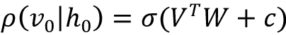
Forward pass: The information at visible units (V) is passed via weights (W) and biases (c) to the hidden units (h₀). The hidden unit may fire or not depending on the stochastic probability ( is the stochastic probability), which is basically the sigmoid function:

Backward pass: The hidden unit representation (h₀) is then passed back to the visible units through the same weights, W, but a different bias, c, where the model reconstructs the input. Again, the input is sampled:

These two passes are repeated for k steps or until the convergence [4] is reached. According to researchers, k=1 gives good results, so we will keep k = 1.

The joint configuration of the visible vector V and the hidden vector h has energy given as follows:

Also associated with each visible vector V is free energy, the energy that a single configuration would need to have in order to have the same probability as all of the configurations that contain V:

Using the contrastive divergence objective function, that is, Mean(F(V_original)) - Mean(F(V_{reconstructed})), the change in weights is given by:

Here, is the learning rate. Similar expressions exist for the biases b and c.

Reconstructing images using an RBM

Let us build an RBM in TensorFlow. The RBM will be designed to reconstruct handwritten digits. This is the first generative model that you are learning; in the upcoming chapters, we will learn a few more. We import the TensorFlow, NumPy, and Matplotlib libraries:

import tensorflow as tf
import numpy as np
import matplotlib.pyplot as plt

We define a class RBM. The class __init_() function initializes the number of neurons in the visible layer (input_size) and the number of neurons in the hidden layer (output_size). The function initializes the weights and biases for both hidden and visible layers. In the following code, we have initialized them to zero. You can try with random initialization as well:

#Class that defines the behavior of the RBM
class RBM(object):
    
    def __init__(self, input_size, output_size, lr=1.0, batchsize=100):
        """
        m: Number of neurons in visible layer
        n: number of neurons in hidden layer
        """
        # Defining the hyperparameters
        self._input_size = input_size # Size of Visible
        self._output_size = output_size # Size of outp
        self.learning_rate = lr # The step used in gradient descent
        self.batchsize = batchsize         # The size of how much data will be used for training per sub iteration
        
        # Initializing weights and biases as matrices full of zeroes
        self.w = tf.zeros([input_size, output_size], np.float32) # Creates and initializes the weights with 0
        self.hb = tf.zeros([output_size], np.float32) # Creates and initializes the hidden biases with 0
        self.vb = tf.zeros([input_size], np.float32) # Creates and initializes the visible biases with 0

We define methods to provide the forward and backward passes:

    # Forward Pass
    def prob_h_given_v(self, visible, w, hb):
        # Sigmoid 
        return tf.nn.sigmoid(tf.matmul(visible, w) + hb)
    # Backward Pass
    def prob_v_given_h(self, hidden, w, vb):
        return tf.nn.sigmoid(tf.matmul(hidden, tf.transpose(w)) + vb)

We create a function to generate random binary values. This is because both hidden and visible units are updated using stochastic probability, depending upon the input to each unit in the case of the hidden layer (and the top-down input to visible layers):

   # Generate the sample probability
    def sample_prob(self, probs):
        return tf.nn.relu(tf.sign(probs - tf.random.uniform(tf.shape(probs))))

We will need functions to reconstruct the input:

def rbm_reconstruct(self,X):
    h = tf.nn.sigmoid(tf.matmul(X, self.w) + self.hb)
    reconstruct = tf.nn.sigmoid(tf.matmul(h, tf.transpose(self.w)) + self.vb)
    return reconstruct

To train the RBM created we define the train() function. The function calculates the positive and negative gradient terms of contrastive divergence and uses the weight update equation to update the weights and biases:

# Training method for the model
def train(self, X, epochs=10):
    
    loss = []
    for epoch in range(epochs):
        #For each step/batch
        for start, end in zip(range(0, len(X), self.batchsize),range(self.batchsize,len(X), self.batchsize)):
            batch = X[start:end]
            
            #Initialize with sample probabilities
            
            h0 = self.sample_prob(self.prob_h_given_v(batch, self.w, self.hb))
            v1 = self.sample_prob(self.prob_v_given_h(h0, self.w, self.vb))
            h1 = self.prob_h_given_v(v1, self.w, self.hb)
            
            #Create the Gradients
            positive_grad = tf.matmul(tf.transpose(batch), h0)
            negative_grad = tf.matmul(tf.transpose(v1), h1)
            
            #Update learning rates 
            self.w = self.w + self.learning_rate *(positive_grad - negative_grad) / tf.dtypes.cast(tf.shape(batch)[0],tf.float32)
            self.vb = self.vb +  self.learning_rate * tf.reduce_mean(batch - v1, 0)
            self.hb = self.hb +  self.learning_rate * tf.reduce_mean(h0 - h1, 0)
            
        #Find the error rate
        err = tf.reduce_mean(tf.square(batch - v1))
        print ('Epoch: %d' % epoch,'reconstruction error: %f' % err)
        loss.append(err)
        
    return loss

Now that our class is ready, we instantiate an object of RBM and train it on the MNIST dataset:

(train_data, _), (test_data, _) =  tf.keras.datasets.mnist.load_data()
train_data = train_data/np.float32(255)
train_data = np.reshape(train_data, (train_data.shape[0], 784))
test_data = test_data/np.float32(255)
test_data = np.reshape(test_data, (test_data.shape[0], 784))
#Size of inputs is the number of inputs in the training set
input_size = train_data.shape[1]
rbm = RBM(input_size, 200)
err = rbm.train(train_data,50)

Let us plot the learning curve:

plt.plot(err)
plt.xlabel('epochs')
plt.ylabel('cost')

In the figure below, you can see the learning curve of our RBM:

Figure 7.10: Learning curve for the RBM model

Now, we present the code to visualize the reconstructed images:

out = rbm.rbm_reconstruct(test_data)
# Plotting original and reconstructed images
row, col = 2, 8
idx = np.random.randint(0, 100, row * col // 2)
f, axarr = plt.subplots(row, col, sharex=True, sharey=True, figsize=(20,4))
for fig, row in zip([test_data,out], axarr):
    for i,ax in zip(idx,row):
        ax.imshow(tf.reshape(fig[i],[28, 28]), cmap='Greys_r')
        ax.get_xaxis().set_visible(False)
        ax.get_yaxis().set_visible(False)

And the reconstructed images:

Figure 7.11: Image reconstruction using an RBM

The top row is the input handwritten image, and the bottom row is the reconstructed image. You can see that the images look remarkably similar to the human handwritten digits. In the upcoming chapters, you will learn about models that can generate even more complex images such as artificial human faces.

Deep belief networks

Now that we have a good understanding of RBMs and know how to train them using contrastive divergence, we can move toward the first successful deep neural network architecture, the deep belief networks (DBNs), proposed in 2006 by Hinton and his team in the paper A fast learning algorithm for deep belief nets. Before this model it was very difficult to train deep architectures, not just because of the limited computing resources, but also, as will be discussed in Chapter 8, Autoencoders, because of the vanishing gradient problem. In DBNs it was first demonstrated how deep architectures can be trained via greedy layer-wise training.

In the simplest terms, DBNs are just stacked RBMs. Each RBM is trained separately using the contrastive divergence. We start with the training of the first RBM layer. Once it is trained, we train the second RBM layer. The visible units of the second RBM are now fed the output of the hidden units of the first RBM, when it is fed the input data. The procedure is repeated with each RBM layer addition.

Let us try stacking our RBM class. To make the DBN, we will need to define one more function in the RBM class; the output of the hidden unit of one RBM needs to feed into the next RBM:

    #Create expected output for our DBN
    def rbm_output(self, X):
        out = tf.nn.sigmoid(tf.matmul(X, self.w) + self.hb)
        return out

Now we can just use the RBM class to create a stacked RBM structure. In the following code we create an RBM stack: the first RBM will have 500 hidden units, the second will have 200 hidden units, and the third will have 50 hidden units:

RBM_hidden_sizes = [500, 200 , 50 ] #create 2 layers of RBM with size 400 and 100
#Since we are training, set input as training data
inpX = train_data
#Create list to hold our RBMs
rbm_list = []
#Size of inputs is the number of inputs in the training set
input_size = train_data.shape[1]
#For each RBM we want to generate
for i, size in enumerate(RBM_hidden_sizes):
    print ('RBM: ',i,' ',input_size,'->', size)
    rbm_list.append(RBM(input_size, size))
    input_size = size

---------------------------------------------------------------------
RBM:  0   784 -> 500
RBM:  1   500 -> 200
RBM:  2   200 -> 50

For the first RBM, the MNIST data is the input. The output of the first RBM is then fed as input to the second RBM, and so on through the consecutive RBM layers:

#For each RBM in our list
for rbm in rbm_list:
    print ('Next RBM:')
    #Train a new one
    rbm.train(tf.cast(inpX,tf.float32))
    #Return the output layer
    inpX = rbm.rbm_output(inpX)

Our DBN is ready. The three stacked RBMs are now trained using unsupervised learning. DBNs can also be trained using supervised training. To do so we need to fine-tune the weights of the trained RBMs and add a fully connected layer at the end. In their publication Classification with Deep Belief Networks, Hebbo and Kim show how they used a DBN for MNIST classification; it is a good introduction to the subject.

Summary

In this chapter, we covered the major unsupervised learning algorithms. We went through algorithms best suited for dimension reduction, clustering, and image reconstruction. We started with the dimension reduction algorithm PCA, then we performed clustering using k-means and self-organized maps. After this we studied the restricted Boltzmann machine and saw how we can use it for both dimension reduction and image reconstruction. Next, we delved into stacked RBMs, that is, deep belief networks, and we trained a DBN consisting of three RBM layers on the MNIST dataset.

In the next chapter, we will explore another model using an unsupervised learning paradigm – autoencoders.

References

1. Smith, Lindsay. (2006). A tutorial on Principal Component Analysis: http://www.cs.otago.ac.nz/cosc453/student_tutorials/principal_components.pdf
2. Movellan, J. R. Tutorial on Principal component Analysis: http://mplab.ucsd.edu/tutorials/pca.pdf
3. TensorFlow Projector: http://projector.tensorflow.org/
4. Singular Value Decomposition (SVD) tutorial. MIT: https://web.mit.edu/be.400/www/SVD/Singular_Value_Decomposition.htm
5. Shlens, Jonathon. (2014). A tutorial on principal component analysis. arXiv preprint arXiv:1404.1100: https://arxiv.org/abs/1404.1100
6. Goodfellow, I., Bengio, Y., and Courville, A. (2016). Deep learning. MIT press: https://www.deeplearningbook.org
7. Kohonen, T. (1982). Self-organized formation of topologically correct feature maps. Biological cybernetics 43, no. 1: 59-69.
8. Kanungo, Tapas, et al. (2002). An Efficient k-Means Clustering Algorithm: Analysis and Implementation. IEEE transactions on pattern analysis and machine intelligence 24.7: 881-892.
9. Ortega, Joaquín Pérez, et al. Research issues on K-means Algorithm: An Experimental Trial Using Matlab. CEUR Workshop Proceedings: Semantic Web and New Technologies.
10. Chen, K. (2009). On Coresets for k-Median and k-Means Clustering in Metric and Euclidean Spaces and Their Applications. SIAM Journal on Computing 39.3: 923-947.
11. Determining the number of clusters in a data set: https://en.wikipedia.org/wiki/Determining_the_number_of_clusters_in_a_data_set
12. Lloyd, S. P. (1982). Least Squares Quantization in PCM: http://mlsp.cs.cmu.edu/courses/fall2010/class14/lloyd.pdf
13. Dunn, J. C. (1973-01-01). A Fuzzy Relative of the ISODATA Process and Its Use in Detecting Compact Well-Separated Clusters. Journal of Cybernetics. 3(3): 32–57.
14. Bezdek, James C. (1981). Pattern Recognition with Fuzzy Objective Function Algorithms.
15. Peters, G., Crespo, F., Lingras, P., and Weber, R. (2013). Soft clustering–Fuzzy and rough approaches and their extensions and derivatives. International Journal of Approximate Reasoning 54, no. 2: 307-322.
16. Sculley, D. (2010). Web-scale k-means clustering. In Proceedings of the 19th international conference on World wide web, pp. 1177-1178. ACM.
17. Smolensky, P. (1986). Information Processing in Dynamical Systems: Foundations of Harmony Theory. No. CU-CS-321-86. COLORADO UNIV AT BOULDER DEPT OF COMPUTER SCIENCE.
18. Salakhutdinov, R., Mnih, A., and Hinton, G. (2007). Restricted Boltzmann Machines for Collaborative Filtering. Proceedings of the 24th international conference on Machine learning. ACM.
19. Hinton, G. (2010). A Practical Guide to Training Restricted Boltzmann Machines. Momentum 9.1: 926.

Join our book’s Discord space

Join our Discord community to meet like-minded people and learn alongside more than 2000 members at: https://packt.link/keras