12

Probabilistic TensorFlow

Uncertainty is a fact of life; whether you are doing a classification task or a regression task, it is important to know how confident your model is in its prediction. Till now, we have covered the traditional deep learning models, and while they are great at many tasks, they are not able to handle uncertainty. Instead, they are deterministic in nature. In this chapter, you will learn how to leverage TensorFlow Probability to build models that can handle uncertainty, specifically probabilistic deep learning models and Bayesian networks. The chapter will include:

• TensorFlow Probability
• Distributions, events, and shapes in TensorFlow Probability
• Bayesian networks using TensorFlow Probability
• Understand uncertainty in machine learning models
• Model aleatory and epistemic uncertainty using TensorFlow Probability

Let’s start with first understanding TensorFlow Probability.

TensorFlow Probability

TensorFlow Probability (TFP), a part of the TensorFlow ecosystem, is a library that provides tools for developing probabilistic models. It can be used to perform probabilistic reasoning and statistical analysis. It is built over TensorFlow and provides the same computational advantage.

Figure 12.1 shows the major components constituting TensorFlow Probability:

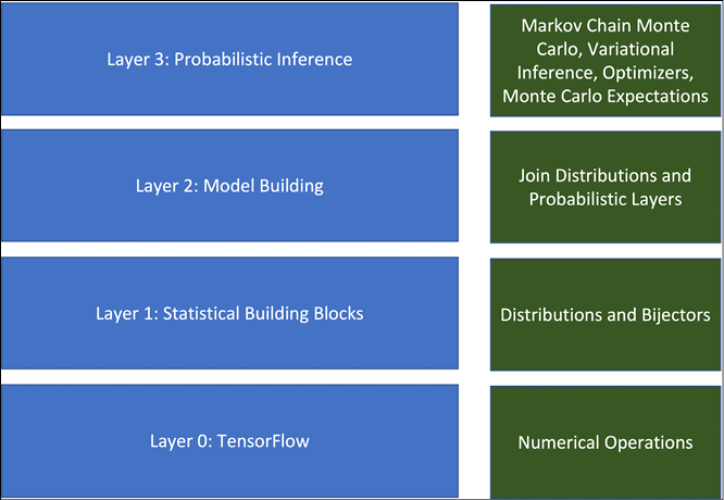
Figure 12.1: Different components of TensorFlow Probability

At the root, we have all numerical operations supported by TensorFlow, specifically the LinearOperator class (part of tf.linalg) – it contains all the methods that can be performed on a matrix, without the need to actually materialize the matrix. This provides computationally efficient matrix-free computations. TFP includes a large collection of probability distributions and their related statistical computations. It also has tfp.bijectors, which offers a wide range of transformed distributions.

TensorFlow Probability also provides JointDistribution, which allows the user to draw a joint sample and compute a joint log-density (log probability density function). The standard TFP distributions work on tensors, but JointDistribution works on the structure of tensors. tfp.layers provides neural network layers that can be used to extend the standard TensorFlow layers and add uncertainty to them. And finally, it provides a wide range of tools for probabilistic inference. In this chapter, we will go through some of these functions and classes; let us first start with installation. To install TFP in your working environment, just run:

pip install tensorflow-probability

Let us have some fun with TFP. To use TFP, we will need to import it. Additionally, we are going to do some plots. So, we import some additional modules:

import matplotlib.pyplot as plt
import tensorflow_probability as tfp
import functools, inspect, sys

Next, we explore the different classes of distributions available in tfp.distributions:

tfd = tfp.distributions
distribution_class =  tfp.distributions.Distribution
distributions = [name for name, obj in inspect.getmembers(tfd)
                if inspect.isclass(obj) and issubclass(obj, distribution_class)]
print(distributions)

Here is the output:

['Autoregressive', 'BatchBroadcast', 'BatchConcat', 'BatchReshape', 'Bates', 'Bernoulli', 'Beta', 'BetaBinomial', 'BetaQuotient', 'Binomial', 'Blockwise', 'Categorical', 'Cauchy', 'Chi', 'Chi2', 'CholeskyLKJ', 'ContinuousBernoulli', 'DeterminantalPointProcess', 'Deterministic', 'Dirichlet', 'DirichletMultinomial', 'Distribution', 'DoublesidedMaxwell', 'Empirical', 'ExpGamma', 'ExpInverseGamma', 'ExpRelaxedOneHotCategorical', 'Exponential', 'ExponentiallyModifiedGaussian', 'FiniteDiscrete', 'Gamma', 'GammaGamma', 'GaussianProcess', 'GaussianProcessRegressionModel', 'GeneralizedExtremeValue', 'GeneralizedNormal', 'GeneralizedPareto', 'Geometric', 'Gumbel', 'HalfCauchy', 'HalfNormal', 'HalfStudentT', 'HiddenMarkovModel', 'Horseshoe', 'Independent', 'InverseGamma', 'InverseGaussian', 'JohnsonSU', 'JointDistribution', 'JointDistributionCoroutine', 'JointDistributionCoroutineAutoBatched', 'JointDistributionNamed', 'JointDistributionNamedAutoBatched', 'JointDistributionSequential', 'JointDistributionSequentialAutoBatched', 'Kumaraswamy', 'LKJ', 'LambertWDistribution', 'LambertWNormal', 'Laplace', 'LinearGaussianStateSpaceModel', 'LogLogistic', 'LogNormal', 'Logistic', 'LogitNormal', 'MarkovChain', 'Masked', 'MatrixNormalLinearOperator', 'MatrixTLinearOperator', 'Mixture', 'MixtureSameFamily', 'Moyal', 'Multinomial', 'MultivariateNormalDiag', 'MultivariateNormalDiagPlusLowRank', 'MultivariateNormalDiagPlusLowRankCovariance', 'MultivariateNormalFullCovariance', 'MultivariateNormalLinearOperator', 'MultivariateNormalTriL', 'MultivariateStudentTLinearOperator', 'NegativeBinomial', 'Normal', 'NormalInverseGaussian', 'OneHotCategorical', 'OrderedLogistic', 'PERT', 'Pareto', 'PixelCNN', 'PlackettLuce', 'Poisson', 'PoissonLogNormalQuadratureCompound', 'PowerSpherical', 'ProbitBernoulli', 'QuantizedDistribution', 'RelaxedBernoulli', 'RelaxedOneHotCategorical', 'Sample', 'SigmoidBeta', 'SinhArcsinh', 'Skellam', 'SphericalUniform', 'StoppingRatioLogistic', 'StudentT', 'StudentTProcess', 'StudentTProcessRegressionModel', 'TransformedDistribution', 'Triangular', 'TruncatedCauchy', 'TruncatedNormal', 'Uniform', 'VariationalGaussianProcess', 'VectorDeterministic', 'VonMises', 'VonMisesFisher', 'Weibull', 'WishartLinearOperator', 'WishartTriL', 'Zipf']

You can see that a rich range of distributions is available in TFP. Let us now try one of the distributions:

normal = tfd.Normal(loc=0., scale=1.)

This statement declares that we want to have a normal distribution with mean (loc) zero and standard deviation (scale) 1. We can generate random samples following this distribution using the sample method. The following code snippet generates such N samples and plots them:

def plot_normal(N):
  samples = normal.sample(N)
  sns.distplot(samples)
  plt.title(f"Normal Distribution with zero mean, and 1 std. dev {N} samples")
  plt.show()

You can see that as N increases, the plot follows a nice normal distribution:

Figure 12.2: Normal distribution from randomly generated samples of sizes 100, 1,000, and 10,000. The distribution has a mean of zero and a standard deviation of one

Let us now explore the different distributions available with TFP.

TensorFlow Probability distributions

Every distribution in TFP has a shape, batch, and event size associated with it. The shape is the sample size; it represents independent and identically distributed draws or observations. Consider the normal distribution that we defined in the previous section:

normal = tfd.Normal(loc=0., scale=1.)

This defines a single normal distribution, with mean zero and standard deviation one. When we use the sample function, we do a random draw from this distribution.

Notice the details regarding batch_shape and event_shape if you print the object normal:

print(normal)

>>> tfp.distributions.Normal("Normal", batch_shape=[], event_shape=[], dtype=float32)

Let us try and define a second normal object, but this time, loc and scale are lists:

normal_2 = tfd.Normal(loc=[0., 0.], scale=[1., 3.])
print(normal_2)

>>> tfp.distributions.Normal("Normal", batch_shape=[2], event_shape=[], dtype=float32)

Did you notice the change in batch_shape? Now, if we draw a single sample from it, we will draw from two normal distributions, one with a mean of zero and standard deviation of one, and the other with a mean of zero and standard deviation of three. Thus, the batch shape determines the number of observations from the same distribution family. The two normal distributions are independent; thus, it is a batch of distributions of the same family.

What if we need a single normal distribution that is dependent on two variables, each with a different mean? This is made possible using MultivariateNormalDiag, and this influences the event shape – it is the atomic shape of a single draw or observation from this distribution:

normal_3 = tfd.MultivariateNormalDiag(loc = [[1.0, 0.3]])
print(normal_3)

>>> tfp.distributions.MultivariateNormalDiag("MultivariateNormalDiag", batch_shape=[1], event_shape=[2], dtype=float32)

We can see that in the above output the event_shape has changed.

Using TFP distributions

Once you have defined a distribution, you can do a lot more. TFP provides a good range of functions to perform various operations. We have already used the Normal distribution and sample method. The section above also demonstrated how we can use TFP for creating univariate, multivariate, or independent distribution/s. TFP provides many important methods to interact with the created distributions. Some of the important ones include:

• sample(n): It samples n observations from the distribution.
• prob(value): It provides probability (discrete) or probability density (continuous) for the value.
• log_prob(values): Provides log probability or log-likelihood for the values.
• mean(): It gives the mean of the distribution.
• stddev(): It provides the standard deviation of the distribution.

Coin Flip Example

Let us now use some of the features of TFP to describe data by looking at an example: the standard coin-flipping example we are familiar with from our school days. We know that if we flip a coin, there are only two possibilities – we can have either a head or a tail. Such a distribution, where we have only two discrete values, is called a Bernoulli distribution. So let us consider different scenarios:

Scenario 1

A fair coin with a 0.5 probability of heads and 0.5 probability of tails.

Let us create the distribution:

coin_flip = tfd.Bernoulli(probs=0.5, dtype=tf.int32)

Now get some samples:

coin_flip_data = coin_flip.sample(2000)

Let us visualize the samples:

plt.hist(coin_flip_data)

Figure 12.3: Distribution of heads and tails from 2,000 observations

You can see that we have both heads and tails in equal numbers; after all, it is a fair coin. The probability of heads and tails as 0.5:

coin_flip.prob(0) ## Probability of tail

>>> <tf.Tensor: shape=(), dtype=float32, numpy=0.5>

Scenario 2

A biased coin with a 0.8 probability of heads and 0.2 probability of tails.

Now, since the coin is biased, with the probability of heads being 0.8, the distribution would be created using:

bias_coin_flip = tfd.Bernoulli(probs=0.8, dtype=tf.int32)

Now get some samples:

bias_coin_flip_data = bias_coin_flip.sample(2000)

Let us visualize the samples:

plt.hist(bias_coin_flip_data)

Figure 12.4: Distribution of heads and tails from 2,000 coin flips of a biased coin

We can see that now heads are much larger in number than tails. Thus, the probability of tails is no longer 0.5:

bias_coin_flip.prob(0) ## Probability of tail

>>> <tf.Tensor: shape=(), dtype=float32, numpy=0.19999999>

You will probably get a number close to 0.2.

Scenario 3

Two coins with one biased toward heads with a 0.8 probability, and the other biased toward heads with a 0.6 probability.

Now, we have two independent coins. Since the coins are biased, with the probabilities of heads being 0.8 and 0.6 respectively, we create a distribution using:

two_bias_coins_flip = tfd.Bernoulli(probs=[0.8, 0.6], dtype=tf.int32)

Now get some samples:

two_bias_coins_flip_data = two_bias_coins_flip.sample(2000)

Let us visualize the samples:

plt.hist(two_bias_coins_flip_data[:,0], alpha=0.8, label='Coin 1')
plt.hist(two_bias_coins_flip_data[:,1], alpha=0.5, label='Coin 2')
plt.legend(loc='center')

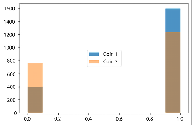
Figure 12.5: Distribution of heads and tails from 2,000 flips for two independent coins

The bar in blue corresponds to Coin 1, and the bar in orange corresponds to Coin 2. The brown part of the graphs is the area where the results of the two coins overlap. You can see that for Coin 1, the number of heads is much larger as compared to Coin 2, as expected.

Normal distribution

We can use the Bernoulli distribution where the data can have only two possible discrete values: heads and tails, good and bad, spam and ham, and so on. However, a large amount of data in our daily lives is continuous in range, with the normal distribution being very common. So let us also explore different normal distributions.

Mathematically, the probability density function of a normal distribution can be expressed as:

where is the mean of the distribution, and is the standard deviation.

In TFP, the parameter loc represents the mean and the parameter scale represents the standard deviation. Now, to illustrate the use of how we can use distribution, let us consider that we want to represent the weather data of a location for a particular season, say summer in Delhi, India.

Univariate normal

We can think that weather depends only on temperature. So, by having a sample of temperature in the summer months over many years, we can get a good representation of data. That is, we can have a univariate normal distribution.

Now, based on weather data, the average high temperature in the month of June in Delhi is 35 degrees Celsius, with a standard deviation of 4 degrees Celsius. So, we can create a normal distribution using:

temperature = tfd.Normal(loc=35, scale = 4)

Get some observation samples from it:

temperature_data = temperature.sample(1000)

And let us now visualize it:

sns.displot(temperature_data, kde= True)

Figure 12.6: Probability density function for the temperature of Delhi in the month of June

It would be good to verify if the mean and standard deviation of our sample data is close to the values we described.

Using the distribution, we can find the mean and standard deviation using:

temperature.mean()

# output
>>> <tf.Tensor: shape=(), dtype=float32, numpy=35.0>

temperature.stddev()

# output
>>> <tf.Tensor: shape=(), dtype=float32, numpy=4.0>

And from the sampled data, we can verify using:

tf.math.reduce_mean(temperature_data) 

# output
>>> <tf.Tensor: shape=(), dtype=float32, numpy=35.00873>

tf.math.reduce_std(temperature_data)

# output
>>> <tf.Tensor: shape=(), dtype=float32, numpy=3.9290223>

Thus, the sampled data is following the same mean and standard deviation.

Multivariate distribution

All is good so far. I show my distribution to a friend working in meteorology, and he says that using only temperature is not sufficient; the humidity is also important. So now, each weather point depends on two parameters – the temperature of the day and the humidity of the day. This type of data distribution can be obtained using the MultivariateNormalDiag distribution class, as defined in TFP:

weather = tfd.MultivariateNormalDiag(loc = [35, 56], scale_diag=[4, 15])
weather_data = weather.sample(1000)
plt.scatter(weather_data[:, 0], weather_data[:, 1], color='blue', alpha=0.4)
plt.xlabel("Temperature Degree Celsius")
plt.ylabel("Humidity %")

Figure 12.7, shows the multivariate normal distribution of two variables, temperature and humidity, generated using TFP:

Figure 12.7: Multivariate normal distribution with the x-axis representing temperature and the y-axis humidity

Using the different distributions and bijectors available in TFP, we can generate synthetic data that follows the same joint distribution as real data to train the model.

Bayesian networks

Bayesian Networks (BNs) make use of the concepts from graph theory, probability, and statistics to encapsulate complex causal relationships. Here, we build a Directed Acyclic Graph (DAG), where nodes, called factors (random variables), are connected by the arrows representing cause-effect relationships. Each node represents a variable with an associated probability (also called a Conditional Probability Table (CPT)). The links tell us about the dependence of one node over another. Though they were first proposed by Pearl in 1988, they have regained attention in recent years. The main cause of this renowned interest in BNs is that standard deep learning models are not able to represent the cause-effect relationship.

Their strength lies in the fact that they can be used to model uncertainties combined with expert knowledge and data. They have been employed in diverse fields for their power to do probabilistic and causal reasoning. At the heart of the Bayesian network is Bayes’ rule:

Bayes’ rule is used to determine the joint probability of an event given certain conditions. The simplest way to understand the BN is that the BN can determine the causal relationship between the hypothesis and evidence. There is some unknown hypothesis H, about which we want to assess the uncertainty and make some decisions. We start with some prior belief about hypothesis H, and then based on evidence E, we update our belief about H.

Let us try to understand it by example. We consider a very standard example: a garden with grass and a sprinkler. Now, using common sense, we know that if the sprinkler is on, the grass is wet. Let us now reverse the logic: what if you come back home and find that the grass is wet, what is the probability that the sprinkler is on, and what is the probability that it actually rained? Interesting, right? Let us add further evidence – you find that the sky is cloudy. Now, what do you think is the reason for the grass being wet?

This sort of reasoning based on evidence is encompassed by BNs in the form of DAGs, also called causal graphs – because they provide an insight into the cause-effect relationship.

To model the problem, we make use of the JointDistributionCoroutine distribution class. This distribution allows both the sampling of data and computation of the joint probability from a single model specification. Let us make some assumptions to build the model:

• The probability that it is cloudy is 0.2
• The probability that it is cloudy and it rains is 0.8, and the probability that it is not cloudy but it rains is 0.1
• The probability that it is cloudy and the sprinkler is on is 0.1, and the probability that it is not cloudy and the sprinkler is on is 0.5
• Now, for the grass, we have four possibilities:

Table 12.1: The conditional probability table for the Sprinkler-Rain-Grass scenario

Figure 12.8 shows the corresponding BN DAG:

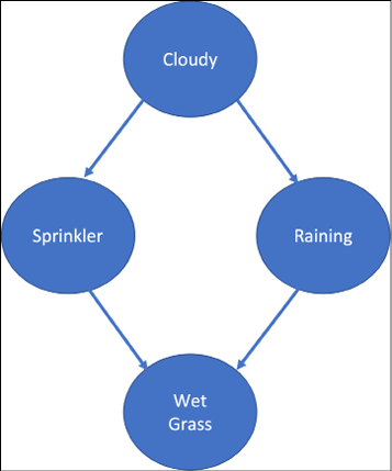
Figure 12.8: Bayesian Network for our toy problem

This information can be represented by the following model:

Root = tfd.JointDistributionCoroutine.Root
def model():
  # generate the distribution for cloudy weather
  cloudy = yield Root(tfd.Bernoulli(probs=0.2, dtype=tf.int32))
  # define sprinkler probability table
  sprinkler_prob = [0.5, 0.1]
  sprinkler_prob = tf.gather(sprinkler_prob, cloudy)
  sprinkler = yield tfd.Bernoulli(probs=sprinkler_prob, dtype=tf.int32)
  # define rain probability table
  raining_prob = [0.1, 0.8]
  raining_prob = tf.gather(raining_prob, cloudy)
  raining = yield tfd.Bernoulli(probs=raining_prob, dtype=tf.int32)
  #Conditional Probability table for wet grass
  grass_wet_prob = [[0.0, 0.8],
                    [0.9, 0.99]]
  grass_wet_prob = tf.gather_nd(grass_wet_prob, _stack(sprinkler, raining))
  grass_wet = yield tfd.Bernoulli(probs=grass_wet_prob, dtype=tf.int32)

The above model will function like a data generator. The Root function is used to tell the node in the graph without any parent. We define a few utility functions, broadcast and stack:

def _conform(ts):
  """Broadcast all arguments to a common shape."""
  shape = functools.reduce(
      tf.broadcast_static_shape, [a.shape for a in ts])
  return [tf.broadcast_to(a, shape) for a in ts]
def _stack(*ts):
  return tf.stack(_conform(ts), axis=-1)

To do inferences, we make use of the MarginalizableJointDistributionCoroutine class, as this allows us to compute marginalized probabilities:

d = marginalize.MarginalizableJointDistributionCoroutine(model)

Now, based on our observations, we can obtain the probability of other factors.

Case 1:

We observe that the grass is wet (the observation corresponding to this is 1 – if the grass was dry, we would set it to 0), we have no idea about the state of the clouds or the state of the sprinkler (the observation corresponding to an unknown state is set to “marginalize”), and we want to know the probability of rain (the observation corresponding to the probability we want to find is set to “tabulate”). Converting this into observations:

observations = ['marginalize', # We don't know the cloudy state
                'tabulate', # We want to know the probability of rain
                'marginalize', # We don't know the sprinkler state.
                1]             # We observed a wet lawn.

Now we get the probability of rain using:

p = tf.exp(d.marginalized_log_prob(observations))
p = p / tf.reduce_sum(p)

The result is array([0.27761015, 0.72238994], dtype=float32), that is, there is a 0.722 probability that it rained.

Case 2:

We observe that the grass is wet, we have no idea about the state of the clouds or rain, and we want to know the probability of whether the sprinkler is on. Converting this into observations:

observations = ['marginalize',  
                'marginalize', 
                'tabulate',  
                1]

This results in probabilities array([0.61783344, 0.38216656], dtype=float32), that is, there is a 0.382 probability that the sprinkler is on.

Case 3:

What if we observe that there is no rain, and the sprinkler is off? What do you think is the state of the grass? Logic says the grass should not be wet. Let us confirm this from the model by sending it the observations:

observations = ['marginalize',  
                 0,
                 0, 
                'tabulate']

This results in the probabilities array([1., 0], dtype=float32), that is, there is a 100% probability that the grass is dry, just the way we expected.

As you can see, once we know the state of the parents, we do not need to know the state of the parent’s parents – that is, the BN follows the local Markov property. In the example that we covered here, we started with the structure, and we had the conditional probabilities available to us. We demonstrate how we can do inference based on the model, and how despite the same model and CPDs, the evidence changes the posterior probabilities.

Handling uncertainty in predictions using TensorFlow Probability

At the beginning of this chapter, we talked about the uncertainties in prediction by deep learning models and how the existing deep learning architectures are not able to account for those uncertainties. In this chapter, we will use the layers provided by TFP to model uncertainty.

Before adding the TFP layers, let us first understand the uncertainties a bit. There are two classes of uncertainty.

Aleatory uncertainty

This exists because of the random nature of the natural processes. It is inherent uncertainty, present due to the probabilistic variability. For example, when tossing a coin, there will always be a certain degree of uncertainty in predicting whether the next toss will be heads or tails. There is no way to remove this uncertainty. In essence, every time you repeat the experiment, the results will have certain variations.

Epistemic uncertainty

This uncertainty comes from a lack of knowledge. There can be various reasons for this lack of knowledge, for example, an inadequate understanding of the underlying processes, an incomplete knowledge of the phenomena, and so on. This type of uncertainty can be reduced by understanding the reason, for example, to get more data, we conduct more experiments.

The presence of these uncertainties increases risk. We require a way to quantify these uncertainties and, hence, quantify the risk.

Creating a synthetic dataset

In this section, we will learn how to modify the standard deep neural networks to quantify uncertainties. Let us start with creating a synthetic dataset. To create the dataset, we consider that output prediction y depends on input x linearly, as given by the following expression:

Here, follows a normal distribution with mean zero and standard deviation 1 around x. The function below will generate this synthetic data for us. Do observe that to generate this data, we made use of the Uniform distribution and Normal distributions available as part of TFP distributions:

def create_dataset(n, x_range):
    x_uniform_dist = tfd.Uniform(low=x_range[0], high=x_range[1])
    x = x_uniform_dist.sample(n).numpy() [:, np.newaxis] 
    y_true = 2.7*x+3
    eps_uniform_dist = tfd.Normal(loc=0, scale=1)
    eps = eps_uniform_dist.sample(n).numpy() [:, np.newaxis] *0.74*x
    y = y_true + eps
    return x, y, y_true

y_true is the value without including the normal distributed noise .

Now we use it to create a training dataset and a validation dataset:

x_train, y_train, y_true = create_dataset(2000, [-10, 10])
x_val, y_val, _ = create_dataset(500, [-10, 10])

This will give us 2,000 datapoints for training and 500 datapoints for validation. Figure 12.9 shows the plots of the two datasets, with ground truth (the value of y in the absence of any noise) in the background:

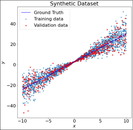
Figure 12.9: Plot of the synthetic dataset

Building a regression model using TensorFlow

We can build a simple Keras model to perform the task of regression on the synthetic dataset created in the preceding section:

# Model Architecture
model = Sequential([Dense(1, input_shape=(1,))])
# Compile 
model.compile(loss='mse', optimizer='adam')
# Fit
model.fit(x_train, y_train, epochs=100, verbose=1)

Let us see how good the fitted model works on the test dataset:

Figure 12.10: Ground truth and fitted regression line

It was a simple problem, and we can see that the fitted regression line almost overlaps the ground truth. However, there is no way to tell the uncertainty of predictions.

Probabilistic neural networks for aleatory uncertainty

What if instead of linear regression, we build a model that can fit the distribution? In our synthetic dataset, the source of aleatory uncertainty is the noise, and we know that our noise follows a normal distribution, which is characterized by two parameters: the mean and standard deviation. So, we can modify our model to predict the mean and standard deviation distributions instead of actual y values. We can accomplish this using either the IndependentNormal TFP layer or the DistributionLambda TFP layer. The following code defines the modified model architecture:

model = Sequential([Dense(2, input_shape = (1,)),
    tfp.layers.DistributionLambda(lambda t: tfd.Normal(loc=t[..., :1], scale=0.3+tf.math.abs(t[...,1:])))
])

We will need to make one more change. Earlier, we predicted the y value; therefore, the mean square error loss was a good choice. Now, we are predicting the distribution; therefore, a better choice is the negative log-likelihood as the loss function:

# Define negative loglikelihood loss function
def neg_loglik(y_true, y_pred):
    return -y_pred.log_prob(y_true)

Let us now train this new model:

model.compile(loss=neg_loglik, optimizer='adam')
# Fit
model.fit(x_train, y_train, epochs=500, verbose=1)

Since now our model returns a distribution, we require the statistics mean and standard deviation for the test dataset:

# Summary Statistics
y_mean = model(x_test).mean()
y_std = model(x_test).stddev()

Note that the predicted mean now corresponds to the fitted line in the first case. Let us now see the plots:

fig = plt.figure(figsize = (20, 10))
plt.scatter(x_train, y_train, marker='+', label='Training Data', alpha=0.5)
plt.plot(x_train, y_true, color='k', label='Ground Truth')
plt.plot(x_test, y_mean, color='r', label='Predicted Mean')
plt.fill_between(np.squeeze(x_test), np.squeeze(y_mean+1*y_std), np.squeeze(y_mean-1*y_std),  alpha=0.6, label='Aleatory Uncertainty (1SD)')
plt.fill_between(np.squeeze(x_test), np.squeeze(y_mean+2*y_std), np.squeeze(y_mean-2*y_std),  alpha=0.4, label='Aleatory Uncertainty (2SD)')
plt.title('Aleatory Uncertainty')
plt.xlabel('$x$')
plt.ylabel('$y$')
plt.legend()
plt.show()

The following curve shows the fitted line, along with the aleatory uncertainty:

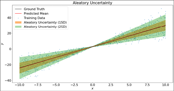
Figure 12.11: Modelling aleatory uncertainty using TFP layers

You can see that our model shows less uncertainty near the origin, but as we move further away, the uncertainty increases.

Accounting for the epistemic uncertainty

In conventional neural networks, each weight is represented by a single number, and it is updated such that the loss of the model with respect to its weight is minimized. We assume that weights so learned are the optimum weights. But are they? To answer this question, we replace each weight with a distribution, and instead of learning a single value, we will now make our model learn a set of parameters for each weight distribution. This is accomplished by replacing the Keras Dense layer with the DenseVariational layer. The DenseVariational layer uses a variational posterior over the weights to represent the uncertainty in their values. It tries to regularize the posterior to be close to the prior distribution. Hence, to use the DenseVariational layer, we will need to define two functions, one prior generating function and another posterior generating function. We use the posterior and prior functions defined at https://www.tensorflow.org/probability/examples/Probabilistic_Layers_Regression.

Our model now has two layers, a DenseVariational layer followed by a DistributionLambda layer:

model = Sequential([
  tfp.layers.DenseVariational(1, posterior_mean_field, prior_trainable, kl_weight=1/x_train.shape[0]),
  tfp.layers.DistributionLambda(lambda t: tfd.Normal(loc=t, scale=1)),
])

Again, as we are looking for distributions, the loss function that we use is the negative log-likelihood function:

model.compile(optimizer=tf.optimizers.Adam(learning_rate=0.01), loss=negloglik)

We continue with the same synthetic data that we created earlier and train the model:

model.fit(x_train, y_train, epochs=100, verbose=1)

Now that the model has been trained, we make the prediction, and to understand the concept of uncertainty, we make multiple predictions for the same input ranges. We can see the difference in variance in the result in the following graphs:

Figure 12.12: Epistemic uncertainty

Figure 12.12 shows two graphs, one when only 200 training data points were used to build the model, and the second when 2,000 data points were used to train the model. We can see that when there is more data, the variance and, hence, the epistemic uncertainty reduces. Here, overall mean refers to the mean of all the predictions (100 in number), and in the case of ensemble mean, we considered only the first 15 predictions. All machine learning models suffer from some level of uncertainty in predicting outcomes. Getting an estimate or quantifiable range of uncertainty in the prediction will help AI users build more confidence in their AI predictions and will boost overall AI adoption.

Summary

This chapter introduced TensorFlow Probability, the library built over TensorFlow to perform probabilistic reasoning and statistical analysis. The chapter started with the need for probabilistic reasoning – the uncertainties both due to the inherent nature of data and due to a lack of knowledge. We demonstrated how to use TensorFlow Probability distributions to generate different data distributions. We learned how to build a Bayesian network and perform inference. Then, we built Bayesian neural networks using TFP layers to take into account aleatory uncertainty. Finally, we learned how to account for epistemic uncertainty with the help of the DenseVariational TFP layer.

In the next chapter, we will learn about TensorFlow AutoML frameworks.

References

1. Dillon, J. V., Langmore, I., Tran, D., Brevdo, E., Vasudevan, S., Moore, D., Patton, B., Alemi, A., Hoffman, M., and Saurous, R. A. (2017). TensorFlow distributions. arXiv preprint arXiv:1711.10604.
2. Piponi, D., Moore, D., and Dillon, J. V. (2020). Joint distributions for TensorFlow probability. arXiv preprint arXiv:2001.11819.
3. Fox, C. R. and Ülkümen, G. (2011). Distinguishing Two Dimensions of Uncertainty, in Essays in Judgment and Decision Making, Brun, W., Kirkebøen, G. and Montgomery, H., eds. Oslo: Universitetsforlaget.
4. Hüllermeier, E. and Waegeman, W. (2021). Aleatoric and epistemic uncertainty in machine learning: An introduction to concepts and methods. Machine Learning 110, no. 3: 457–506.

Join our book’s Discord space

Join our Discord community to meet like-minded people and learn alongside more than 2000 members at: https://packt.link/keras