
Chapter 11: Analyzing IPv4 and IPv6
Anyone involved in networking will need to understand the Internet Protocol (IP), a network layer protocol that is responsible for delivering data over a network. In this chapter, we'll begin by reviewing the network layer, and more specifically, the purpose of IP as a predominant network protocol. We'll then take a closer look at IPv4 and IPv6, which are responsible for two key roles: addressing and routing data. Wireshark provides exceptional support for both IPv4 and IPv6. To strengthen your analytical skills, we'll start with a thorough overview of both versions and examine the header format of each protocol.
You'll begin to understand how the field values in each of the versions compare and contrast, and be able to recognize the significance of each of the fields. Since addressing is an important concept, we'll examine the use of special and private IPv4 addressing. In addition, we'll outline the different address types used in IPv6. So that you can learn how to customize how Wireshark displays IP, we'll evaluate the protocol preferences. Finally, because IPv4 has a completely different header format than IPv6, we'll investigate how the two can coexist by using various tunneling protocols when in a dual-stack environment.
This chapter will address all of this by covering the following:
- Reviewing the network layer
- Outlining IPv4
- Exploring IPv6
- Editing protocol preferences
- Discovering tunneling protocols
Reviewing the network layer
The network layer (or layer 3) has two key roles: addressing and routing data. This layer provides addressing using a logical IP address. In addition, the network layer determines the best logical path to take for packets that travel through other networks so they can get to their destination. It does this by communicating with other devices during the routing process.
As shown in the figure, the network layer has three main protocols, IP, ARP, and ICMP, which are essential in delivering data:
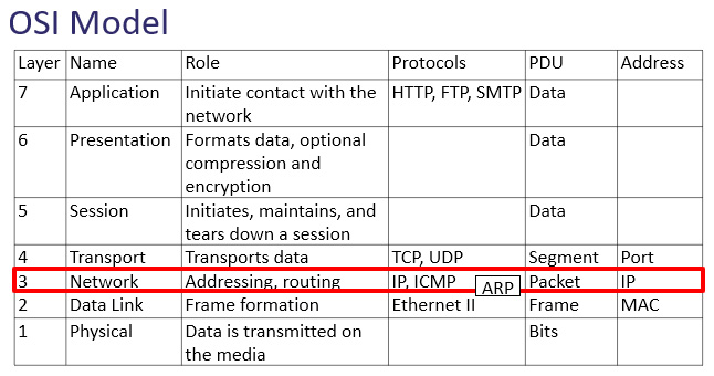
Figure 11.1 – The OSI model—network layer
In addition to IP, the other protocols include the following:
- Address Resolution Protocol (ARP): ARP resolves an IPv4 address (network layer) to a Media Access Control (MAC) (data link layer) address on a local area network so the frame can be delivered to the appropriate host. ARP is shown between layer 3 and layer 2, and as a result, many consider ARP as a layer 3 protocol.
- Internet Control Message Protocol (ICMP): This reports on issues encountered during transit, such as network unreachable or host unreachable.
Next, we'll discuss the role and purpose of IP and how it helps packets find their way when having to pass through networks to reach their final destination.
Understanding the purpose of IP
IP is a network layer protocol that has two key roles: addressing, using a logical IP address, and routing traffic. While the transport layer transports the data, the network layer communicates with other devices to determine the best logical path for the packets.
One of the main protocols in the network layer is IP, which provides a best-effort, connectionless service, as outlined here:
- Best-effort means that there is no guarantee the data will be delivered. It's similar to mailing a letter using general delivery. Although some mail is lost, most of the time it reaches its final destination.
- Connectionless means that IP does not retain any state information; that process is left to the higher-level protocols, such as the Transmission Control Protocol (TCP).
Although IP can't guarantee delivery, it can prioritize traffic, so that time-sensitive data, such as Voice over IP (VoIP) and streaming media, is delivered at a higher precedence than email or web pages.
Because of the unpredictable nature of the internet, prioritizing certain types of traffic will help the data to be delivered faster. The priority is marked in the following ways:
- In IPv4, by using the Differentiated Services (DiffServ) field
- In IPv6, by using the Traffic Class field
To examine the IP headers in detail, we will use the bigFlows.pcap packet capture found at http://tcpreplay.appneta.com/wiki/captures.html#bigflows-pcap. Download the file and open it in Wireshark.
Let's begin with an evaluation of IPv4.
Outlining IPv4
In 1981, Request for Comments (RFC) 791 outlined the specifications for IPv4. The RFC outlined that IPv4 had two principal tasks, addressing and fragmentation, as defined in Section 1.4. Operation, found at https://tools.ietf.org/html/rfc791#section-1.4.
As stated, one of the original roles of IPv4 was fragmentation, which breaks packets apart. At the time, this was necessary because, in the early 1980s, most of the networks had limited bandwidth and were unable to transmit large packets.
Over time, efforts have been made to upgrade and replace the antiquated data pathways, and much of the internet has been replaced by high-speed, fiber optic cables. As a result, in today's networks, fragmentation is rarely used.
Note
Fragmentation is used when the maximum transmission unit (MTU) is less than 1,500 bytes.
As time has passed, we can see that IPv4 is still influential in addressing, along with the role of routing, in order to get data to its final destination.
IPv4 was standardized in 1983 and uses a 32-bit address space. Scientists identified at an early stage the need for a larger address space. IPv6 has a 128-bit address space and provides enhancements to the protocol in general, such as simplified network configuration and more efficient routing. There is a slow migration to IPv6, mainly because the use of private IP addressing on a local area network (LAN) has extended IPv4's lifespan.
As a result, IPv4 is still widely used. So that you have the skills required to face everyday network-related issues when dealing with IPv4, in the next section, we'll examine the IPv4 header and each of the field values. Once you understand the field values, you will be more confident when looking at a packet capture, so you will be able to quickly drill down to the issue.
Dissecting the IPv4 header
The IPv4 header has several fields, as shown in the following diagram:

Figure 11.2 – IPv4 header
Some of the fields are rarely used, such as those that deal with fragmentation. Others provide information that can help with troubleshooting, such as the address fields when resolving network conflicts.
To examine an IPv4 header, open bigFlows.pcap, and go to Frame 1, as shown here:
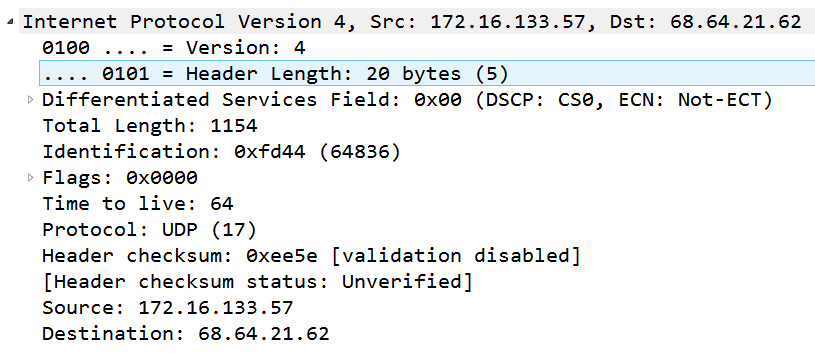
Figure 11.3 – bigFlows Frame 1—IPv4 header
The following section will list each field, how many bits or bytes are used, along with information on what each field represents. We'll start with the version and length fields.
Discovering the version and the length
The first two fields in an IPv4 header are as follows:
- Version (4-bit): This field value indicates the version of IP that is in use. Many devices support both IPv4 and IPv6; therefore, it's important to obtain the version, so the device knows how to treat the traffic. In Frame 1, we see Version: 4, which means this is an IPv4 header.
- Header length (4-bit): The header length is in multiples of 4 bytes and is equal to the base header and any options. Although the length can vary (due to options), the minimum value must be five, which equals a header length of 20 bytes. In Frame 1, the value shows Header Length: 20 bytes (5).
After these two fields, we see a field called DiffServ, which is covered in the next section.
Breaking down the type of service
The internet can be unpredictable, and this can affect time-sensitive data, such as VoIP and streaming media. As a result, IPv4 has the DiffServ field to prioritize time-sensitive traffic, so that it is delivered at a higher precedence than email or web pages.
The DiffServ field is 8 bits and separated into two functions: Quality of Service (QoS) and Explicit Congestion Notification (ECN).
In Frame 1, we can see Differentiated Services Field: 0X00 (DSCP: CSO, ECN: Not-ECT).
As noted, the DiffServ field has two functions. Let's go through what this represents. We'll start with the first 6 bits of the DiffServ field, which is used to represent the QoS requested when traveling through a network.
Ensuring QoS
QoS provides options to prioritize traffic. Most, but not all, devices support QoS. When the priority is requested, the field value will indicate this by using one of several different class selector (CS) values.
For example, CS6 and CS7 are used for network control protocols that include the following:
- Enhanced Interior Gateway Routing Protocol (EIGRP)
- Open Shortest Path First (OSPF)
- Hot Standby Router Protocol (HSRP)
- Internet Key Exchange (IKE)
- Border Gateway Protocol (BGP)
These network protocols are prioritized at a higher level, as any delays will impact network performance.
Other values are as shown in the following table:
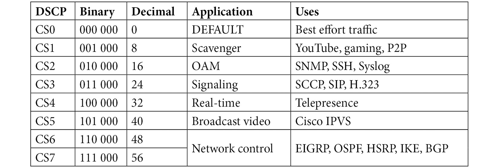
Table 11.1 – Differentiated services field values
The first column shows the Differentiated Services Code Point (DSCP), which lists the CS. As shown in Frame 1, in Figure 11.3, this field value summary shows DSCP: CS0 (or Class Selector 0). CS0 is the default or best-effort setting, in that there is no priority assigned to this packet. Traffic with this setting is delivered normally.
To see an example of a CS that is higher than the best-effort, go to bigFlows.pcap and enter the ip.dsfield.dscp > 0 display filter. Select Frame 4, where you will see the CS value listed, as shown here:

Figure 11.4 – CS1
Class Selector 1 (8) is used in scavenger applications such as YouTube, gaming apps, and P2P, as this traffic would benefit from having a (slightly) higher priority when traveling over the internet.
Note
CS1 is listed as a scavenger application. This class means the application will grab bandwidth whenever it is available
The last 2 bits of the DiffServ field are used to identify ECN, which helps to manage congestion on the network. Let's see how this works.
Sending an ECN
You may not have been aware of ECN and its significance; however, this can have an impact on how devices communicate congestion on the network. Let's take a look at how these 2 bits can improve data flow.
In the original RFC 791, the last 2 bits of the DiffServ field were Reserved for Future Use, as shown in the following screenshot:
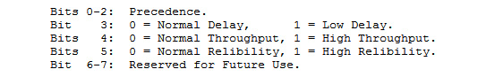
Figure 11.5 – Service bit assignments
In 2001, RFC 3168 found a use for the last 2 bits. RFC 3168 outlined ECN, which provides a congestion notification on the network and is an improvement over the classic method of managing network congestion.
Typically, when TCP experiences congestion, the hosts respond to dropped packets by going into congestion control, which results in the following:
- The client sends duplicate acknowledgments, indicating that there are missing packets.
- The server uses fast retransmission, which resends lost packets.
ECN is an improvement over this behavior by providing a notification that there is congestion on the network. This ultimately prevents the additional traffic that occurs when there are both duplicate acknowledgments and fast retransmissions.
ECN uses both the TCP and IP headers, as outlined here:
- The IP header uses the 2 bits at the end of the DiffServ field to indicate ECN-Capable Transport (ECT) and Congestion Experienced (CE).
- The TCP header uses two flags: Congestion Window Reduced (CWR) and ECN Echo (ECE).
When using ECN, the 2 bits of the DiffServ field identify the code point. In the following table you'll see the bits, what the combination indicates, and what you might see in Wireshark as an indicator when displaying the DiffServ field values:

Table 11.2 – Identifiers in the DiffServ field
As you can see, code points with the values of 10 and 01 are basically the same.
In bigFlows.pcap under Frame 1, if we expand the IPv4 header, we see Explicit Congestion Notification: Not ECN-Capable Transport (0), which means this connection doesn't support ECN, as shown here:

Figure 11.6 – Not ECT-Capable
The devices involved in the connection will communicate with one another and, when available, use ECN, which helps notify endpoints on network congestion issues.
Although IP is a connectionless protocol, it provides methods to improve the priority of traffic, along with ways of notifying devices of congestion issues on the network.
In the next group of field values in the IPv4 header, we'll evaluate the fields that deal with using fragmentation.
Fragmenting the data
In RFC 791, IP was responsible for addressing and fragmentation. We'll discuss addressing in a later section, but for now, let's outline what fragmentation is and why it may be necessary.
On the network, various values are monitored:
- The maximum segment size (MSS) is the data payload.
- The maximum transmission unit (MTU) is the MSS plus the transport layer headers.
When data is routed on the network, it may encounter a segment with an MTU that is smaller than the packet size. If allowed, fragmentation can be used; this divides a datagram into smaller pieces so that they can be sent on the network with a restrictive MTU.
The following three fields are related to fragmentation: identification, flags, and fragment offset, as described here:
- Identification (16-bit): This identification (ID) field is used to identify the datagrams when data is fragmented. In that case, all fragments will have the same ID.
- Flags: In an IP header, there are three flags, as shown in the following screenshot:
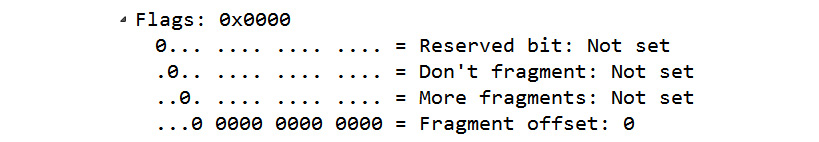
Figure 11.7 – IP flags
- Fragment offset (13-bit): After the three flags in the IP header, this field provides information on how to reassemble the fragments when using fragmentation.
In most cases, the IP header flags will be set at Don't Fragment. That is because in today's networks, fragmentation is not used as most pipelines have generous bandwidth with an acceptable MTU.
Although on today's networks, we rarely see fragmentation, it's a good idea to become familiar with the fields and flags dealing with fragmentation for a couple of scenarios:
- During troubleshooting, you may need to look at the fields when determining why data may not be getting through.
- During a security assessment, the use of the fragmentation fields could be an indication of malicious activity.
Network devices monitor datagram lengths and may impose size restrictions. In that case, if the packet is too large, it may have to be fragmented or rerouted in order to be delivered.
The total length IPv4 field provides a metric when evaluating size restrictions, as it indicates the value of the header length and any data. The field value is 16 bits, which means the entire length cannot exceed 216, or 65,535 bytes.
Internet Control Message Protocol (ICMP) acts as a scout for IP. When ICMP encounters a network with an MTU that is smaller than the size of the packet, and when the Don't Fragment bit is set, the router will drop that packet. ICMP will then notify the source by sending a Type 3 Code 4 ICMP message: Destination Unreachable: Fragmentation Needed and Don't Fragment was Set.
If the packet is dropped on a network segment with restrictive bandwidth that doesn't allow fragmentation, the sending host must retransmit the data using a smaller MSS.
The next few fields are more administrative. They hold values related to the number of hops, the protocol that follows the IPv4 header, and the checksum, which is used for error detection.
Viewing TTL, protocol, and checksum
When looking at the IPv4 header, there are a few fields that are not directly related to routing or addressing packets but provide a role that may influence other types of behavior. Our first example is the Time to Live (TTL) field, which exists because the fathers of the internet realized early on that there must be a way to stop a packet from continually traveling through the network. This can happen if there is a misconfiguration and/or the packet is in a routing loop.
Note
The TTL field is 8 bits, so the maximum value is 28, or 255 hops.
During regular network operations, this most likely won't happen. However, in case there is a routing loop, the TTL field value in an IP header is the number of routers or hops a packet can take before dropping the packet. The TTL works in the following manner:
- Every time the packet reaches a router, the number decrements by 1.
- When the TTL value reaches 0, the packet is dropped and an ICMP Type 11 (TTL expired in transit) is sent to the sender.
To see an example of a TTL value, open bigFlows.pcap, and go to Frame 1, where the TTL field is set at Time to live: 64, which is the default value for this field.
Two other fields that provide information related to managing traffic and informing devices are as follows:
- Protocol (8-bit): The protocol field identifies the higher-layer protocol that follows the IPv4 header. The field identifies the protocol (which is usually a transport layer protocol) that is carried in the datagram. In Frame 1, we see the value as Protocol: UDP (17).
- Header checksum (16-bit): This field is used to house the checksum value. Similar to the checksum in the TCP header, this value is used for error detection. In Frame 1, we see the checksum and notification from Wireshark that the checksum validation is disabled.
Header checksum: 0xee5e [validation disabled]
[Header checksum status: Unverified]
In most cases, it's best to disable validation as the value will be incorrect due to the checksum offloading to the network interface card (NIC).
When dealing with IPv4, there are additional considerations when dealing with addressing, such as special and private IP addresses, as we'll discuss in the following section.
Learning about IPv4 addressing
In this section, we'll examine the last two fields in an IPv4 header. In addition, we'll review the different classes in IPv4, along with an overview of special and private IP addresses.
One of the more significant elements in the IP header is addressing. In the last two fields, we see the source and destination address (32 bits). Each field houses the source or destination IPv4 address, which is represented in an easy-to-understand dotted decimal format. In Frame 1 we see the following values:
Source Address: 172.16.133.57
Destination Address: 68.64.21.62
IPv4 segments the entire address block into classes. Within each class, there are special and private IP addresses. Let's take a look at those concepts.
Comparing IPv4 classes and addresses
When the RFC for IPv4 was written, developers had a concept to subdivide IP into five classes or formats of addresses. IPv4 addresses are divided into classes A-E, as shown here:
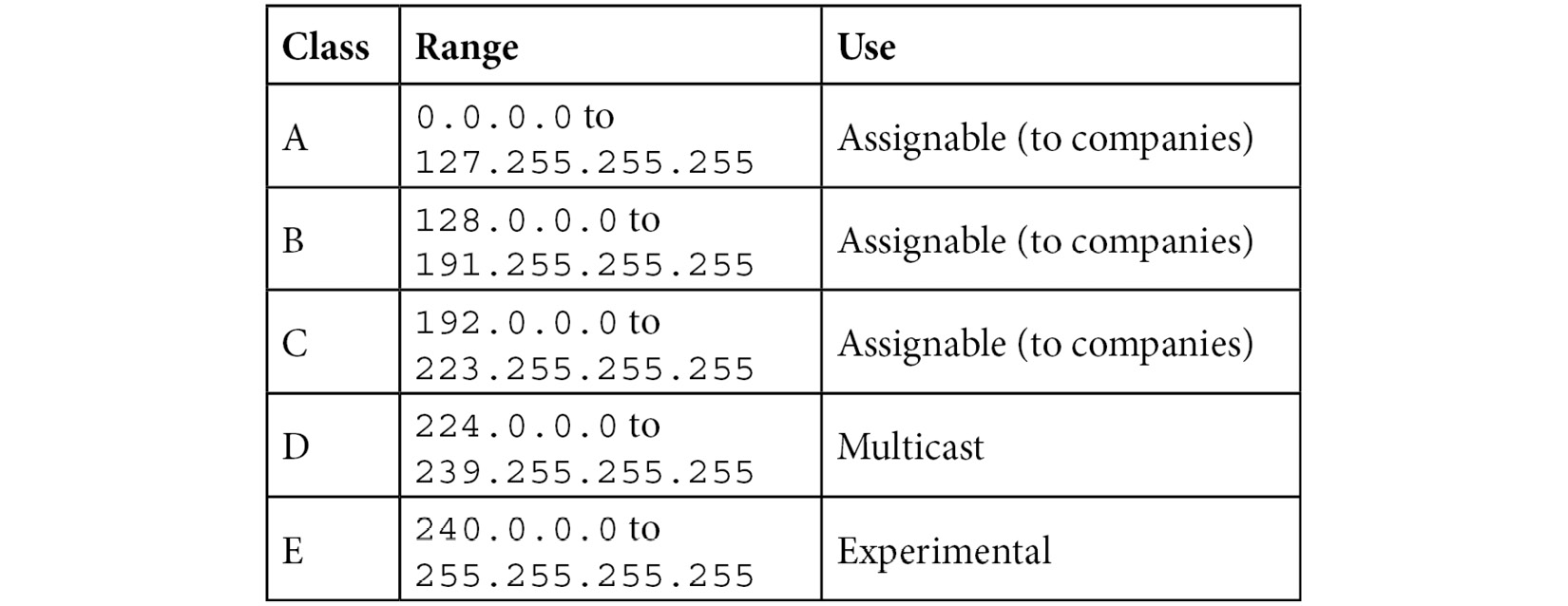
Table 11.3 – Classes of IPv4 addresses
As outlined, classes A, B, and C are assigned mainly to companies. Class D is for multicast only, and class E is experimental, and not used.
In addition to having five classes of addressing, IPv4 has several ranges of special and private IPv4 addresses, as outlined next.
Reviewing special and private IP addressing
One of the limitations of IPv4 is the restrictive address space. To extend the use of IPv4, a group of private IP addresses for classes A, B, and C were drafted, to be used only on an internal network. There is also a generous loopback range and a broadcast IP address.
The following table shows a list of the predominant special and private IPv4 addresses:
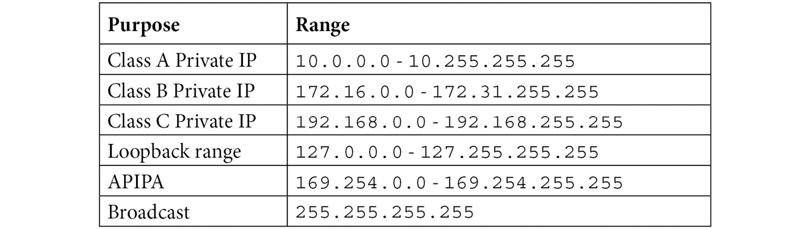
Table 11.4 – Special and private IPv4 addresses
In addition, there is a range for Automatic Private IP Addressing (APIPA), which gives a host an IP address when one isn't available from the Dynamic Host Configuration Protocol (DHCP) server.
While it is rare, options for IPv4 may be used, as discussed in the following section.
Modifying options for IPv4
With IPv4, it may be necessary to use options that provide source routing information, timestamps, and others. Several of the IP options have been deprecated and are no longer used. For a more complete discussion on formally deprecated options, refer to RFC 6814.
When used, the options field must be a multiple of 32 bits, or 4 bytes. Padding may be required so that the header is a multiple of 32 bits.
Now that we have reviewed IPv4, let's take a closer look at IPv6.
Exploring IPv6
Early on, scientists realized that IPv4's 32-bit address space would be exhausted. Although no one had an exact date, plans were made to replace IPv4 with an improved version, IPv6. In 1998, the RFC for IPv6 was published and can be found at https://www.ietf.org/rfc/rfc2460.txt.
IPv6 has a number of enhancements, including the following.
- Streamlined header: The header has fewer fields; however, it is larger, mainly due to the expanded address space.
- Flow label: In IPv6, there is a flow label. The field value is available for identifying streams that require specialized treatment, such as real-time traffic.
- Support for extensions and options: While IPv4 can add options, IPv6 does so with greater ease. IPv6 provides the ability to add options, such as fragmentation, which has parameters to fragment the data, and hop-by-hop, which ensures that all devices in the path read the option.
The IPv6 header has room for larger address spaces. However, as shown in the following diagram, the header is streamlined, in that there are not as many field values:

Figure 11.8 – IPv6 header
To follow along and examine an IPv6 header, open bigFlows.pcap, and go to Frame 347. The IPv6 header is as shown in the following screenshot:
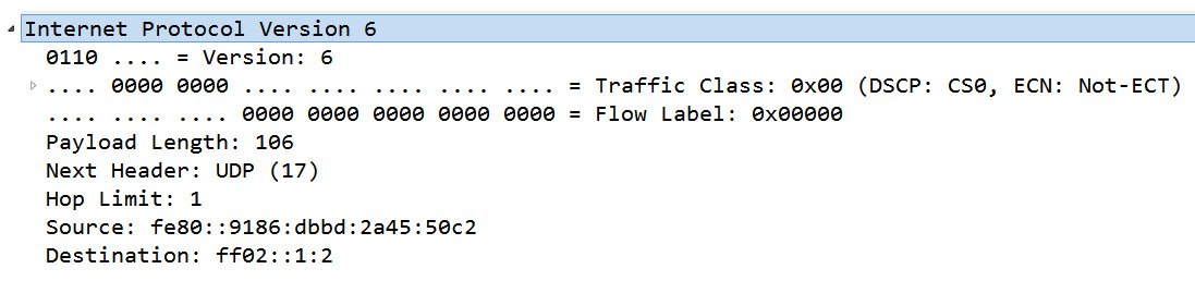
Figure 11.9 – bigFlows frame 347—IPv6 header
Note that IPv6 addresses are significantly larger as they are 128-bit, as opposed to 32-bit for an IPv4 address. The address is shown using hexadecimal notation, as opposed to dotted-decimal notation, which is used in IPv4.
In the next section, we'll review each field in IPv6 and the number of bits or bytes each field contains, along with information on what each field represents.
Navigating the IPv6 header fields
As we'll see, the IPv6 header removes unnecessary field values and adds only what is needed to transport data. Let's step through the field values and learn their significance. We'll start with the version, a field to house the traffic class, and a label dedicated to holding a value for a specific flow.
Identifying the version, traffic class, and flow label
The first three fields in an IPv6 header are as follows:
- Version (4-bit): This field indicates the IP version that is in use. In Frame 347, we see Version 6.
- Traffic class (8-bit): When sending data on the internet, some traffic requires special handling and prioritization. Similar to IPv4, this field houses two values:
- TOS: The first 6 bits of this field are used to communicate what type of service is requested. TOS uses the same DSCP values as IPv4. Frame 347 uses the Differentiated Services Codepoint: Default (0) default value.
- ECN: The last 2 bits of this field are used to indicate congestion on the network in the same way as IPv4. In Frame 347, this value is Explicit Congestion Notification: Not ECN-Capable Transport (0).
- Flow label (20-bit): This field can be used to identify a specific flow of information in order to provide sequencing or request special handling by routers in the path. In Frame 347, we can see Flow Label: 0x00000. In RFC 2460, Appendix A: Semantics and Usage of the Flow Label Field, there is an expanded discussion on the flow label.
As time has passed, we are seeing more use of the flow label. Let's discuss how this is being used, along with examining a populated flow label.
Managing the flow
The label can be used to prioritize traffic, such as real-time data (voice and video), but it can be used for other reasons as well. When used, a randomly assigned number is attached to the flow label, and then all traffic will belong to the same flow or stream.
To see an example of a flow label in use, run a capture on your network, and gather about 1,000 packets. Apply the (!(ipv6.flow == 0x00000)) && (ipv6) filter, which will show only IPv6 packets with a populated flow label.
In addition, you can go to https://wiki.wireshark.org/SampleCaptures#ipv6-and-tunneling-mechanism. Select the sr-header.pcap file and open it in Wireshark.
In this capture, there are 10 packets. Use the ipv6.flow == 0xd684a filter, which will display six packets that are all part of the same flow.
Note
The flow label is a 20-bit field. In Wireshark, you will see the bit values first followed by the hexadecimal value (identified by using 0x before the value). For example, if the field is populated, you will see the following value in Wireshark: .... 1101 0110 1000 0100 1010 = Flow Label: 0xd684a.
The next three fields deal with similar values found in an IPv4 header, but have subtle differences, as shown next.
Evaluating the length, next header, and hop limit
In an IPv6 header, the next three fields provide information on the length of the payload, the protocol that follows the IP header, and how many hops the packet can take before going away. The fields are as follows:
- Payload length (16-bit): The payload length represents the packet's payload, which includes higher-layer headers, data, and any extension headers. Similar to IPv4, the entire length cannot exceed 216, or 65,535 bytes. In some cases, the payload may exceed 65,535 bytes, which can occur when using extension headers. If the value of this is greater than 65,535 bytes, the field value is set to zero (0).
- Next header (8-bit): This field identifies the higher-layer protocol that follows the IP header. This is similar to the protocol field in IPv4 and uses the same values to identify the higher-layer protocol. However, if there is an extension header, this field will indicate what extension header follows the IPv6 header.
- Hop limit (8-bit): In IPv4, the TTL field value in an IP header is the number of routers or hops a packet can take before dropping the packet. In IPv6, this is the same concept. However, the field is more reflective of what it does today. This field uses 8 bits, which can hold a value not greater than 255. If the hop limit reaches 0, the packet is discarded.
In Frame 347, the field value is Hop Limit: 1, which makes sense as this frame is DHCPv6 multicast from a host trying to get an IP address.
As with IPv4, the last two fields in an IPv6 header are the address fields, as discussed next.
Examining IPv6 addresses and address types
IPv6 has specific addressing requirements. In this section, we'll examine the last two fields, source and destination address (128-bit), along with an overview of IPv6 address types. The source and destination addresses are 128-bit fields to accommodate the IPv6 address. Wireshark displays the address in hexadecimal numbers separated by colons, as opposed to dotted-decimal notation, which is used in IPv4.
With IPv6, there are various address types, as opposed to classes. Let's now take a look at the different types you may encounter.
Comparing IPv6 address types
IPv6 does not use a broadcast as in IPv4. However, there are several types of addresses, as listed here:
- Global unicast is like a public IPv4 address. The address is globally recognized and can be routed on the internet.
- Link local is used to communicate with hosts on the same sub-network. This address always starts with FE80.
- Unicast is a single host on a network.
- Multicast packets are delivered to all nodes on a network using a single multicast address.
- Anycast is used to send data to multiple locations with the same IP address. The packets are delivered to the closest (or nearest) destination.
In Frame 347, we see the source and destination addresses:
Source: fe80::9186:dbbd:2a45:50c2
Destination: ff02::1:2
When possible, Wireshark will use appropriate shortcut methods, as shown in the destination address. An IPv6 shortcut removes leading zeros and collapses two or more blocks that contain consecutive zeros.
For many protocols (but not all), Wireshark provides a means to modify the way in which Wireshark presents the data. The following gives us some insight into how to adjust preferences for both IPv4 and IPv6.
Editing protocol preferences
In Wireshark, you can modify most protocols by doing either of the following:
- Right-clicking while on the IP header and selecting Protocol Preferences, where you will see a list of preferences
- Going to Edit | Preferences | Protocols, and then selecting the appropriate protocol
Let's start with the protocol preferences for IPv4, as this is currently the most commonly used protocol on a LAN today.
Reviewing IPv4 preferences
To modify IPv4 preferences, you can use one of the methods listed previously, or you can right-click while on the header and select Protocol Preferences, and then select the Open Internet Protocol Version 4 preferences... shortcut, as shown here:
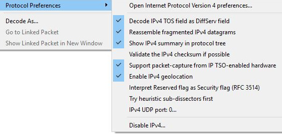
Figure 11.10 – IPv4 preference shortcut
Once you select the shortcut, a list of preferences will be listed, as shown in the following screenshot:
Figure 11.11 – IPv4 preferences
Once there, you can modify the selections as follows:
- Decode IPv4 TOS field as DiffServ field: RFC 791 used TOS to classify traffic. Over time, this field was modified to identify traffic using DiffServ, which allows for a wider range of classification. In most cases, this should be enabled.
- Reassemble fragmented IPv4 datagrams: When necessary, IPv4 packets may be fragmented. When enabled, this will reassemble fragmented IP datagrams.
- Show IPv4 summary in protocol tree: When enabled, this summarizes the header contents. For a large capture, enabling this may impact performance.
- Validate the IPv4 checksum if possible: In most cases, this is not enabled.
- Support packet-capture from IP TSO-enabled hardware: TCP Segmentation Offload (TSO) is a performance-boosting technique used in a virtualized environment. When used, the packet length may be inaccurate. Enabling this option will attempt to correct any errors.
- Enable IPv4 geolocation: Wireshark uses the IP addresses to identify packet origin using the [GeoIP] databases. Select if you want to use this option.
- Interpret Reserved flag as Security flag (RFC 3514): On April 1, 2003 (April Fool's Day), Steven M. Bellovin wrote an RFC that the reserved bit in the IP header should be used by malicious actors to flag the packet if it contains malware, so that IDS and firewalls will know it contains malware. If used, the bit is called the evil bit.
- Try heuristic sub-dissectors first: This option helps Wireshark attempt to identify what type of application is used by using the port number to properly dissect the packet.
- IPv4 UDP port: 0...: Use this option if you want to change the protocol behavior to a specific port when used on the LAN.
- Disable IPv4: Use this option (as shown in Figure 11.10) if you want to disable IPv4 and focus only on the frame headers. Keep in mind if this option is selected, IPv4 and any higher-level protocols (Layers 3-7) will not be dissected.
As you can see, there are many ways to customize the preferences for IPv4. Next, let's take a look at the options for IPv6.
Adjusting preferences for IPv6
You can modify the preferences in IPv6 by going to Edit | Preferences and then selecting the Open Internet Protocol Version 6 preferences... shortcut. This will open a dialog box as shown here:
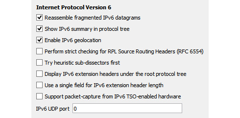
Figure 11.12 – IPv6 preferences
Once there, you can modify any of the options as described here:
- Reassemble fragmented IPv6 datagrams: When enabled, this will reassemble fragmented IPv6 datagrams.
- Show IPv6 summary in protocol tree: When enabled, this summarizes the header contents.
- Enable IPv6 geolocation: Wireshark uses the IP addresses to identify packet origin using the [GeoIP] databases. Select if you want to use this option.
- Perform strict checking for RPL Source Routing Headers (RFC 6554): If enabled, this will aid in troubleshooting streams using Routing Protocol for Low-Power and Lossy Networks (RPL).
- Try heuristic sub-dissectors first: Wireshark will attempt to identify what type of application is used by using the port number to properly dissect the packet.
- Display IPv6 extension headers under the root protocol tree: IPv6 has several extension headers, such as the routing header and the fragment header. Enabling this option will display the headers under the root protocol tree.
- Use a single field for IPv6 extension header length: Enabling this will display a single field for the IPv6 extension header length (if any). If this is not enabled, the field will appear on two lines as follows:
Length: 0 (8 bytes)
[Length: 8 bytes]
- Support packet-capture from IPv6 TSO-enabled hardware: TSO is a performance-boosting technique used in a virtualized environment. When used, the packet length may be inaccurate. Enabling this option will attempt to correct any errors.
- IPv6 UDP port: 0…: Use this option if you want to change the protocol behavior.
The migration from IPv4 to IPv6 has been tepid, as many network administrators continue to use IPv4 on the LAN, mainly because of the flexibility of using private IP addresses. The following section outlines how the two protocols can coexist with one another on the same network, using various tunneling protocols.
Discovering tunneling protocols
Some organizations have decided to make the switch to a dedicated IPv6 networked environment. However, many are running a dual-stack environment, where hosts that are using both IPv4 and IPv6 must be able to communicate with one another.
As evidenced, an IPv4 header is completely different to an IPv6 header. In order to have traffic pass from an IPv4 network through an IPv6 network and vice versa, the traffic must use a tunneling protocol. A discussion of the various ways to transport an IPv6 packet through an IPv4 network is outlined in RFC 7059, found at https://tools.ietf.org/html/rfc7059. The following diagram shows the proper format for encapsulation of an IPv6 packet within an IPv4 packet:
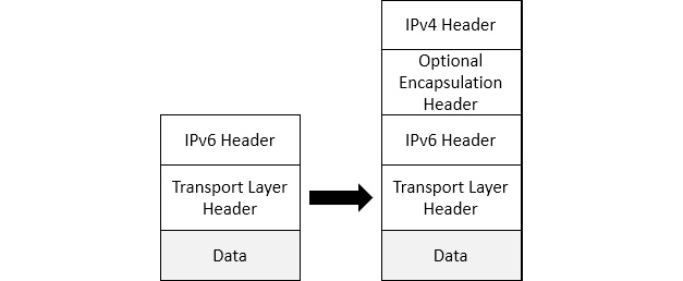
Figure 11.13 – Encapsulation of an IPv6 packet within an IPv4 packet
Some of the tunneling protocols that enable an IPv6 packet to travel over an IPv4 network include the following:
- Intra-Site Automatic Tunnel Addressing Protocol (ISATAP): Transmits data to and from hosts that use IPv6 through an IPv4 network
- Generic Routing Encapsulation (GRE): Creates a point-to-point IPv6 connection within an IPV4 network
- Teredo: Generated in a Windows OS to allow IPv4 hosts to connect to an IPv6 network when network address translation (NAT) is in place.
One of the tunneling protocols, Teredo, wraps (or encapsulates) an IPv6 packet with an IPv4 header so that the packets can travel over an IPv4 environment using NAT. To see an example of Teredo tunneling, go to https://www.cloudshark.org/captures/c0b7d1a1d1ec?filter=frame%20and%20eth%20and%20ip%20and%20udp%20and%20teredo, and open in Wireshark. Go to Frame 29, where we see the IPv6 packet encapsulated in an IPv4 header using UDP as the transport protocol, as shown here:
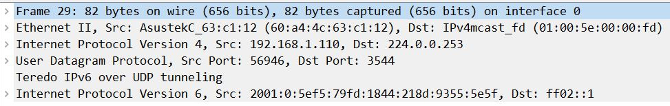
Figure 11.14 – IPv6 packet encapsulated in an IPv4 header
Although there are several tunneling protocols, they all do essentially the same thing: encapsulate one header by using another header, so that data can travel through the network. Because of this, there is additional overhead in creating the tunnel, as well as adding the additional headers.
Because of our complex network environment, you will most likely run into tunneling protocols at some point while troubleshooting your network.
Summary
In this chapter, we started by covering a brief history of IP. We learned how both versions of IP can do the job of routing and addressing; however, there are several differences between the IPv4 and IPv6 headers. We examined and explained each of the field values of both IPv4 and IPv6. Additionally, to give you a better understanding of the two protocols, we compared some of the similarities along with the differences between IPv4 and IPv6.
To help strengthen your knowledge of addressing, we briefly covered the classes of IPv4 addresses, along with reviewing the different types of IPv6 addresses. We then looked at how you can personalize the settings for IPv4 and IPv6 by modifying the protocol preferences. Finally, because of the need for both IP versions to coexist on today's networks, we compared the different types of tunneling protocols in use today.
In the next chapter, we will learn about ICMP, the companion protocol to IP, which works in the network layer of the OSI model. We will evaluate both ICMP, which is used for IPv4, and ICMPv6, which is used with IPv6. We'll then take a deep dive into how ICMP works in both versions, and you will have a better understanding of the two types of messages: error reporting and queries. At the end of the chapter, you'll see how ICMP is the scout for IP and how its use is essential in delivering data.
Questions
Now it's time to check your knowledge. Select the best response, and then check your answers, which can be found in the Assessments appendix:
- Class Selector 6 in the DiffServ field is used with _____.
- Signaling
- Broadcast video
- Network control
- Realtime
- The 172.18.23.119 IP address is a:
- Class C IPv4 address
- Class B private IPv4 address
- Class E IPv4 address
- Class D private IPv6 address
- An IPv6 address has _____ bits.
- 32
- 48
- 64
- 128
- In IPv4, we use a Time to Live value that indicates the number of hops it can take when traveling through the network. In IPv6, this field value is called the _____.
- Router pass
- Class stop
- TTL
- Hop count
- An IPv4 header has _____ flag(s).
- 1
- 2
- 3
- 4
- The following figure shows an IPv6 header. What is the value of the flow label?
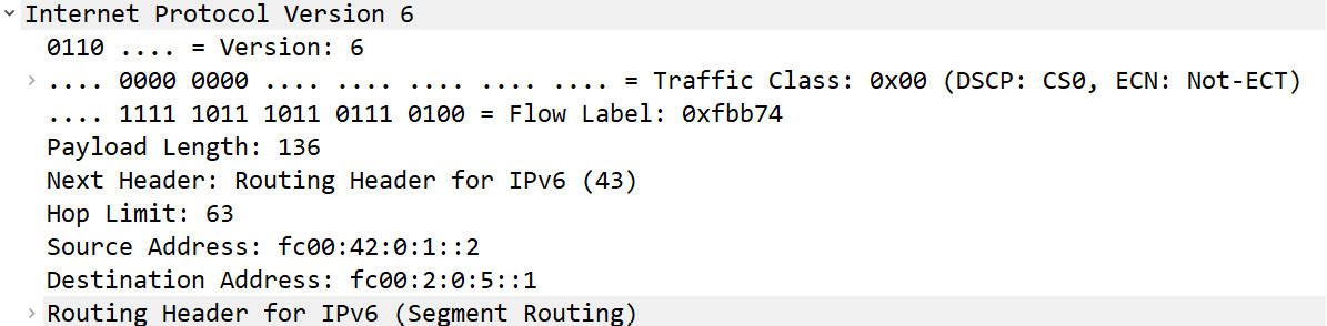
Figure 11.15 – An IPv6 header
- 0X00
- fc00
- 0xfbb74
- 136
- In either an IPv4 or IPv6 header, the payload length cannot exceed _____ bytes.
- 65,535
- 1,111
- 256
- 128
Further reading
Please refer to the following links for more information:
- In 2021, IANA updated the list for the next header field in an IP header. The list can be found at https://www.iana.org/assignments/protocol-numbers/protocol-numbers.xhtml.
- Learn more about RFC 3168 by visiting https://tools.ietf.org/html/rfc3168.
- The TTL value varies as it is OS-dependent. To see the TTL values of various OSs, go to https://subinsb.com/default-device-ttl-values/.
- To view a list of IPv4 options, visit https://www.iana.org/assignments/ip-parameters/ip-parameters.xhtml#ip-parameters-1, which was updated on May 3, 2018.
- A detailed explanation of the IPv6 header can be found at https://www.microsoftpressstore.com/articles/article.aspx?p=2225063&seqNum=3.
- IPv4 has several ranges of special and private IPv4 addresses. To see a complete list, visit https://en.wikipedia.org/wiki/Reserved_IP_addresses.