
Chapter 14: Derived Tables, CTEs, and Views
Derived tables, CTEs, and views are important players in the SQL context. They're useful to organize and optimize the reuse of long and complex queries – typically, base queries and/or expensive queries (in performance terms), and to improve readability by breaking down the code into separate steps. Mainly, they link a certain query to a name, possibly stored in the schema. In other words, they hold the query text, which can be referenced and executed via the associated name when needed. If results materialize, then the database engine can reuse these cached results, otherwise, they have to be recomputed at each call.
Derived tables, CTEs, and views have specific particularities (including database vendor-specific options), and choosing between them is a decision that strongly depends on the use case, the involved data and queries, the database vendor and optimizer, and so on. As usual, we handle this topic from the jOOQ perspective, so our agenda includes the following:
- Derived tables
- CTEs
- Views
Let's get started!
Technical requirements
The code for this chapter can be found on GitHub at https://github.com/PacktPublishing/jOOQ-Masterclass/tree/master/Chapter14.
Derived tables
Have you ever used a nested SELECT (a SELECT in a table expression)? Of course, you have! Then, you've used a so-called derived table having the scope of the statement that creates it. Roughly, a derived table should be treated in the same way as a base table. In other words, it is advisable to give it and its columns meaningful names via the AS operator. This way, you can reference the derived table without ambiguity, and you'll respect the fact that most databases don't support unnamed (unaliased) derived tables.
jOOQ allows us to transform any SELECT in a derived table via asTable(), or its synonym table(). Let's have a simple example starting from this SELECT:
select(inline(1).as("one"));This is not a derived table, but it can become one as follows (these two are synonyms):
Table<?> t = select(inline(1).as("one")).asTable();Table<?> t = table(select(inline(1).as("one")));In jOOQ, we can further refer to this derived table via the local variable t. It is convenient to declare t as Table<?> or to simply use var. But, of course, you can explicitly specify the data types as well. Here, Table<Record1<Integer>>.
Important Note
The org.jooq.Table type can reference a derived table.
Now, the resulting t is an unnamed derived table since there is no explicit alias associated with it. Let's see what happens when we select something from t:
ctx.selectFrom(t).fetch();
jOOQ generates the following SQL (we've arbitrarily chosen the PostgreSQL dialect):
SELECT "alias_30260683"."one"
FROM (SELECT 1 AS "one") AS "alias_30260683"
jOOQ detected the missing alias for the derived table, therefore it generated one (alias_30260683) on our behalf.
Important Note
We earlier iterated that most database vendors require an explicit alias for every derived table. But, as you just saw, jOOQ allows us to omit such aliases, and when we do, jOOQ will generate one on our behalf to guarantee that the generated SQL is syntactically correct. The generated alias is a random number suffixed by alias_. This alias should not be referenced explicitly. jOOQ will use it internally to render a correct/valid SQL.
Of course, if we explicitly specify an alias then jOOQ will use it:
Table<?> t = select(inline(1).as("one")).asTable("t");Table<?> t = table(select(inline(1).as("one"))).as("t");The SQL corresponding to PostgreSQL is as follows:
SELECT "t"."one" FROM (SELECT 1 AS "one") AS "t"
Here is another example using the values() constructor:
Table<?> t = values(row(1, "John"), row(2, "Mary"),
row(3, "Kelly"))
.as("t", "id", "name"); // or, .asTable("t", "id", "name");Typically, we explicitly specify an alias when we also reference it explicitly, but there is nothing wrong in doing it every time. For instance, jOOQ doesn't require an explicit alias for the following inlined derived table, but there is nothing wrong with adding it:
ctx.select()
.from(EMPLOYEE)
.crossApply(select(count().as("sales_count")).from(SALE).where(SALE.EMPLOYEE_NUMBER
.eq(EMPLOYEE.EMPLOYEE_NUMBER)).asTable("t")).fetch();
jOOQ relies on the t alias instead of generating one.
Extracting/declaring a derived table in a local variable
jOOQ allows us to extract/declare a derived table outside the statement that used it, and, in such a case, its presence and role are better outlined than in the case of nesting it in a table expression.
Extracting/declaring a derived table in a local variable can be useful if we need to refer to the derived table in multiple statements, we need it as part of a dynamic query, or we just want to decongest a complex query.
For instance, consider the following query:
ctx.select().from(
select(ORDERDETAIL.PRODUCT_ID, ORDERDETAIL.PRICE_EACH)
.from(ORDERDETAIL)
.where(ORDERDETAIL.QUANTITY_ORDERED.gt(50)))
.innerJoin(PRODUCT)
.on(field(name("price_each")).eq(PRODUCT.BUY_PRICE)).fetch();
The highlighted subquery represents an inlined derived table. jOOQ automatically associates to it an alias and uses that alias to reference the columns product_id and price_each in the outer SELECT. Of course, we can provide an explicit alias as well, but this is not required:
ctx.select().from(
select(ORDERDETAIL.PRODUCT_ID, ORDERDETAIL.PRICE_EACH)
.from(ORDERDETAIL)
.where(ORDERDETAIL.QUANTITY_ORDERED.gt(50))
.asTable("t")).innerJoin(PRODUCT)
.on(field(name("t", "price_each")).eq(PRODUCT.BUY_PRICE)).fetch();
This time, jOOQ relies on the t alias instead of generating one. Next, let's add this subquery to another query as follows:
ctx.select(PRODUCT.PRODUCT_LINE,
PRODUCT.PRODUCT_NAME, field(name("price_each"))).from(select(ORDERDETAIL.PRODUCT_ID,
ORDERDETAIL.PRICE_EACH).from(ORDERDETAIL)
.where(ORDERDETAIL.QUANTITY_ORDERED.gt(50)))
.innerJoin(PRODUCT)
.on(field(name("product_id")).eq(PRODUCT.PRODUCT_ID)).fetch();
This query fails at compilation time because the reference to the product_id column in on(field(name("product_id")).eq(PRODUCT.PRODUCT_ID)) is ambiguous. jOOQ automatically associates a generated alias to the inlined derived table, but it cannot decide whether the product_id column comes from the derived table or from the PRODUCT table. Resolving this issue can be done explicitly by adding and using an alias for the derived table:
ctx.select(PRODUCT.PRODUCT_LINE, PRODUCT.PRODUCT_NAME,
field(name("t", "price_each"))).from(select(ORDERDETAIL.PRODUCT_ID,
ORDERDETAIL.PRICE_EACH).from(ORDERDETAIL)
.where(ORDERDETAIL.QUANTITY_ORDERED.gt(50))
.asTable("t")).innerJoin(PRODUCT)
.on(field(name("t", "product_id")).eq(PRODUCT.PRODUCT_ID))
.fetch();
Now, jOOQ relies on the t alias, and the ambiguity issues have been resolved. Alternatively, we can explicitly associate a unique alias only to the ORDERDETAIL.PRODUCT_ID field as select(ORDERDETAIL.PRODUCT_ID.as("pid")…, and reference it via this alias as field(name("pid"))….
At this point, we have two queries with the same inline derived table. We can avoid code repetition by extracting this derived table in a Java local variable before using it in these two statements. In other words, we declare the derived table in a Java local variable, and we refer to it in the statements via this local variable:
Table<?> t = select(
ORDERDETAIL.PRODUCT_ID, ORDERDETAIL.PRICE_EACH)
.from(ORDERDETAIL)
.where(ORDERDETAIL.QUANTITY_ORDERED.gt(50)).asTable("t");So, t is our derived table. Running this snippet of code doesn't have an effect on and doesn't produce any SQL. jOOQ evaluates t only when we reference it in queries, but in order to be evaluated, t must be declared before the queries that use it. This is just Java; we can use a variable only if it was declared upfront. When a query uses t (for instance, via t.field()), jOOQ evaluates t and renders the proper SQL.
For instance, we can use t to rewrite our queries as follows:
ctx.select()
.from(t)
.innerJoin(PRODUCT)
.on(t.field(name("price_each"), BigDecimal.class).eq(PRODUCT.BUY_PRICE))
.fetch();
ctx.select(PRODUCT.PRODUCT_LINE,
PRODUCT.PRODUCT_NAME, t.field(name("price_each"))).from(t)
.innerJoin(PRODUCT)
.on(t.field(name("product_id"), Long.class).eq(PRODUCT.PRODUCT_ID))
.fetch();
But, why this time do we need explicit types in on(t.field(name("price_each"), BigDecimal.class) and .on(t.field(name("product_id"), Long.class)? The answer is that the fields cannot be dereferenced from t in a type-safe way. Therefore it is our job to specify the proper data types. This is a pure Java issue, and has nothing to do with SQL!
But, there is a trick that can help us to keep type safety and reduce verbosity, and that trick consists of using the <T> Field<T> field(Field<T> field) method. The best explanation of this method is given by the jOOQ documentation itself. The following figure is a screenshot from the jOOQ official documentation:
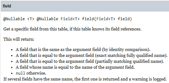
Figure 14.1 – The <T> Field<T> field(Field<T> field) method documentation
The expression t.field(name("price_each"), …) indirectly refers to the field ORDERDETAIL.PRICE_EACH, and t.field(name("product_id"), …) indirectly refers to the field ORDERDETAIL.PRODUCT_ID. Therefore, based on the previous figure, we can re-write our queries in a type-safe manner as follows:
ctx.select(PRODUCT.PRODUCT_LINE, PRODUCT.PRODUCT_NAME,
t.field(ORDERDETAIL.PRICE_EACH))
.from(t)
.innerJoin(PRODUCT)
.on(t.field(ORDERDETAIL.PRODUCT_ID)
.eq(PRODUCT.PRODUCT_ID))
.fetch();
ctx.select()
.from(t)
.innerJoin(PRODUCT)
.on(t.field(ORDERDETAIL.PRICE_EACH)
.eq(PRODUCT.BUY_PRICE))
.fetch();
Cool! Now, we can reuse t in a "type-safe" manner! However, keep in mind that <T> Field<T> field(Field<T> field) just looks type safe. It's actually as good as an unsafe cast in Java, because the lookup only considers the identifier, not the type. Nor does it coerce the expression. This is why we have the quotes around type-safe.
Here is another example that uses two extracted Field in the extracted derived table and the query itself:
// fields
Field<BigDecimal> avg = avg(ORDERDETAIL.PRICE_EACH).as("avg");Field<Long> ord = ORDERDETAIL.ORDER_ID.as("ord");// derived table
Table<?> t = select(avg, ord).from(ORDERDETAIL)
.groupBy(ORDERDETAIL.ORDER_ID).asTable("t");// query
ctx.select(ORDERDETAIL.ORDER_ID, ORDERDETAIL
.ORDERDETAIL_ID,ORDERDETAIL.PRODUCT_ID,
ORDERDETAIL.PRICE_EACH)
.from(ORDERDETAIL, t)
.where(ORDERDETAIL.ORDER_ID.eq(ord)
.and(ORDERDETAIL.PRICE_EACH.lt(avg)))
.orderBy(ORDERDETAIL.ORDER_ID)
.fetch();
Here, ord and avg are rendered unqualified (without being prefixed with the derived table alias). But, thanks to <T> Field<T> field(Field<T> field), we can obtain the qualified version:
...where(ORDERDETAIL.ORDER_ID.eq(t.field(ord))
.and(ORDERDETAIL.PRICE_EACH.lt(t.field(avg))))
...
Next, let's see an example that uses fields() and asterisk() to refer to all columns of a derived table extracted in a local variable:
Table<?> t = ctx.select(SALE.EMPLOYEE_NUMBER,
count(SALE.SALE_).as("sales_count")) .from(SALE).groupBy(SALE.EMPLOYEE_NUMBER).asTable("t");ctx.select(t.fields()).from(t)
.orderBy(t.field(name("sales_count"))).fetch();ctx.select(t.asterisk(),
EMPLOYEE.FIRST_NAME, EMPLOYEE.LAST_NAME)
.from(EMPLOYEE, t)
.where(EMPLOYEE.EMPLOYEE_NUMBER.eq(
t.field(name("employee_number"), Long.class))) .orderBy(t.field(name("sales_count"))).fetch();Notice that extracting a subquery is not mandatory for it to be transformed in a Table. There are cases when extracting it as a simple SELECT is all you need. For instance, when the subquery isn't a derived table, we can do this:
ctx.selectFrom(PRODUCT)
.where(row(PRODUCT.PRODUCT_ID, PRODUCT.BUY_PRICE).in(
select(ORDERDETAIL.PRODUCT_ID, ORDERDETAIL.PRICE_EACH)
.from(ORDERDETAIL)
.where(ORDERDETAIL.QUANTITY_ORDERED.gt(50))))
.fetch();
This subquery (which is not a derived table) can be extracted locally and used like this:
// SelectConditionStep<Record2<Long, BigDecimal>>
var s = select(
ORDERDETAIL.PRODUCT_ID, ORDERDETAIL.PRICE_EACH)
.from(ORDERDETAIL)
.where(ORDERDETAIL.QUANTITY_ORDERED.gt(50));
ctx.selectFrom(PRODUCT)
.where(row(PRODUCT.PRODUCT_ID, PRODUCT.BUY_PRICE).in(s))
.fetch();
There is no need for an alias (jOOQ knows that this is not a derived table and no alias is needed therefore it will not generate one) and no need to transform it into a Table. Actually, jOOQ is so flexible that it allows us to do even this:
var t = select(ORDERDETAIL.PRODUCT_ID, ORDERDETAIL.PRICE_EACH)
.from(ORDERDETAIL)
.where(ORDERDETAIL.QUANTITY_ORDERED.gt(50));
ctx.select(PRODUCT.PRODUCT_LINE, PRODUCT.PRODUCT_NAME,
t.field(ORDERDETAIL.PRICE_EACH))
.from(t)
.innerJoin(PRODUCT)
.on(t.field(ORDERDETAIL.PRODUCT_ID)
.eq(PRODUCT.PRODUCT_ID))
.fetch();
ctx.select()
.from(t)
.innerJoin(PRODUCT)
.on(t.field(ORDERDETAIL.PRICE_EACH)
.eq(PRODUCT.BUY_PRICE))
.fetch();
Don't worry, jOOQ will not ask you to transform t into a Table. jOOQ infers that this is a derived table and associates and references a generated alias as expected in the rendered SQL. So, as long as you don't want to associate an explicit alias to the derived table and jOOQ doesn't specifically require a Table instance in your query, there is no need to transform the extracted SELECT into a Table instance. When you need a Table instance but not an alias for it, just use the asTable() method without arguments:
Table<?> t = select(
ORDERDETAIL.PRODUCT_ID, ORDERDETAIL.PRICE_EACH)
.from(ORDERDETAIL)
.where(ORDERDETAIL.QUANTITY_ORDERED.gt(50)).asTable();
You can check out these examples along with others in DerivedTable.
Exploring Common Table Expressions (CTEs) in jOOQ
CTEs are represented by the SQL-99 WITH clause. You already saw several examples of CTE in previous chapters, for instance, in Chapter 13, Exploiting SQL Functions, you saw a CTE for computing z-scores.
Roughly, via CTEs, we factor out the code that otherwise should be repeated as derived tables. Typically, a CTE contains a list of derived tables placed in front of a SELECT statement in a certain order. The order is important because these derived tables are created conforming to this order and a CTE element can reference only prior CTE elements.
Basically, we distinguish between regular (non-recursive) CTEs and recursive CTEs.
Regular CTEs
A regular CTE associates a name to a temporary result set that has the scope of a statement such as SELECT, INSERT, UPDATE, DELETE, or MERGE (CTEs for DML statements are very useful vendor-specific extensions). But, a derived table or another type of subquery can have its own CTE as well, such as SELECT x.a FROM (WITH t (a) AS (SELECT 1) SELECT a FROM t) x.
The basic syntax of a CTE (for the exact syntax of a certain database vendor, you should consult the documentation) is as follows:
WITH CTE_name [(column_name [, ...])]
AS
(CTE_definition) [, ...]
SQL_statement_using_CTE;
In jOOQ, a CTE is represented by the org.jooq.CommonTableExpression class and extends the commonly used org.jooq.Table, therefore a CTE can be used everywhere a Table can be used. The CTE_name represents the name used later in the query to refer to the CTE and, in jOOQ, can be specified as the argument of the method name() or with().
The column_name marks the spot for a list of comma-separated columns that comes after the CTE_name. The number of columns specified here, and the number of columns defined in the CTE_definition must be equal. In jOOQ, when the name() method is used for CTE_name, this list can be specified via the fields() method. Otherwise, it can be specified as part of the with() arguments after the CTE_name.
The AS keyword is rendered in jOOQ via the as(Select<?> select) method. So, the argument of as() is the CTE_definition. Starting with jOOQ 3.15, the CTE as(ResultQuery<?>) method accepts a ResultQuery<?> to allow for using INSERT ... RETURNING and other DML ... RETURNING statements as CTEs in PostgreSQL.
Finally, we have the SQL that uses the CTE and references it via CTE_name.
For instance, the following CTE named cte_sales computes the sum of sales per employee:
CommonTableExpression<Record2<Long, BigDecimal>> t
= name("cte_sales").fields("employee_nr", "sales").as(select(SALE.EMPLOYEE_NUMBER, sum(SALE.SALE_))
.from(SALE).groupBy(SALE.EMPLOYEE_NUMBER));
This is the CTE declaration that can be referenced via the local variable t in any future SQL queries expressed via jOOQ. Running this snippet of code now doesn't execute the SELECT and doesn't produce any effect. Once we use t in a SQL query, jOOQ will evaluate it to render the expected CTE. That CTE will be executed by the database.
Exactly as in the case of declaring derived tables in local variables, in the case of CTE, the fields cannot be dereferenced from t in a type-safe way, therefore it is our job to specify the proper data types in the queries that use the CTE. Again, let me point out that this is a pure Java issue, and has nothing to do with SQL!
Lukas Eder shared this: Regarding the lack of type safety when dereferencing CTE or derived table fields: This is often an opportunity to rewrite the SQL statement again to something that doesn't use a CTE. On Stack Overflow, I've seen many cases of questions where the person tried to put *everything* in several layers of confusing CTE, when the actual factored-out query could have been *much* easier (for example, if they knew window functions, or the correct logical order of operations, and so on). Just because you can use CTEs, doesn't mean you have to use them *everywhere*.
So, here is a usage of our CTE, t, for fetching the employee having the biggest sales:
ctx.with(t)
.select() // or, .select(t.field("employee_nr"), // t.field("sales")).from(t)
.where(t.field("sales", Double.class) .eq(select(max(t.field("sales" ,Double.class))).from(t))).fetch();
By extracting the CTE fields as local variables, we can rewrite our CTE declaration like this:
Field<Long> e = SALE.EMPLOYEE_NUMBER;
Field<BigDecimal> s = sum(SALE.SALE_);
CommonTableExpression<Record2<Long, BigDecimal>> t
= name("cte_sales").fields(e.getName(), s.getName()).as(select(e, s).from(SALE).groupBy(e));
The SQL that uses this CTE is as follows:
ctx.with(t)
.select() // or, .select(t.field(e.getName()),
// t.field(s.getName()))
.from(t)
.where(t.field(s.getName(), s.getType())
.eq(select(max(t.field(s.getName(), s.getType())))
.from(t))).fetch();
And, of course, relying on <T> Field<T> field(Field<T> field), introduced in the previous section, can help us to write a type-safe CTE as follows:
ctx.with(t)
.select() // or, .select(t.field(e), t.field(s))
.from(t)
.where(t.field(s)
.eq(select(max(t.field(s))).from(t))).fetch();
As an alternative to the previous explicit CTE, we can write an inline CTE as follows:
ctx.with("cte_sales", "employee_nr", "sales").as(select(SALE.EMPLOYEE_NUMBER, sum(SALE.SALE_))
.from(SALE)
.groupBy(SALE.EMPLOYEE_NUMBER))
.select() // or, field(name("employee_nr")), // field(name("sales")) .from(name("cte_sales")) .where(field(name("sales")) .eq(select(max(field(name("sales")))) .from(name("cte_sales")))).fetch();By arbitrarily choosing the PostgreSQL dialect, we have the following rendered SQL for all the previous CTEs:
WITH "cte_sales"("employee_nr", "sales") AS(SELECT "public"."sale"."employee_number",
sum("public"."sale"."sale")FROM "public"."sale"
GROUP BY "public"."sale"."employee_number")
SELECT * FROM "cte_sales"
WHERE "sales" = (SELECT max("sales") FROM "cte_sales")You can check these examples in the bundled code named CteSimple. So far, our CTE is used only in SELECT statements. But, CTE can be used in DML statements such as INSERT, UPDATE, DELETE, and MERGE as well.
CTE as SELECT and DML
jOOQ supports using CTE in INSERT, UPDATE, DELETE, and MERGE. For instance, the following snippet of code inserts into a brand-new table a random part from the SALE table:
ctx.createTableIfNotExists("sale_training").as(selectFrom(SALE)).withNoData().execute();
ctx.with("training_sale_ids", "sale_id").as(select(SALE.SALE_ID).from(SALE)
.orderBy(rand()).limit(10))
.insertInto(table(name("sale_training"))).select(select().from(SALE).where(SALE.SALE_ID.notIn(
select(field(name("sale_id"), Long.class)) .from(name("training_sale_ids"))))).execute();
Here is another example that updates the prices of the products (PRODUCT.BUY_PRICE) to the maximum order prices (max(ORDERDETAIL.PRICE_EACH)) via a CTE used in UPDATE:
ctx.with("product_cte", "product_id", "max_buy_price").as(select(ORDERDETAIL.PRODUCT_ID,
max(ORDERDETAIL.PRICE_EACH))
.from(ORDERDETAIL)
.groupBy(ORDERDETAIL.PRODUCT_ID))
.update(PRODUCT)
.set(PRODUCT.BUY_PRICE, coalesce(field(
select(field(name("max_buy_price"), BigDecimal.class)) .from(name("product_cte")).where(PRODUCT.PRODUCT_ID.eq(
field(name("product_id"), Long.class)))), PRODUCT.BUY_PRICE)).execute();
You can practice these examples along with others including using CTE in DELETE and MERGE in CteSelectDml. Next, let's see how we can express a CTE as DML in PostgreSQL.
A CTE as DML
Starting with jOOQ 3.15, the CTE as(ResultQuery<?>) method accepts a ResultQuery<?> to allow for using INSERT ... RETURNING and other DML … RETURNING statements as CTE in PostgreSQL. Here is a simple CTE storing the returned SALE_ID:
ctx.with("cte", "sale_id").as(insertInto(SALE, SALE.FISCAL_YEAR, SALE.SALE_,
SALE.EMPLOYEE_NUMBER, SALE.FISCAL_MONTH,
SALE.REVENUE_GROWTH)
.values(2005, 1250.55, 1504L, 1, 0.0)
.returningResult(SALE.SALE_ID))
.selectFrom(name("cte")).fetch();
Let's write a CTE that updates the SALE.REVENUE_GROWTH of all employees having a null EMPLOYEE.COMMISSION. All the updated SALE.EMPLOYEE_NUMBER are stored in the CTE and used further to insert in EMPLOYEE_STATUS as follows:
ctx.with("cte", "employee_number").as(update(SALE).set(SALE.REVENUE_GROWTH, 0.0)
.where(SALE.EMPLOYEE_NUMBER.in(
select(EMPLOYEE.EMPLOYEE_NUMBER).from(EMPLOYEE)
.where(EMPLOYEE.COMMISSION.isNull())))
.returningResult(SALE.EMPLOYEE_NUMBER))
.insertInto(EMPLOYEE_STATUS, EMPLOYEE_STATUS
.EMPLOYEE_NUMBER,EMPLOYEE_STATUS.STATUS,
EMPLOYEE_STATUS.ACQUIRED_DATE)
.select(select(field(name("employee_number"), Long.class), val("REGULAR"), val(LocalDate.now())).from(name("cte"))).execute();
You can check out more examples in the bundled code named CteDml for PostgreSQL. Next, let's see how we can embed plain SQL in a CTE.
CTEs and plain SQL
Using plain SQL in CTE is straightforward as you can see in the following example:
CommonTableExpression<Record2<Long, String>>cte = name("cte") .fields("pid", "ppl").as(resultQuery(// Put any plain SQL statement here
"""
select "public"."product"."product_id",
"public"."product"."product_line"
from "public"."product"
where "public"."product"."quantity_in_stock" > 0
"""
).coerce(field("pid", BIGINT), field("ppl", VARCHAR)));Result<Record2<Long, String>> result =
ctx.with(cte).selectFrom(cte).fetch();
You can test this example in the bundled code named CtePlainSql. Next, let's tackle some common types of CTEs, and let's continue with a query that uses two or more CTEs.
Chaining CTEs
Sometimes, a query must exploit more than one CTE. For instance, let's consider the tables PRODUCTLINE, PRODUCT, and ORDERDETAIL. Our goal is to fetch for each product line some info (for instance, the description), the total number of products, and the total sales. For this, we can write a CTE that joins PRODUCTLINE with PRODUCT and count the total number of products per product line, and another CTE that joins PRODUCT with ORDERDETAIL and computes the total sales per product line. Then, both CTEs are used in a SELECT to fetch the final result as in the following inlined CTE:
ctx.with("cte_productline_counts").as(select(PRODUCT.PRODUCT_LINE, PRODUCT.CODE,
count(PRODUCT.PRODUCT_ID).as("product_count"), PRODUCTLINE.TEXT_DESCRIPTION.as("description")).from(PRODUCTLINE).join(PRODUCT).onKey()
.groupBy(PRODUCT.PRODUCT_LINE, PRODUCT.CODE,
PRODUCTLINE.TEXT_DESCRIPTION))
.with("cte_productline_sales").as(select(PRODUCT.PRODUCT_LINE,
sum(ORDERDETAIL.QUANTITY_ORDERED
.mul(ORDERDETAIL.PRICE_EACH)).as("sales")).from(PRODUCT).join(ORDERDETAIL).onKey()
.groupBy(PRODUCT.PRODUCT_LINE))
.select(field(name("cte_productline_counts", "product_line")), field(name("code")), field(name("product_count")), field(name("description")), field(name("sales"))) .from(name("cte_productline_counts")) .join(name("cte_productline_sales")) .on(field(name("cte_productline_counts", "product_line"))
.eq(field(name("cte_productline_sales", "product_line"))))
.orderBy(field(name("cte_productline_counts", "product_line")))
.fetch();
In the bundled code (CteSimple), you can see the explicit CTE version as well.
Nested CTEs
CTEs can be nested as well. For instance, here we have a "base" CTE that computes the employees' average salary per office. The next two CTEs fetch from the "base" CTE the minimum and maximum average respectively. Finally, our query cross-joins these CTEs:
ctx.with("avg_per_office") .as(select(EMPLOYEE.OFFICE_CODE.as("office"), avg(EMPLOYEE.SALARY).as("avg_salary_per_office")).from(EMPLOYEE)
.groupBy(EMPLOYEE.OFFICE_CODE))
.with("min_salary_office") .as(select(min(field(name("avg_salary_per_office"))) .as("min_avg_salary_per_office")) .from(name("avg_per_office"))) .with("max_salary_office") .as(select(max(field(name("avg_salary_per_office"))) .as("max_avg_salary_per_office")) .from(name("avg_per_office"))).select()
.from(name("avg_per_office")) .crossJoin(name("min_salary_office")) .crossJoin(name("max_salary_office")).fetch();
The potential output is shown in the next figure:
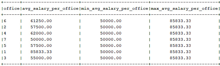
Figure 14.2 – Output of nested CTEs example
In the bundled code (CteSimple), you can see the explicit CTE version as well.
Some databases (for instance, MySQL and PostgreSQL) allow you to nest CTEs via the FROM clause. Here is an example:
ctx.with("t2") .as(select(avg(field("sum_min_sal", Float.class)) .as("avg_sum_min_sal")).from( with("t1") .as(select(min(EMPLOYEE.SALARY).as("min_sal")).from(EMPLOYEE)
.groupBy(EMPLOYEE.OFFICE_CODE)).select(
sum(field("min_sal", Float.class)) .as("sum_min_sal")) .from(name("t1")) .groupBy(field("min_sal")))).select()
.from(name("t2")).fetch();
So, this is a three-step query: first, we compute the minimum salary per office; second, we compute the sum of salaries per minimum salary; and third, we compute the average of these sums.
Materialized CTEs
Do you have an expensive CTE that fetches a relatively small result set and is used two or more times? Then most probably you have a CTE that you may want to materialize. The materialized CTE can then be referenced multiple times by the parent query without recomputing the results.
In jOOQ, materializing a CTE can be done via asMaterialized(). Depending on the database, jOOQ will render the proper SQL. For instance, consider the following materialized CTE:
ctx.with("cte", "customer_number", "order_line_number", "sum_price", "sum_quantity")
.asMaterialized(
select(ORDER.CUSTOMER_NUMBER,
ORDERDETAIL.ORDER_LINE_NUMBER,
sum(ORDERDETAIL.PRICE_EACH),
sum(ORDERDETAIL.QUANTITY_ORDERED))
.from(ORDER)
.join(ORDERDETAIL)
.on(ORDER.ORDER_ID.eq(ORDERDETAIL.ORDER_ID))
.groupBy(ORDERDETAIL.ORDER_LINE_NUMBER,
ORDER.CUSTOMER_NUMBER))
.select(field(name("customer_number")), inline("Order Line Number").as("metric"), field(name("order_line_number"))).from(name("cte")) // 1 .unionAll(select(field(name("customer_number")), inline("Sum Price").as("metric"), field(name("sum_price"))).from(name("cte"))) // 2 .unionAll(select(field(name("customer_number")), inline("Sum Quantity").as("metric"), field(name("sum_quantity"))).from(name("cte"))) // 3 .fetch();
This CTE should be evaluated three times (denoted in code as //1, //2, and //3). Hopefully, thanks to asMaterialized(), the result of the CTE should be materialized and reused instead of being recomputed.
Some databases detect that a CTE is used more than once (the WITH clause is referenced more than once in the outer query) and automatically try to materialize the result set as an optimization fence. For instance, PostgreSQL will materialize the above CTE even if we don't use asMaterialized() and we simply use as() because the WITH query is called three times.
But, PostgreSQL allows us to control the CTE materialization and change the default behavior. If we want to force inlining the CTE instead of it being materialized, then we add the NOT MATERIALIZED hint to the CTE. In jOOQ, this is accomplished via asNotMaterialized():
ctx.with("cte", "customer_number", "order_line_number", "sum_price", "sum_quantity")
.asNotMaterialized(select(ORDER.CUSTOMER_NUMBER,
ORDERDETAIL.ORDER_LINE_NUMBER, ...
On the other hand, in Oracle, we can control materialization via the /*+ materialize */ and /*+ inline */ hints. Using jOOQ's asMaterialized() renders the /*+ materialize */ hint, while asNotMaterialized() renders the /*+ inline */ hint. Using jOOQ's as() doesn't render any hint, so Oracle's optimizer is free to act as the default.
However, Lukas Eder said: Note that the Oracle hints aren't documented, so they might change (though all possible Oracle guru blogs document their de facto functionality, so knowing Oracle, they won't break easily). If not explicitly documented, there's never any *guarantee* for any *materialization trick* to keep working.
Other databases don't support materialization at all or use it only as an internal mechanism of the optimizer (for instance, MySQL). Using jOOQ's as(), asMaterialized(), and asNotMaterialized() renders the same SQL for MySQL, therefore we cannot rely on explicit materialization. In such cases, we can attempt to rewrite our CTE to avoid recalls. For instance, the previous CTE can be optimized to not need materialization in MySQL via LATERAL:
ctx.with("cte").as(
select(ORDER.CUSTOMER_NUMBER,
ORDERDETAIL.ORDER_LINE_NUMBER,
sum(ORDERDETAIL.PRICE_EACH).as("sum_price"),sum(ORDERDETAIL.QUANTITY_ORDERED)
.as("sum_quantity")).from(ORDER)
.join(ORDERDETAIL)
.on(ORDER.ORDER_ID.eq(ORDERDETAIL.ORDER_ID))
.groupBy(ORDERDETAIL.ORDER_LINE_NUMBER,
ORDER.CUSTOMER_NUMBER))
.select(field(name("customer_number")), field(name("t", "metric")), field(name("t", "value"))) .from(table(name("cte")), lateral( select(inline("Order Line Number").as("metric"), field(name("order_line_number")).as("value")) .unionAll(select(inline("Sum Price").as("metric"), field(name("sum_price")).as("value"))) .unionAll(select(inline("Sum Quantity").as("metric"), field(name("sum_quantity")).as("value")))) .as("t")).fetch();Here is the alternative for SQL Server (like MySQL, SQL Server doesn't expose any support for explicit materialization; however, there is a proposal for Microsoft to add a dedicated hint similar to what Oracle has) using CROSS APPLY and the VALUES constructor:
ctx.with("cte").as(select(ORDER.CUSTOMER_NUMBER,
ORDERDETAIL.ORDER_LINE_NUMBER,
sum(ORDERDETAIL.PRICE_EACH).as("sum_price"),sum(ORDERDETAIL.QUANTITY_ORDERED)
.as("sum_quantity")).from(ORDER)
.join(ORDERDETAIL)
.on(ORDER.ORDER_ID.eq(ORDERDETAIL.ORDER_ID))
.groupBy(ORDERDETAIL.ORDER_LINE_NUMBER,
ORDER.CUSTOMER_NUMBER))
.select(field(name("customer_number")), field(name("t", "metric")), field(name("t", "value"))) .from(name("cte")).crossApply( values(row("Order Line Number", field(name("cte", "order_line_number"))), row("Sum Price", field(name("cte", "sum_price"))), row("Sum Quantity", field(name("cte", "sum_quantity")))) .as("t", "metric", "value")).fetch();A good cost-based optimizer should always rewrite all SQL statements to the optimal execution plan, so what may work today, might not work tomorrow – such as this LATERAL/CROSS APPLY trick. If the optimizer is ever smart enough to detect that LATERAL/CROSS APPLY is unnecessary (for example, because of the lack of correlation), then it might be (should be) eliminated.
You can check out all these examples in CteSimple. Moreover, in the CteAggRem application, you can practice a CTE for calculating the top N items and aggregating (summing) the remainder in a separate row. Basically, while ranking items in the database is a common problem to compute top/bottom N items, another common requirement that is related to this one is to obtain all the other rows (that don't fit in top/bottom N) in a separate row. This is helpful to provide a complete context when presenting data.
In the CteWMAvg code, you can check out a statistics problem with the main goal being to highlight recent points. This problem is known as Weighted Moving Average (WMA). This is part of the moving average family (https://en.wikipedia.org/wiki/Moving_average) and, in a nutshell, WMA is a moving average where the previous values (points) range in the sliding window are given different (fractional) weights.
Recursive CTEs
Besides regular CTEs, we have recursive CTEs.
In a nutshell, recursive CTEs reproduce the concept of for-loops in programming. A recursive CTE can handle and explore hierarchical data by referencing themselves. Behind a recursive CTE, there are two main members:
- The anchor member – Its goal is to select the starting rows of the involved recursive steps.
- The recursive member – Its goal is to generate rows for the CTE. The first iteration step acts against the anchor rows, while the second iteration step acts against the rows previously created in recursions steps. This member occurs after a UNION ALL in the CTE definition part. To be more accurate, UNION ALL is required by a few dialects, but others are capable of recurring with UNION as well, with slightly different semantics.
In jOOQ, recursive CTEs can be expressed via the withRecursive() method.
Here's a simple recursive CTE that computes the famous Fibonacci numbers. The anchor member is equal to 1, and the recursive member applies the Fibonacci formula up to the number 20:
ctx.withRecursive("fibonacci", "n", "f", "f1").as(select(inline(1L), inline(0L), inline(1L))
.unionAll(select(field(name("n"), Long.class).plus(1), field(name("f"), Long.class).plus(field(name("f1"))), field(name("f"), Long.class)) .from(name("fibonacci")) .where(field(name("n")).lt(20)))) .select(field(name("n")), field(name("f")).as("f_nbr")) .from(name("fibonacci")).fetch();
Well, that was easy, wasn't it? Next, let's tackle a famous problem that can be solved via recursive CTE, known as the Travelling Salesman Problem. Consider reading more details here: https://en.wikipedia.org/wiki/Travelling_salesman_problem. In a nutshell, we interpret this problem to find the shortest private flight through several cities representing locations of our offices. Basically, in OFFICE_FLIGHTS, we have the routes between our offices as OFFICE_FLIGHTS.DEPART_TOWN, OFFICE_FLIGHTS.ARRIVAL_TOWN, and OFFICE_FLIGHTS.DISTANCE_KM. For instance, our CTE will use Los Angeles as its anchor city, and then recursively traverse every other city in order to reach Tokyo:
String from = "Los Angeles";
String to = "Tokyo";
ctx.withRecursive("flights", "arrival_town", "steps", "total_distance_km", "path")
.as(selectDistinct(OFFICE_FLIGHTS.DEPART_TOWN
.as("arrival_town"), inline(0).as("steps"), inline(0) .as("total_distance_km"), cast(from, SQLDataType.VARCHAR) .as("path")).from(OFFICE_FLIGHTS)
.where(OFFICE_FLIGHTS.DEPART_TOWN.eq(from))
.unionAll(select(field(name("arrivals", "arrival_town"), String.class), field(name("flights", "steps"), Integer.class).plus(1), field(name("flights", "total_distance_km"), Integer.class).plus(
field(name("arrivals", "distance_km"))), concat(field(name("flights", "path")),inline(","), field(name("arrivals", "arrival_town")))) .from(OFFICE_FLIGHTS.as("arrivals"), table(name("flights"))) .where(field(name("flights", "arrival_town")) .eq(field(name("arrivals", "depart_town"))) .and(field(name("flights", "path")) .notLike(concat(inline("%"), field(name("arrivals", "arrival_town")), inline("%"))))))).select()
.from(name("flights")) .where(field(name("arrival_town")).eq(to)) .orderBy(field(name("total_distance_km"))).fetch();
Some possible output is in the next figure:
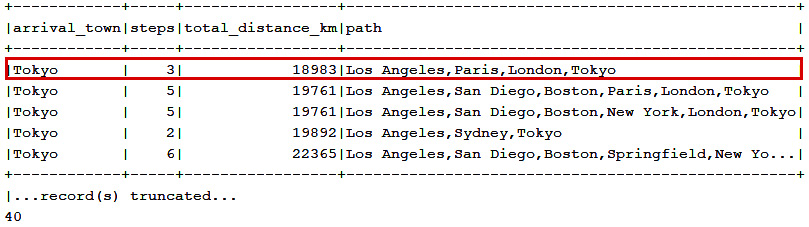
Figure 14.3 – Shortest private flight from Los Angeles to Tokyo, 18,983 km
You can practice these examples in CteRecursive.
CTEs and window functions
In this section, let's look at two examples that combine CTE and window functions, and let's start with an example that computes the gaps in IDs. For instance, each EMPLOYEE has an associated EMPLOYEE_NUMBER and we want to find out how many values are missing from the data values (missing EMPLOYEE_NUMBER), and how many existing values are consecutive. This is a job for the ROW_NUMBER() window and the following CTE:
ctx.with("t", "data_val", "data_seq", "absent_data_grp").as(select(EMPLOYEE.EMPLOYEE_NUMBER,
rowNumber().over()
.orderBy(EMPLOYEE.EMPLOYEE_NUMBER)))
EMPLOYEE.EMPLOYEE_NUMBER.minus(
rowNumber().over()
.orderBy(EMPLOYEE.EMPLOYEE_NUMBER)))
.from(EMPLOYEE))
.select(field(name("absent_data_grp")), count(), min(field(name("data_val"))).as("start_data_val")) .from(name("t")) .groupBy(field(name("absent_data_grp"))) .orderBy(field(name("absent_data_grp"))).fetch();
While you can see this example in the bundled code, let's look at another one that finds the percentile rank of every product line by order values:
ctx.with("t", "product_line", "sum_price_each").as(select(PRODUCT.PRODUCT_LINE,
sum(ORDERDETAIL.PRICE_EACH))
.from(PRODUCT)
.join(ORDERDETAIL)
.on(PRODUCT.PRODUCT_ID.eq(ORDERDETAIL.PRODUCT_ID))
.groupBy(PRODUCT.PRODUCT_LINE))
.select(field(name("product_line")), field(name("sum_price_each")),round(percentRank().over()
.orderBy(field(name("sum_price_each"))).mul(100), 2) .concat("%").as("percentile_rank")) .from(name("t")).fetch();
You can find these examples along with another one that finds the top three highest-valued orders each year in CteWf.
Using CTEs to generate data
CTEs are quite handy for generating data – they act as the source of data for the SQL statement that uses a CTE. For instance, using a CTE and the VALUES constructor can be done as follows:
ctx.with("dt").as(select()
.from(values(row(1, "John"), row(2, "Mary"), row(3, "Kelly"))
.as("t", "id", "name"))).select()
.from(name("dt")).fetch();
Or, using a CTE to unnest an array can be done as follows:
ctx.with("dt").as(select().from(unnest(new String[]
{"John", "Mary", "Kelly"}).as("n"))).select()
.from(name("dt")).fetch();
Or, here is an example of unnesting an array to pick up a random value:
ctx.with("dt").as(select().from(unnest(new String[]
{"John", "Mary", "Kelly"}).as("n"))).select()
.from(name("dt")).orderBy(rand())
.limit(1)
.fetch();
Or, maybe you need a random sample from the database (here, 10 random products):
ctx.with("dt").as(selectFrom(PRODUCT).orderBy(rand()).limit(10))
.select()
.from(name("dt")).fetch();
However, keep in mind that ORDER BY RAND() should be avoided for large tables, as ORDER BY performs with O(N log N).
If you need more sophisticated sources of data, then probably you'll be interested in generating a series. Here is an example of generating the odd numbers between 1 and 10:
ctx.with("dt") .as(select().from(generateSeries(1, 10, 2).as("t", "s"))).select()
.from(name("dt")).fetch();
Here is an example that associates grades between 1 and 100 with the letters A to F and counts them as well – in other words, custom binning of grades:
ctx.with("grades").as(select(round(inline(70).plus(sin(
field(name("serie", "sample"), Integer.class)) .mul(30))).as("grade")) .from(generateSeries(1, 100).as("serie", "sample"))).select(
case_().when(field(name("grade")).lt(60), "F") .when(field(name("grade")).lt(70), "D") .when(field(name("grade")).lt(80), "C") .when(field(name("grade")).lt(90), "B") .else_("A").as("letter_grade"),count()) .from(name("grades")) .groupBy(field(name("letter_grade"))) .orderBy(field(name("letter_grade"))).fetch();
In the bundled code, you can see more binning examples including custom binning of grades via PERCENT_RANK(), equal height binning, equal-width binning, the PostgreSQL width_bucket() function, and binning with a chart.
After all these snippets, let's tackle the following famous problem: Consider p student classes of certain sizes, and q rooms of certain sizes, where q>= p. Write a CTE for assigning as many classes as possible to rooms of proper size. Let's assume that the given data is in the left-hand side figure and the expected result is in the right-hand side figure:

Figure 14.4 – Input and expected output
In order to solve this problem, we can generate the input data as follows:
ctx.with("classes").as(select()
.from(values(row("c1", 80), row("c2", 70), row("c3", 65), row("c4", 55), row("c5", 50), row("c6", 40)) .as("t", "class_nbr", "class_size"))) .with("rooms").as(select()
.from(values(row("r1", 70), row("r2", 40), row("r3", 50), row("r4", 85), row("r5", 30), row("r6", 65), row("r7", 55)) .as("t", "room_nbr", "room_size")))…
The complete query is quite large to be listed here, but you can find it in the CteGenData application next to all the examples from this section.
Dynamic CTEs
Commonly, when we need to dynamically create a CTE, we plan to dynamically shape its name, derived table(s), and the outer query. For instance, the following method allows us to pass these components as arguments and return the result of executing the query:
public Result<Record> cte(String cteName, Select select,
SelectField<?>[] fields, Condition condition,
GroupField[] groupBy, SortField<?>[] orderBy) {var cte = ctx.with(cteName).as(select);
var cteSelect = fields == null
? cte.select() : cte.select(fields)
.from(table(name(cteName)));
if (condition != null) {cteSelect.where(condition);
}
if (groupBy != null) {cteSelect.groupBy(groupBy);
}
if (orderBy != null) {cteSelect.orderBy(orderBy);
}
return cteSelect.fetch();
}
Here is a calling sample for solving the problem presented earlier, in the CTEs and window functions section:
Result<Record> result = cte("t", select(EMPLOYEE.EMPLOYEE_NUMBER.as("data_val"),rowNumber().over().orderBy(EMPLOYEE.EMPLOYEE_NUMBER)
.as("data_seq"), EMPLOYEE.EMPLOYEE_NUMBER.minus(rowNumber().over().orderBy(EMPLOYEE.EMPLOYEE_NUMBER))
.as("absent_data_grp")).from(EMPLOYEE),
new Field[]{field(name("absent_data_grp")), count(), min(field(name("data_val"))).as("start_data_val")}, null, new GroupField[]{field(name("absent_data_grp"))},null);
Whenever you try to implement a CTE, as here, consider this Lukas Eder note: This example uses the DSL in a mutable way, which works but is discouraged. A future jOOQ version might turn to an immutable DSL API and this code will stop working. It's unlikely to happen soon, because of the huge backward incompatibility, but the discouragement is real already today :) In IntelliJ, you should already get a warning in this code, because of the API's @CheckReturnValue annotation usage, at least in jOOQ 3.15.
On the other hand, if you just need to pass a variable number of CTEs to the outer query, then you can do this:
public void CTE(List<CommonTableExpression<?>> CTE) {ctx.with(CTE)
...
}
Or, you can do this:
public void CTE(CommonTableExpression<?> cte1,
CommonTableExpression<?>cte2,
CommonTableExpression<?>cte3, ...) {ctx.with(cte1, cte2, cte3)
...
}
You can practice these examples in CteDynamic.
Expressing a query via a derived table, a temporary table, and a CTE
Sometimes, we prefer to express a query in several ways to compare their execution plans. For instance, we may have a query and express it via derived tables, temporary tables, and CTE to see which approach fits best. Since jOOQ supports these approaches, let's try to express a query starting from the derived tables approach:
ctx.select(EMPLOYEE.FIRST_NAME, EMPLOYEE.LAST_NAME,
sum(SALE.SALE_), field(select(sum(SALE.SALE_)).from(SALE))
.divide(field(select(countDistinct(SALE.EMPLOYEE_NUMBER))
.from(SALE))).as("avg_sales")).from(EMPLOYEE)
.innerJoin(SALE)
.on(EMPLOYEE.EMPLOYEE_NUMBER.eq(SALE.EMPLOYEE_NUMBER))
.groupBy(EMPLOYEE.FIRST_NAME, EMPLOYEE.LAST_NAME)
.having(sum(SALE.SALE_).gt(field(select(sum(SALE.SALE_))
.from(SALE))
.divide(field(select(countDistinct(SALE.EMPLOYEE_NUMBER))
.from(SALE))))).fetch();
So, this query returns all employees with above-average sales. For each employee, we compare their average sales to the total average sales for all employees. Essentially, this query works on the EMPLOYEE and SALE tables, and we must know the total sales for all employees, the number of employees, and the sum of sales for each employee.
If we extract what we must know in three temporary tables, then we obtain this:
ctx.createTemporaryTable("t1").as( select(sum(SALE.SALE_).as("sum_all_sales")).from(SALE)).execute();
ctx.createTemporaryTable("t2").as(select(countDistinct(SALE.EMPLOYEE_NUMBER)
.as("nbr_employee")).from(SALE)).execute();ctx.createTemporaryTable("t3").as(select(EMPLOYEE.FIRST_NAME, EMPLOYEE.LAST_NAME,
sum(SALE.SALE_).as("employee_sale")).from(EMPLOYEE)
.innerJoin(SALE)
.on(EMPLOYEE.EMPLOYEE_NUMBER.eq(SALE.EMPLOYEE_NUMBER))
.groupBy(EMPLOYEE.FIRST_NAME, EMPLOYEE.LAST_NAME))
.execute();
Having these three temporary tables, we can rewrite our query as follows:
ctx.select(field(name("first_name")),field(name("last_name")), field(name("employee_sale")), field(name("sum_all_sales")) .divide(field(name("nbr_employee"), Integer.class)) .as("avg_sales")) .from(table(name("t1")),table(name("t2")), table(name("t3"))) .where(field(name("employee_sale")).gt( field(name("sum_all_sales")).divide( field(name("nbr_employee"), Integer.class)))).fetch();
Finally, the same query can be expressed via CTE (by replacing as() with asMaterialized(), you can practice the materialization of this CTE):
ctx.with("cte1", "sum_all_sales").as(select(sum(SALE.SALE_)).from(SALE))
.with("cte2", "nbr_employee").as(select(countDistinct(SALE.EMPLOYEE_NUMBER)).from(SALE))
.with("cte3", "first_name", "last_name", "employee_sale").as(select(EMPLOYEE.FIRST_NAME, EMPLOYEE.LAST_NAME,
sum(SALE.SALE_).as("employee_sale")).from(EMPLOYEE)
.innerJoin(SALE)
.on(EMPLOYEE.EMPLOYEE_NUMBER.eq(SALE.EMPLOYEE_NUMBER))
.groupBy(EMPLOYEE.FIRST_NAME, EMPLOYEE.LAST_NAME))
.select(field(name("first_name")), field(name("last_name")), field(name("employee_sale")), field(name("sum_all_sales")) .divide(field(name("nbr_employee"), Integer.class)) .as("avg_sales")) .from(table(name("cte1")), table(name("cte2")), table(name("cte3"))) .where(field(name("employee_sale")).gt( field(name("sum_all_sales")).divide( field(name("nbr_employee"), Integer.class)))).fetch();
Now you just have to run these queries against your database and compare their performances and execution plans. The bundled code contains one more example and is available as ToCte.
Handling views in jOOQ
The last section of this chapter is reserved for database views.
A view acts as an actual physical table that can be invoked by name. They fit well for reporting tasks or integration with third-party tools that need a guided query API. By default, the database vendor decides to materialize the results of the view or to rely on other mechanisms to get the same effect. Most vendors (hopefully) don't default to materializing views! Views should behave just like CTE or derived tables and should be transparent to the optimizer. In most cases (in Oracle), we would expect a view to be inlined, even when selected several times, because each time, a different predicate might be pushed down into the view. Actual materialized views are supported only by a few vendors, while the optimizer can decide to materialize the view contents when a view is queried several times. The view's definition is stored in the schema tables so it can be invoked by name wherever a regular/base table could be used. If the view is updatable, then some additional rules come to sustain it.
A view differs by a base, temporary, or derived table in several essential aspects. Base and temporary tables accept constraints, while a view doesn't (in most databases). A view has no presence in the database until it is invoked, whereas a temporary table is persistent. Finally, a derived table has the same scope as the query in which it is created. The view definition cannot contain a reference to itself, since it does not exist yet, but it can contain references to other views.
The basic syntax of a view is as follows (for the exact syntax of a certain database vendor, you should consult the documentation):
CREATE VIEW <table name> [(<view column list>)]
AS <query expression>
[WITH [<levels clause>] CHECK OPTION]
<levels clause>::= CASCADED | LOCAL
Some RDBMS support constraints on views (for instance, Oracle), though with limitations: https://docs.oracle.com/en/database/oracle/oracle-database/19/sqlrf/constraint.html. The documented WITH CHECK OPTION is actually a constraint.
Next, let's see some examples of views expressed via jOOQ.
Updatable and read-only views
Views can be either updatable or read-only, but not both. In jOOQ, they can be created via the createView() and createViewIfNotExists() methods. Dropping a view can be done via dropView(), respectively dropViewIfExists(). Here is an example of creating a read-only view:
ctx.createView("sales_1504_1370").as(select().from(SALE).where(
SALE.EMPLOYEE_NUMBER.eq(1504L))
.unionAll(select().from(SALE)
.where(SALE.EMPLOYEE_NUMBER.eq(1370L))))
.execute();
Roughly, in standard SQL, an updatable view is built on only one table; it cannot contain GROUP BY, HAVING, INTERSECT, EXCEPT, SELECT DISTINCT, or UNION (however, at least in theory, a UNION between two disjoint tables, neither of which has duplicate rows in itself, should be updatable), aggregate functions, calculated columns, and any columns excluded from the view must have DEFAULT in the base table or be null-able. However, according to the standard SQL T111 optional feature, joins and unions aren't an impediment to updatability per se, so an updatable view doesn't have to be built "on only one table." Also (for the avoidance of any doubt), not all columns of an updatable view have to be updatable, but of course, only updatable columns can be updated.
When the view is modified, the modifications pass through the view to the corresponding underlying base table. In other words, an updatable view has a 1:1 match between its rows and the rows of the underlying base table, therefore the previous view is not updatable. But we can rewrite it without UNION ALL to transform it into a valid updatable view:
ctx.createView("sales_1504_1370_u").as(select().from(SALE)
.where(SALE.EMPLOYEE_NUMBER.in(1504L, 1370L)))
.execute();
Some views are "partially" updatable. For instance, views that contain JOIN statements like this one:
ctx.createView("employees_and_sales", "first_name", "last_name", "sale_id", "sale")
.as(select(EMPLOYEE.FIRST_NAME, EMPLOYEE.LAST_NAME,
SALE.SALE_ID, SALE.SALE_)
.from(EMPLOYEE)
.join(SALE)
.on(EMPLOYEE.EMPLOYEE_NUMBER.eq(SALE.EMPLOYEE_NUMBER)))
.execute();
While in PostgreSQL this view is not updatable at all, in MySQL, SQL Server, and Oracle, this view is "partially" updatable. In other words, as long as the modifications affect only one of the two involved base tables, the view is updatable, otherwise, it is not. If more base tables are involved in the update, then an error occurs. For instance, in SQL Server, we get an error of View or function 'employees_and_sales' is not updatable because the modification affects multiple base tables, while in Oracle, we get ORA-01776.
You can check out these examples in DbViews.
Types of views (unofficial categorization)
In this section, let's define several common types of views depending on their usage, and let's start with views of the type single-table projection and restriction.
Single-table projection and restriction
Sometimes, for security reasons, we rely on projections/restrictions of a single base table to remove certain rows and/or columns that should not be seen by a particular group of users. For instance, the following view represents a projection of the BANK_TRANSACTION base table to restrict/hide the details about the involved banks:
ctx.createView("transactions", "customer_number", "check_number",
"caching_date", "transfer_amount", "status")
.as(select(BANK_TRANSACTION.CUSTOMER_NUMBER,
BANK_TRANSACTION.CHECK_NUMBER,
BANK_TRANSACTION.CACHING_DATE,
BANK_TRANSACTION.TRANSFER_AMOUNT,
BANK_TRANSACTION.STATUS)
.from(BANK_TRANSACTION))
.execute();
Another type of view tackles computed columns.
Calculated columns
Providing summary data is another use case of views. For instance, we prefer to compute the columns in as meaningful a way as possible and expose them to the clients as views. Here is an example of computing the payroll of each employee as salary plus commission:
ctx.createView("payroll", "employee_number", "paycheck_amt").as(select(EMPLOYEE.EMPLOYEE_NUMBER, EMPLOYEE.SALARY
.plus(coalesce(EMPLOYEE.COMMISSION, 0.00)))
.from(EMPLOYEE))
.execute();
Another type of view tackles translated columns.
Translated columns
Views are also useful for translating codes into texts to increase the readability of the fetched result set. A common case is a suite of JOIN statements between several tables via one or more foreign keys. For instance, in the following view, we have a detailed report of customers, orders, and products by translating the CUSTOMER_NUMBER, ORDER_ID, and PRODUCT_ID codes (foreign keys):
ctx.createView("customer_orders").as(select(CUSTOMER.CUSTOMER_NAME,
CUSTOMER.CONTACT_FIRST_NAME, CUSTOMER.CONTACT_LAST_NAME,
ORDER.SHIPPED_DATE, ORDERDETAIL.QUANTITY_ORDERED,
ORDERDETAIL.PRICE_EACH, PRODUCT.PRODUCT_NAME,
PRODUCT.PRODUCT_LINE)
.from(CUSTOMER)
.innerJoin(ORDER)
.on(CUSTOMER.CUSTOMER_NUMBER.eq(ORDER.CUSTOMER_NUMBER))
.innerJoin(ORDERDETAIL)
.on(ORDER.ORDER_ID.eq(ORDERDETAIL.ORDER_ID))
.innerJoin(PRODUCT)
.on(ORDERDETAIL.PRODUCT_ID.eq(PRODUCT.PRODUCT_ID)))
.execute();
Next, let's tackle grouped views.
Grouped views
A grouped view relies on a query containing a GROUP BY clause. Commonly, such read-only views contain one or more aggregate functions and they are useful for creating different kinds of reports. Here is an example of creating a grouped view that fetches big sales per employee:
ctx.createView("big_sales", "employee_number", "big_sale").as(select(SALE.EMPLOYEE_NUMBER, max(SALE.SALE_))
.from(SALE)
.groupBy(SALE.EMPLOYEE_NUMBER))
.execute();
Here is another example that relies on a grouped view to "flatten out" a one-to-many relationship:
ctx.createView("employee_sales", "employee_number", "sales_count")
.as(select(SALE.EMPLOYEE_NUMBER, count())
.from(SALE)
.groupBy(SALE.EMPLOYEE_NUMBER))
.execute();
var result = ctx.select(
EMPLOYEE.FIRST_NAME, EMPLOYEE.LAST_NAME,
coalesce(field(name("sales_count")), 0) .as("sales_count")).from(EMPLOYEE)
.leftOuterJoin(table(name("employee_sales"))).on(EMPLOYEE.EMPLOYEE_NUMBER
.eq(field(name("employee_sales", "employee_number"), Long.class))).fetch();
Next, let's tackle UNION-ed views.
UNION-ed views
Using UNION/UNION ALL in views is also a common usage case of views. Here is the previous query of flattening one-to-many relationships rewritten via UNION:
ctx.createView("employee_sales_u", "employee_number", "sales_count")
.as(select(SALE.EMPLOYEE_NUMBER, count())
.from(SALE)
.groupBy(SALE.EMPLOYEE_NUMBER)
.union(select(EMPLOYEE.EMPLOYEE_NUMBER, inline(0))
.from(EMPLOYEE)
.whereNotExists(select().from(SALE)
.where(SALE.EMPLOYEE_NUMBER
.eq(EMPLOYEE.EMPLOYEE_NUMBER))))).execute();
var result = ctx.select(EMPLOYEE.FIRST_NAME,
EMPLOYEE.LAST_NAME, field(name("sales_count"))).from(EMPLOYEE)
.innerJoin(table(name("employee_sales_u"))).on(EMPLOYEE.EMPLOYEE_NUMBER
.eq(field(name("employee_sales_u", "employee_number"), Long.class)))
.fetch();
Finally, let's see an example of nested views.
Nested views
A view can be built on another view. Pay attention to avoid circular references in the query expressions of the views and don't forget that a view must be ultimately built on base tables. Moreover, pay attention if you have different updatable views that reference the same base table at the same time. Using such views in other views may cause ambiguity issues since it is hard to infer what will happen if the highest-level view is modified.
Here is an example of using nested views:
ctx.createView("customer_orders_1", "customer_number", "orders_count")
.as(select(ORDER.CUSTOMER_NUMBER, count())
.from(ORDER)
.groupBy(ORDER.CUSTOMER_NUMBER)).execute();
ctx.createView("customer_orders_2", "first_name", "last_name", "orders_count")
.as(select(CUSTOMER.CONTACT_FIRST_NAME,
CUSTOMER.CONTACT_LAST_NAME,
coalesce(field(name("orders_count")), 0)).from(CUSTOMER)
.leftOuterJoin(table(name("customer_orders_1"))).on(CUSTOMER.CUSTOMER_NUMBER
.eq(field(name("customer_orders_1", "customer_number"), Long.class)))).execute();
The first view, customer_orders_1, counts the total orders per customer, and the second view, customer_orders_2, fetches the name of those customers.
You can see these examples in DbTypesOfViews.
Some examples of views
In this section, we rely on views to solve several problems. For instance, the following view is used to compute the cumulative distribution values by the headcount of each office:
ctx.createView("office_headcounts", "office_code", "headcount")
.as(select(OFFICE.OFFICE_CODE,
count(EMPLOYEE.EMPLOYEE_NUMBER))
.from(OFFICE)
.innerJoin(EMPLOYEE)
.on(OFFICE.OFFICE_CODE.eq(EMPLOYEE.OFFICE_CODE))
.groupBy(OFFICE.OFFICE_CODE))
.execute();
Next, the query that uses this view for computing the cumulative distribution is as follows:
ctx.select(field(name("office_code")), field(name("headcount")),round(cumeDist().over().orderBy(
field(name("headcount"))).mul(100), 2) .concat("%").as("cume_dist_val")) .from(name("office_headcounts")).fetch();
Views can be combined with CTE. Here is an example that creates a view on top of the CTE for detecting gaps in IDs – a problem tackled earlier, in the CTE and window functions section:
ctx.createView("absent_values","data_val", "data_seq", "absent_data_grp")
.as(with("t", "data_val", "data_seq", "absent_data_grp").as(select(EMPLOYEE.EMPLOYEE_NUMBER,
rowNumber().over().orderBy(EMPLOYEE.EMPLOYEE_NUMBER),
EMPLOYEE.EMPLOYEE_NUMBER.minus(rowNumber().over()
.orderBy(EMPLOYEE.EMPLOYEE_NUMBER)))
.from(EMPLOYEE))
.select(field(name("absent_data_grp")), count(), min(field(name("data_val"))).as("start_data_val")) .from(name("t")) .groupBy(field(name("absent_data_grp")))).execute();
The query is straightforward:
ctx.select().from(name("absent_values")).fetch();ctx.selectFrom(name("absent_values")).fetch();Finally, let's see an example that attempts to optimize shipping costs in the future based on historical data from 2003. Let's assume that we are shipping orders with a specialized company that can provide us, on demand, the list of trucks with their available periods per year as follows:
Table truck = select().from(values(
row("Truck1",LocalDate.of(2003,1,1),LocalDate.of(2003,1,12)), row("Truck2",LocalDate.of(2003,1,8),LocalDate.of(2003,1,27)),...
)).asTable("truck", "truck_id", "free_from", "free_to");Booking trucks in advance for certain periods takes advantage of certain discounts, therefore, based on the orders from 2003, we can analyze some queries that can tell us whether this action can optimize shipping costs.
We start with a view named order_truck, which tells us which trucks are available for each order:
ctx.createView("order_truck", "truck_id", "order_id") .as(select(field(name("truck_id")), ORDER.ORDER_ID).from(truck, ORDER)
.where(not(field(name("free_to")).lt(ORDER.ORDER_DATE) .or(field(name("free_from")).gt(ORDER.REQUIRED_DATE))))).execute();
Based on this view, we can run several queries that provide important information. For instance, how many orders can be shipped by each truck?
ctx.select(field(name("truck_id")), count().as("order_count")) .from(name("order_truck")) .groupBy(field(name("truck_id"))).fetch();
Or, how many trucks can ship the same order?
ctx.select(field(name("order_id")), count() .as("truck_count")) .from(name("order_truck")) .groupBy(field(name("order_id"))).fetch();
Moreover, based on this view, we can create another view named order_truck_all that can tell us the earliest and latest points in both intervals:
ctx.createView("order_truck_all", "truck_id", "order_id", "entry_date", "exit_date")
.as(select(field(name("t", "truck_id")), field(name("t", "order_id")),ORDER.ORDER_DATE, ORDER.REQUIRED_DATE)
.from(table(name("order_truck")).as("t"), ORDER) .where(ORDER.ORDER_ID.eq(field(name("t", "order_id"), Long.class)))
.union(select(field(name("t", "truck_id")), field(name("t", "order_id")), truck.field(name("free_from")), truck.field(name("free_to"))) .from(table(name("order_truck")).as("t"), truck) .where(truck.field(name("truck_id")) .eq(field(name("t", "truck_id")))))).execute();
Getting the exact points in both intervals can be determined based on the previous view as follows:
ctx.createView("order_truck_exact", "truck_id", "order_id", "entry_date", "exit_date")
.as(select(field(name("truck_id")), field(name("order_id")), max(field(name("entry_date"))), min(field(name("exit_date")))) .from(name("order_truck_all")) .groupBy(field(name("truck_id")), field(name("order_id")))).execute();
Depending on how deeply we want to analyze the data, we can continue adding more queries and views, but I think you've got the idea. You can check out these examples in the bundled code, named DbViewsEx.
For those that expected to cover table-valued functions here (also called "parameterized views") as well, please consider the next chapter.
On the other hand, in this chapter, you saw at work several jOOQ methods useful to trigger DDL statements, such as createView(), createTemporaryTable(), and so on. Actually, jOOQ provides a comprehensive API for programmatically generating DDL that is covered by examples in the bundled code named DynamicSchema. Take your time to practice those examples and get familiar with them.
Summary
In this chapter, you've learned how to express derived tables, CTEs, and views in jOOQ. Since these are powerful SQL tools, it is very important to be familiar with them, therefore, besides the examples from this chapter, it is advisable to challenge yourself and try to solve more problems via jOOQ's DSL.
In the next chapter, we will tackle stored functions/procedures.