Chapter 13: Exploiting SQL Functions

From mathematical and statistical computations to string and date-time manipulations, respectively, to different types of aggregations, rankings, and groupings, SQL built-in functions are quite handy in many scenarios. There are different categories of functions depending on their goal and usage and, as you'll see, jOOQ has accorded major attention to their support. Based on these categories, our agenda for this chapter follows these points:

• Regular functions
• Aggregate functions
• Window functions
• Aggregates as window functions
• Aggregate functions and ORDER BY
• Ordered set aggregate functions (WITHIN GROUP)
• Grouping, filtering, distinctness, and functions
• Grouping sets

Let's get started!

Technical requirements

The code for this chapter can be found on GitHub at https://github.com/PacktPublishing/jOOQ-Masterclass/tree/master/Chapter13.

Regular functions

Being a SQL user, you've probably worked with a lot of regular or common SQL functions such as functions for dealing with NULL values, numeric functions, string functions, date-time functions, and so on. While the jOOQ manual represents a comprehensive source of information structured as a nomenclature of all the supported SQL built-in functions, we are trying to complete a series of examples designed to get you familiar with the jOOQ syntax in different scenarios. Let's start by talking about SQL functions for dealing with NULL values.

Just in case you need a quick overview about some simple and common NULL stuff, then quickly check out the someNullsStuffGoodToKnow() method available in the bundled code.

SQL functions for dealing with NULLs

SQL provides several functions for handling NULL values in our queries. Next, let's cover COALESCE(), DECODE(), IIF(), NULLIF(), NVL(), and NVL2() functions. Let's start with COALESCE().

COALESCE()

One of the most popular functions for dealing with NULL values is COALESCE(). This function returns the first non-null value from its list of n arguments.

For instance, let's assume that for each DEPARTMENT, we want to compute a deduction of 25% from CASH, ACCOUNTS_RECEIVABLE, or INVENTORIES, and a deduction of 25% from ACCRUED_LIABILITIES, ACCOUNTS_PAYABLE, or ST_BORROWING. Since this order is strict, if one of these is a NULL value, we go for the next one, and so on. If all are NULL, then we replace NULL with 0. Relying on the jOOQ coalesce() method, we can write the query as follows:

ctx.select(DEPARTMENT.NAME, DEPARTMENT.OFFICE_CODE,

      DEPARTMENT.CASH, ..., 

     round(coalesce(DEPARTMENT.CASH,   

      DEPARTMENT.ACCOUNTS_RECEIVABLE, 

          DEPARTMENT.INVENTORIES,inline(0)).mul(0.25), 

              2).as("income_deduction"),

     round(coalesce(DEPARTMENT.ACCRUED_LIABILITIES, 

      DEPARTMENT.ACCOUNTS_PAYABLE, DEPARTMENT.ST_BORROWING, 

       inline(0)).mul(0.25), 2).as("expenses_deduction"))

   .from(DEPARTMENT).fetch();

Notice the explicit usage of inline() for inlining the integer 0. As long as you know that this integer is a constant, there is no need to rely on val() for rendering a bind variable (placeholder). Using inline() fits pretty well for SQL functions, which typically rely on constant arguments or mathematical formulas having constant terms that can be easily inlined. If you need a quick reminder of inline() versus val(), then consider a quick revisit of Chapter 3, jOOQ Core Concepts.

Besides coalesce(Field<T> field, Field<?>... fields) used here, jOOQ provides two other flavors: coalesce(Field<T> field, T value) and coalesce(T value, T... values).

Here is another example that relies on the coalesce() method to fill the gaps in the DEPARTMENT.FORECAST_PROFIT column. Each FORECAST_PROFIT value that is NULL is filled by the following query:

ctx.select(DEPARTMENT.NAME, DEPARTMENT.OFFICE_CODE, …  

 coalesce(DEPARTMENT.FORECAST_PROFIT,

     select(

       avg(field(name("t", "forecast_profit"), Double.class)))

      .from(DEPARTMENT.as("t"))

      .where(coalesce(field(name("t", "profit")), 0)

      .gt(coalesce(DEPARTMENT.PROFIT, 0))

       .and(field(name("t", "forecast_profit")).isNotNull())))

        .as("fill_forecast_profit"))

   .from(DEPARTMENT)

   .orderBy(DEPARTMENT.DEPARTMENT_ID).fetch();

So, for each row having FORECAST_PROFIT equal to NULL, we use a custom interpolation formula represented by the average of all the non-null FORECAST_PROFIT values where the profit (PROFIT) is greater than the profit of the current row.

Next, let's talk about DECODE().

DECODE()

In some dialects (for instance, in Oracle), we have the DECODE() function that acts as an if-then-else logic in queries. Having DECODE(x, a, r1, r2) is equivalent to the following:

IF x = a THEN

    RETURN r1;

ELSE

    RETURN r2;

END IF;

Or, since DECODE makes NULL safe comparisons, it's more like IF x IS NOT DISTINCT FROM a THEN ….

Let's attempt to compute a financial index as ((DEPARTMENT.LOCAL_BUDGET * 0.25) * 2) / 100. Since DEPARTMENT.LOCAL_BUDGET can be NULL, we prefer to replace such occurrences with 0. Relying on the jOOQ decode() method, we have the following:

ctx.select(DEPARTMENT.NAME, DEPARTMENT.OFFICE_CODE, 

   DEPARTMENT.LOCAL_BUDGET, decode(DEPARTMENT.LOCAL_BUDGET,

   castNull(Double.class), 0, DEPARTMENT.LOCAL_BUDGET.mul(0.25))

  .mul(2).divide(100).as("financial_index"))

  .from(DEPARTMENT)

  .fetch();

The DECODE() part can be perceived like this:

IF DEPARTMENT.LOCAL_BUDGET = NULL THEN

    RETURN 0;

ELSE

    RETURN DEPARTMENT.LOCAL_BUDGET * 0.25;

END IF;

But don't conclude from here that DECODE() accepts only this simple logic. Actually, the DECODE() syntax is more complex and looks like this:

DECODE (x, a1, r1[, a2, r2], ...,[, an, rn] [, d]);

In this syntax, the following applies:

• x is compared with the other argument, a1, a2, …, an.
• a1, a2, …, or an is sequentially compared with the first argument; if any comparison x = a1, x = a2, …, x = an returns true, then the DECODE() function terminates by returning the result.
• r1, r2, …, or rn is the result corresponding to xi = ai, i = (1…n).
• d is an expression that should be returned if no match for xi=ai, i = (1…n) was found.

Since jOOQ emulates DECODE() using CASE expressions, you can safely use it in all dialects supported by jOOQ, so let's see another example here:

ctx.select(DEPARTMENT.NAME, DEPARTMENT.OFFICE_CODE,…, 

    decode(DEPARTMENT.NAME,

           "Advertising", "Publicity and promotion",

           "Accounting", "Monetary and business",

           "Logistics", "Facilities and supplies",

           DEPARTMENT.NAME).concat("department")

              .as("description"))

   .from(DEPARTMENT)

   .fetch();

So, in this case, if the department name is Advertising, Accounting, or Logistics, then it is replaced with a meaningful description; otherwise, we simply return the current name.

Moreover, DECODE() can be used with ORDER BY, GROUP BY, or next to aggregate functions as well. While more examples can be seen in the bundled code, here is another one of using DECODE() with GROUP BY for counting BUY_PRICE larger/equal/smaller than half of MSRP:

ctx.select(field(name("t", "d")), count())

   .from(select(decode(sign(

     PRODUCT.BUY_PRICE.minus(PRODUCT.MSRP.divide(2))),

       1, "Buy price larger than half of MSRP",

       0, "Buy price equal to half of MSRP",

      -1, "Buy price smaller than half of MSRP").as("d"))

       .from(PRODUCT)

       .groupBy(PRODUCT.BUY_PRICE, PRODUCT.MSRP).asTable("t"))

   .groupBy(field(name("t", "d")))

   .fetch();

And here is another example of using imbricated DECODE():

ctx.select(DEPARTMENT.NAME, DEPARTMENT.OFFICE_CODE,

     DEPARTMENT.LOCAL_BUDGET, DEPARTMENT.PROFIT,

     decode(DEPARTMENT.LOCAL_BUDGET, 

     castNull(Double.class), DEPARTMENT.PROFIT,

      decode(sign(DEPARTMENT.PROFIT.minus(

       DEPARTMENT.LOCAL_BUDGET)), 

        1, DEPARTMENT.PROFIT.minus(DEPARTMENT.LOCAL_BUDGET),

        0, DEPARTMENT.LOCAL_BUDGET.divide(2).mul(-1),

       -1, DEPARTMENT.LOCAL_BUDGET.mul(-1)))

           .as("profit_balance"))

   .from(DEPARTMENT)

   .fetch();

For given sign(a, b), it returns 1 if a > b, 0 if a = b, and -1 if a < b. So, this code can be easily interpreted based on the following output:

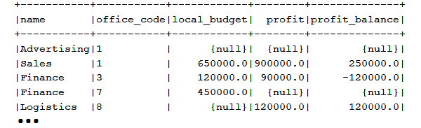
Figure 13.1 – Output

More examples are available in the Functions bundled code.

IIF()

The IIF() function implements the if-then-else logic via three arguments, as follows (this acts as the NVL2() function presented later):

IIF(boolean_expr, value_for_true_case, value_for_false_case)

It evaluates the first argument (boolean_expr) and returns the second argument (value_for_true_case) and third one (value_for_false_case), respectively.

For instance, the following usage of the jOOQ iif() function evaluates the DEPARTMENT.LOCAL_BUDGET.isNull() expression and outputs the text NO BUDGET or HAS BUDGET:

ctx.select(DEPARTMENT.DEPARTMENT_ID, DEPARTMENT.NAME,

      iif(DEPARTMENT.LOCAL_BUDGET.isNull(), 

        "NO BUDGET", "HAS BUDGET").as("budget"))

   .from(DEPARTMENT).fetch();

More examples, including imbricated IIF() usage, are available in the bundled code.

NULLIF()

The NULLIF(expr1, expr2) function returns NULL if the arguments are equal. Otherwise, it returns the first argument (expr1).

For instance, in legacy databases, it is a common practice to have a mixture of NULL and empty strings for missing values. We have intentionally created such a case in the OFFICE table for OFFICE.COUNTRY.

Since empty strings are not NULL values, using ISNULL() will not return them even if, for us, NULL values and empty strings may have the same mining. Using the jOOQ nullif() method is a handy approach for finding all missing data (NULL values and empty strings), as follows:

ctx.select(OFFICE.OFFICE_CODE, nullif(OFFICE.COUNTRY, ""))

    .from(OFFICE).fetch();

ctx.selectFrom(OFFICE)

    .where(nullif(OFFICE.COUNTRY, "").isNull()).fetch();

These examples are available in the Functions bundled code.

IFNULL() and ISNULL()

The IFNULL(expr1, expr2) and ISNULL(expr1, expr2) functions take two arguments and return the first one if it is not NULL. Otherwise, they return the second argument. The former is similar to Oracle's NVL() function presented later, while the latter is specific to SQL Server. Both of them are emulated by jOOQ via CASE expressions for all dialects that don't support them natively.

For instance, the following snippet of code produces 0 for each NULL value of DEPARTMENT.LOCAL_BUDGET via both jOOQ methods, ifnull() and isnull():

ctx.select(DEPARTMENT.DEPARTMENT_ID, DEPARTMENT.NAME,

      ifnull(DEPARTMENT.LOCAL_BUDGET, 0).as("budget_if"),

      isnull(DEPARTMENT.LOCAL_BUDGET, 0).as("budget_is"))

   .from(DEPARTMENT)

   .fetch();

Here is another example that fetches the customer's postal code or address:

ctx.select(

     ifnull(CUSTOMERDETAIL.POSTAL_CODE,  

       CUSTOMERDETAIL.ADDRESS_LINE_FIRST).as("address_if"),

     isnull(CUSTOMERDETAIL.POSTAL_CODE, 

       CUSTOMERDETAIL.ADDRESS_LINE_FIRST).as("address_is"))

  .from(CUSTOMERDETAIL).fetch();

More examples are available in the Functions bundled code.

NVL() and NVL2()

Some dialects (for example, Oracle) support two functions named NVL() and NVL2(). Both of them are emulated by jOOQ for all dialects that don't support them natively. The former acts like IFNULL(), while the latter acts like IIF(). So, NVL(expr1, expr2) produces the first argument if it is not NULL; otherwise, it produces the second argument.

For instance, let's use the jOOQ nvl() method for applying the variance formula used in finance to calculate the difference between a forecast and an actual result for DEPARTMENT.FORECAST_PROFIT and DEPARTMENT.PROFIT as ((ACTUAL PROFIT ÷ FORECAST PROFIT) - 1) * 100, as follows:

ctx.select(DEPARTMENT.NAME, ...,                

       round((nvl(DEPARTMENT.PROFIT, 0d).divide(

       nvl(DEPARTMENT.FORECAST_PROFIT, 10000d)))

       .minus(1d).mul(100), 2).concat("%").as("nvl"))

   .from(DEPARTMENT)

   .fetch();

If PROFIT is NULL, then we replace it with 0, and if FORECAST_PROFIT is NULL, then we replace it with a default profit of 10,000. Challenge yourself to write this query via ISNULL() as well.

On the other hand, NVL2(expr1, expr2, expr3) evaluates the first argument (expr1). If expr1 is not NULL, then it returns the second argument (expr2); otherwise, it returns the third argument (expr3).

For instance, each EMPLOYEE has a salary and an optional COMMISSION (a missing commission is NULL). Let's fetch salary + commission via jOOQ nvl2() and iif(), as follows:

ctx.select(EMPLOYEE.FIRST_NAME, EMPLOYEE.LAST_NAME,

 iif(EMPLOYEE.COMMISSION.isNull(),EMPLOYEE.SALARY,  

  EMPLOYEE.SALARY.plus(EMPLOYEE.COMMISSION))

    .as("iif1"),

 iif(EMPLOYEE.COMMISSION.isNotNull(),

  EMPLOYEE.SALARY.plus(EMPLOYEE.COMMISSION), EMPLOYEE.SALARY)

   .as("iif2"),

 nvl2(EMPLOYEE.COMMISSION,

  EMPLOYEE.SALARY.plus(EMPLOYEE.COMMISSION), EMPLOYEE.SALARY)

   .as("nvl2"))

 .from(EMPLOYEE)

 .fetch();

All three columns—iif1, iif2, and nvl2—should contain the same data. Regrettably, NVL can perform better than COALESCE in some Oracle cases. For more details, consider reading this article: https://connor-mcdonald.com/2018/02/13/nvl-vs-coalesce/. You can check out all the examples from this section in the Functions bundled code. Next, let's talk about numeric functions.

Numeric functions

jOOQ supports a comprehensive list of numeric functions, including ABS(), SIN(), COS(), EXP(), FLOOR(), GREATEST(), LEAST(), LN(), POWER(), SIGN(), SQRT(), and much more. Mainly, jOOQ exposes a set of methods that mirrors the names of these SQL functions and supports the proper number and type of arguments.

Since you can find all these functions listed and exemplified in the jOOQ manual, let's try here two examples of combining several of them to accomplish a common goal. For instance, a famous formula for computing the Fibonacci number is the Binet formula (notice that no recursion is required!):

Fib(n) = (1.6180339^n – (–0.6180339)^n) / 2.236067977

Writing this formula in jOOQ/SQL requires us to use the power() numeric function as follows (n is the number to compute):

ctx.fetchValue(round((power(1.6180339, n).minus(

      power(-0.6180339, n))).divide(2.236067977), 0));

How about computing the distance between two points expressed as (latitude1, longitude1), respectively (latitude2, longitude2)? Of course, exactly as in the case of the Fibonacci number, such computations are commonly done outside the database (directly in Java) or in a UDF or stored procedure, but trying to solve them in a SELECT statement is a good opportunity to quickly practice some numeric functions and get familiar with jOOQ syntax. So, here we go with the required math:

a = POWER(SIN((latitude2 − latitude1) / 2.0)), 2)

  + COS(latitude1) * COS(latitude2) 

      * POWER (SIN((longitude2 − longitude1) / 2.0), 2);

result = (6371.0 * (2.0 * ATN2(SQRT(a),SQRT(1.0 − a))));

This time, we need the jOOQ power(), sin(), cos(), atn2(), and sqrt() numeric methods, as shown here:

double pi180 = Math.PI / 180;

Field<BigDecimal> a = (power(sin(val((latitude2 - latitude1) 

 * pi180).divide(2d)), 2d).plus(cos(latitude1 * pi180)

   .mul(cos(latitude2 * pi180)).mul(power(sin(val((

     longitude2 - longitude1) * pi180).divide(2d)), 2d))));

ctx.fetchValue(inline(6371d).mul(inline(2d)

   .mul(atan2(sqrt(a), sqrt(inline(1d).minus(a))))));

You can practice these examples in the Functions bundled code.

String functions

Exactly as in case of SQL numeric functions, jOOQ supports an impressive set of SQL string functions, including ASCII(), CONCAT(), OVERLAY(), LOWER(), UPPER(), LTRIM(), RTRIM(), and so on. You can find each of them exemplified in the jOOQ manual, so here, let's try to use several string functions to obtain an output, as in this screenshot:

Figure 13.2 – Applying several SQL string functions

Transforming what we have in what we want can be expressed in jOOQ via several methods, including concat(), upper(), space(), substring(), lower(), and rpad()—of course, you can optimize or write the following query in different ways:

ctx.select(concat(upper(EMPLOYEE.FIRST_NAME), space(1),

         substring(EMPLOYEE.LAST_NAME, 1, 1).concat(". ("),

           lower(EMPLOYEE.JOB_TITLE),

              rpad(val(")"), 4, '.')).as("employee"))

   .from(EMPLOYEE)

   .fetch();

You can check out this example next to several examples of splitting a string by a delimiter in the Functions bundled code.

Date-time functions

The last category of functions covered in this section includes date-time functions. Mainly, jOOQ exposes a wide range of date-time functions that can be roughly categorized as functions that operate with java.sql.Date, java.sql.Time, and java.sql.Timestamp, and functions that operate with Java 8 date-time, java.time.LocalDate, java.time.LocalDateTime, and java.time.OffsetTime. jOOQ can't use the java.time.Duration or Period classes as they work differently from standard SQL intervals, though of course, converters and bindings can be applied.

Moreover, jOOQ comes with a substitute for JDBC missing java.sql.Interval data type, named org.jooq.types.Interval, having three implementations as DayToSecond, YearToMonth, and YearToSecond.

Here are a few examples that are pretty simple and intuitive. This first example fetches the current date as java.sql.Date and java.time.LocalDate:

Date r = ctx.fetchValue(currentDate());

LocalDate r = ctx.fetchValue(currentLocalDate());

This next example converts an ISO 8601 DATE string literal into a java.sql.Date data type:

Date r = ctx.fetchValue(date("2024-01-29"));

Adding an interval of 10 days to a Date and a LocalDate can be done like this:

var r = ctx.fetchValue(

 dateAdd(Date.valueOf("2022-02-03"), 10).as("after_10_days"));

var r = ctx.fetchValue(localDateAdd(

 LocalDate.parse("2022-02-03"), 10).as("after_10_days"));

Or, adding an interval of 3 months can be done like this:

var r = ctx.fetchValue(dateAdd(Date.valueOf("2022-02-03"), 

  new YearToMonth(0, 3)).as("after_3_month"));

Extracting the day of week (1 = Sunday, 2 = Monday, ..., 7 = Saturday) via the SQL EXTRACT() and jOOQ dayOfWeek() functions can be done like this:

int r = ctx.fetchValue(dayOfWeek(Date.valueOf("2021-05-06")));

int r = ctx.fetchValue(extract(

  Date.valueOf("2021-05-06"), DatePart.DAY_OF_WEEK));

You can check out more examples in the Functions bundled code. In the next section, let's tackle aggregate functions.

Aggregate functions

The most common aggregate functions (in an arbitrary order) are AVG(), COUNT(), MAX(), MIN(), and SUM(), including their DISTINCT variants. I'm pretty sure that you are very familiar with these aggregates and you've used them in many of your queries. For instance, here are two SELECT statements that compute the popular harmonic and geometric means for sales grouped by fiscal year. Here, we use the jOOQ sum() and avg() functions:

// Harmonic mean: n / SUM(1/xi), i=1…n

ctx.select(SALE.FISCAL_YEAR, count().divide(

     sum(inline(1d).divide(SALE.SALE_))).as("harmonic_mean"))

   .from(SALE).groupBy(SALE.FISCAL_YEAR).fetch();

And here, we compute the geometric mean:

// Geometric mean: EXP(AVG(LN(n)))

ctx.select(SALE.FISCAL_YEAR, exp(avg(ln(SALE.SALE_)))

            .as("geometric_mean"))

   .from(SALE).groupBy(SALE.FISCAL_YEAR).fetch();

But as you know (or as you'll find out shortly), there are many other aggregates that have the same goal of performing some calculations across a set of rows and returning a single output row. Again, jOOQ exposes dedicated methods whose names mirror the aggregates' names or represent suggestive shortcuts.

Next, let's see several aggregate functions that are less popular and are commonly used in statistics, finance, science, and other fields. One of them is dedicated to computing Standard Deviation, (https://en.wikipedia.org/wiki/Standard_deviation). In jOOQ, we have stddevSamp() for Sample and stddevPop() for Population. Here is an example of computing SSD, PSD, and emulation of PSD via population variance (introduced next) for sales grouped by fiscal year:

ctx.select(SALE.FISCAL_YEAR,

    stddevSamp(SALE.SALE_).as("samp"),   // SSD 

    stddevPop(SALE.SALE_).as("pop1"),    // PSD

    sqrt(varPop(SALE.SALE_)).as("pop2")) // PSD emulation

 .from(SALE).groupBy(SALE.FISCAL_YEAR).fetch();

Both SSD and PSD are supported in MySQL, PostgreSQL, SQL Server, Oracle, and many other dialects and are useful in different kinds of problems, from finance, statistics, forecasting, and so on. For instance, in statistics, we have the standard score (or so-called z-score) that represents the number of SDs placed above or below the population mean for a certain observation and having the formula z = (x - µ) / σ (z is z-score, x is the observation, µ is the mean, and σ is the SD). You can read further information on this here: https://en.wikipedia.org/wiki/Standard_score.

Now, considering that we store the number of sales (DAILY_ACTIVITY.SALES) and visitors (DAILY_ACTIVITY.VISITORS) in DAILY_ACTIVITY and we want to get some information about this data, since there is no direct comparison between sales and visitors, we have to come up with some meaningful representation, and this can be provided by z-scores. By relying on Common Table Expressions (CTEs) and SD, we can express in jOOQ the following query (of course, in production, using a stored procedure may be a better choice for such queries):

ctx.with("sales_stats").as(

      select(avg(DAILY_ACTIVITY.SALES).as("mean"),

        stddevSamp(DAILY_ACTIVITY.SALES).as("sd"))

      .from(DAILY_ACTIVITY))

   .with("visitors_stats").as(

      select(avg(DAILY_ACTIVITY.VISITORS).as("mean"),

        stddevSamp(DAILY_ACTIVITY.VISITORS).as("sd"))

      .from(DAILY_ACTIVITY))

   .select(DAILY_ACTIVITY.DAY_DATE,

     abs(DAILY_ACTIVITY.SALES

     .minus(field(name("sales_stats", "mean"))))

     .divide(field(name("sales_stats", "sd"), Float.class))

     .as("z_score_sales"),

      abs(DAILY_ACTIVITY.VISITORS

     .minus(field(name("visitors_stats", "mean"))))

     .divide(field(name("visitors_stats", "sd"), Float.class))

        .as("z_score_visitors"))

   .from(table("sales_stats"), 

     table("visitors_stats"), DAILY_ACTIVITY).fetch();

Among the results produced by this query, we remark the z-score of sales on 2004-01-06, which is 2.00. In the context of z-score analysis, this output is definitely worth a deeper investigation (typically, z-scores > 1.96 or < -1.96 are considered outliers that should be further investigated). Of course, this is not our goal, so let's jump to another aggregate.

Going further through statistical aggregates, we have variance, which is defined as the average of the squared differences from the mean or the average squared deviations from the mean (https://en.wikipedia.org/wiki/Variance). In jOOQ, we have sample variance via varSamp() and population variance via varPop(), as illustrated in this code example:

Field<BigDecimal> x = PRODUCT.BUY_PRICE;

ctx.select(varSamp(x)) // Sample Variance

    .from(PRODUCT).fetch();

ctx.select(varPop(x)) // Population Variance

    .from(PRODUCT).fetch();

Both of them are supported in MySQL, PostgreSQL, SQL Server, Oracle, and many other dialects, but just for fun, you can emulate sample variance via the COUNT() and SUM() aggregates as has been done in the following code snippet—just another opportunity to practice these aggregates:

ctx.select((count().mul(sum(x.mul(x)))

      .minus(sum(x).mul(sum(x)))).divide(count()

      .mul(count().minus(1))).as("VAR_SAMP"))

   .from(PRODUCT).fetch();

Next, we have linear regression (or correlation) functions applied for determining regression relationships between the dependent (denoted as Y) and independent (denoted as X) variable expressions (https://en.wikipedia.org/wiki/Regression_analysis). In jOOQ, we have regrSXX(),regrSXY(), regrSYY(), regrAvgX(), regrAvgXY(), regrCount(), regrIntercept(), regrR2(), and regrSlope().

For instance, in the case of regrSXY(y, x), y is the dependent variable expression and x is the independent variable expression. If y is PRODUCT.BUY_PRICE and x is PRODUCT.MSRP, then the linear regression per PRODUCT_LINE looks like this:

ctx.select(PRODUCT.PRODUCT_LINE,

    (regrSXY(PRODUCT.BUY_PRICE, PRODUCT.MSRP)).as("regr_sxy"))

    .from(PRODUCT).groupBy(PRODUCT.PRODUCT_LINE).fetch();

The functions listed earlier (including regrSXY()) are supported in all dialects, but they can be easily emulated as well. For instance, regrSXY() can be emulated as (SUM(X*Y)-SUM(X) * SUM(Y)/COUNT(*)), as illustrated here:

ctx.select(PRODUCT.PRODUCT_LINE,

     sum(PRODUCT.BUY_PRICE.mul(PRODUCT.MSRP))

      .minus(sum(PRODUCT.BUY_PRICE).mul(sum(PRODUCT.MSRP)

      .divide(count()))).as("regr_sxy"))

   .from(PRODUCT).groupBy(PRODUCT.PRODUCT_LINE).fetch();

In addition, regrSXY() can also be emulated as SUM(1) * COVAR_POP(expr1, expr2), where COVAR_POP() represents the population covariance and SUM(1) is actually REGR_COUNT(expr1, expr2). You can see this example in the bundled code next to many other emulations for REGR_FOO() functions and an example of calculating y = slope * x – intercept via regrSlope() and regrIntercept(), linear regression coefficients, but also via sum(), avg(), and max().

After population covariance (https://en.wikipedia.org/wiki/Covariance), COVAR_POP(), we have sample covariance, COVAR_SAMP(), which can be called like this:

ctx.select(PRODUCT.PRODUCT_LINE,

  covarSamp(PRODUCT.BUY_PRICE, PRODUCT.MSRP).as("covar_samp"),     

  covarPop(PRODUCT.BUY_PRICE, PRODUCT.MSRP).as("covar_pop")) 

   .from(PRODUCT)

   .groupBy(PRODUCT.PRODUCT_LINE)

   .fetch();

If your database doesn't support the covariance functions (for instance, MySQL or SQL Server), then you can emulate them via common aggregates—COVAR_SAMP() as (SUM(x*y) - SUM(x) * SUM(y) / COUNT(*)) / (COUNT(*) - 1), and COVAR_POP() as (SUM(x*y) - SUM(x) * SUM(y) / COUNT(*)) / COUNT(*). You can find examples in the AggregateFunctions bundled code.

An interesting function that is not supported by most databases (Exasol is one of the exceptions) but is provided by jOOQ is the synthetic product() function. This function represents multiplicative aggregation emulated via exp(sum(log(arg))) for positive numbers, and it performs some extra work for zero and negative numbers. For instance, in finance, there is an index named Compounded Month Growth Rate (CMGR) that is computed based on monthly revenue growth, as we have in SALE.REVENUE_GROWTH. The formula is (PRODUCT (1 + SALE.REVENUE_GROWTH))) ^ (1 / COUNT()), and we've applied it for each year here:

ctx.select(SALE.FISCAL_YEAR,

      round((product(one().plus(

         SALE.REVENUE_GROWTH.divide(100)))

            .power(one().divide(count()))).mul(100) ,2)

               .concat("%").as("CMGR"))

   .from(SALE).groupBy(SALE.FISCAL_YEAR).fetch();

We also multiply everything by 100 to obtain the result as a percent. You can find this example in the AggregateFunctions bundled code, next to other aggregation functions such as BOOL_AND(), EVERY(), BOOL_OR(), and functions for bitwise operations.

When you have to use an aggregate function that is partially supported or not supported by jOOQ, you can rely on the aggregate()/ aggregateDistinct() methods. Of course, your database must support the called aggregate function. For instance, jOOQ doesn't support the Oracle APPROX_COUNT_DISTINCT() aggregation function, which represents an alternative to the COUNT (DISTINCT expr) function. This is useful for approximating the number of distinct values while processing large amounts of data significantly faster than the traditional COUNT function, with negligible deviation from the exact number. Here is a usage of the (String name, Class<T> type, Field<?>... arguments) aggregate, which is just one of the provided flavors (check out the documentation for more):

ctx.select(ORDERDETAIL.PRODUCT_ID, 

     aggregate("approx_count_distinct", Long.class,  

       ORDERDETAIL.ORDER_LINE_NUMBER).as("approx_count"))  

   .from(ORDERDETAIL)

   .groupBy(ORDERDETAIL.PRODUCT_ID)

   .fetch();   

You can find this example in the AggregateFunctions bundled code for Oracle.

Window functions

Window functions are extremely useful and powerful; therefore, they represent a must-know topic for every developer that interacts with a database via SQL. In a nutshell, the best way to quickly overview window functions is to start from a famous diagram representing a comparison between an aggregation function and a window function that highlights the main difference between them, as represented here:

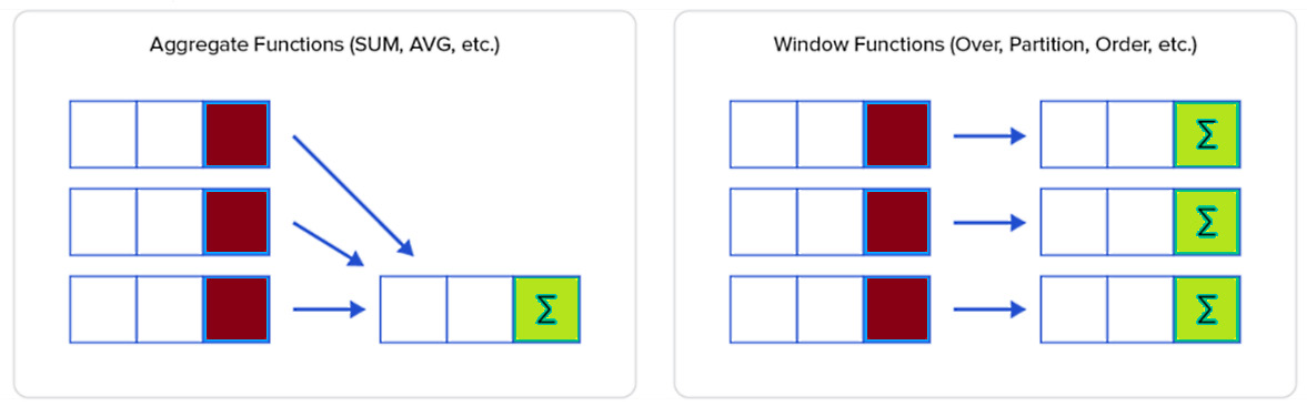
Figure 13.3 – Aggregate functions versus window functions

As you can see, both the aggregate function and the window function calculate something on a set of rows, but a window function doesn't aggregate or group these rows into a single output row. A window function relies on the following syntax:

window_function_name (expression) OVER (

    Partition Order Frame

)

This syntax can be explained as follows:

Obviously, window_function_name represents the window function name, such as ROW_NUMBER(), RANK(), and so on.

expression identifies the column (or target expression) on which this window function will operate.

The OVER clause signals that this is a window function, and it consists of three clauses: Partition, Order, and Frame. By adding the OVER clause to any aggregate function, you transform it into a window function.

The Partition clause is optional, and its goal is to divide the rows into partitions. Next, the window function will operate on each partition. It has the following syntax: PARTITION BY expr1, expr2, .... If PARTITION BY is omitted, then the entire result set represents a single partition. To be entirely accurate, if PARTITION BY is omitted, then all the data produced by FROM/WHERE/GROUP BY/HAVING represents a single partition.

The Order clause is also optional, and it handles the order of rows in a partition. Its syntax is ORDER BY expression [ASC | DESC] [NULLS {FIRST| LAST}] ,....

The Frame clause demarcates a subset of the current partition. The common syntax is mode BETWEEN start_of_frame AND end_of_frame [frame_exclusion].

mode instructs the database about how to treat the input rows. Three possible values indicate the type of relationship between the frame rows and the current row: ROWS, GROUPS, and RANGE.

ROWS

The ROWS mode specifies that the offsets of the frame rows and the current row are row numbers (the database sees each input row as an individual unit of work). In this context, start_of_frame and end_of_frame determine which rows the window frame starts and ends with.

In this context, start_of_frame can be N PRECEDING, which means that the frame starts at nth rows before the currently evaluated row (in jOOQ, rowsPreceding(n)), UNBOUNDED PRECEDING, which means that the frame starts at the first row of the current partition (in jOOQ, rowsUnboundedPreceding()), and CURRENT ROW (jOOQ rowsCurrentRow()).

The end_of_frame value can be CURRENT ROW (previously described), N FOLLOWING, which means that the frame ends at the nth row after the currently evaluated row (in jOOQ, rowsFollowing(n)), and UNBOUNDED FOLLOWING, which means that the frame ends at the last row of the current partition (in jOOQ, rowsUnboundedFollowing()).

Check out the following diagram containing some examples:

Figure 13.4 – ROWS mode examples

What's in gray represents the included rows.

GROUPS

The GROUPS mode instructs the database that the rows with duplicate sorting values should be grouped together. So, GROUPS is useful when duplicate values are present.

In this context, start_of_frame and end_of_frame accept the same values as ROWS. But, in the case of start_of_frame, CURRENT_ROW points to the first row in a group that contains the current row, while in the case of end_of_frame, it points to the last row in a group that contains the current row. Moreover, N PRECEDING/FOLLOWING refers to groups that should be considered as the number of groups before, respectively, after the current group. On the other hand, UNBOUNDED PRECEDING/FOLLOWING has the same meaning as in the case of ROWS.

Check out the following diagram containing some examples:

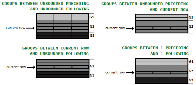
Figure 13.5 – GROUPS mode examples

There are three groups (G1, G2, and G3) represented in different shades of gray.

RANGE

The RANGE mode doesn't tie rows as ROWS/GROUPS. This mode works on a given range of values of the sorting column. This time, for start_of_frame and end_of_frame, we don't specify the number of rows/groups; instead, we specify the maximum difference of values that the window frame should contain. Both values must be expressed in the same units (or, meaning) as the sorting column is.

In this context, for start_of_frame,we have the following: (this time, N is a value in the same unit as the sorting column is) N PRECEDING (in jOOQ, rangePreceding(n)), UNBOUNDED PRECEDING (in jOOQ, rangeUnboundedPreceding()), and CURRENT ROW (in jOOQ, rangeCurrentRow()). For end_of_frame, we have CURRENT ROW, UNBOUNDED FOLLOWING (in jOOQ, rangeUnboundedFollowing()), N FOLLOWING (in jOOQ, rangeFollowing(n)).

Check out the following diagram containing some examples:

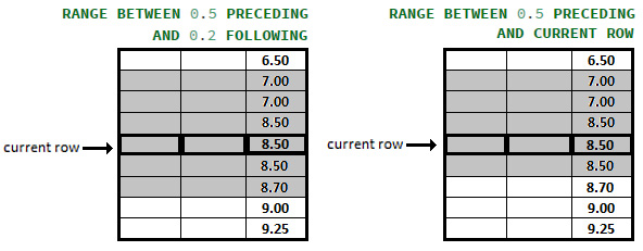
Figure 13.6 – RANGE mode examples

What's in gray represents the included rows.

BETWEEN start_of_frame AND end_of_frame

Especially for the BETWEEN start_of_frame AND end_of_frame construction, jOOQ comes with fooBetweenCurrentRow(), fooBetweenFollowing(n), fooBetweenPreceding(n), fooBetweenUnboundedFollowing(), and fooBetweenUnboundedPreceding(). In all these methods, foo can be replaced with rows, groups, or range.

In addition, for creating compound frames, jOOQ provides andCurrentRow(), andFollowing(n), andPreceding(n), andUnboundedFollowing(), and andUnboundedPreceding().

frame_exclusion

Via the frame_exclusion optional part, we can exclude certain rows from the window frame. frame_exclusion works exactly the same for all three modes. Possible values are listed here:

• EXCLUDE CURRENT ROW—Exclude the current row (in jOOQ, excludeCurrentRow()).
• EXCLUDE GROUP—Exclude the current row but also exclude all peer rows (for instance, exclude all rows having the same value in the sorting column). In jOOQ, we have the excludeGroup() method.
• EXCLUDE TIES—Exclude all peer rows, but not the current row (in jOOQ, excludeTies()).
• EXCLUDE NO OTHERS—This is the default, and it means to exclude nothing (in jOOQ, excludeNoOthers()).

To better visualize these options, check out the following diagram:

Figure 13.7 – Examples of excluding rows

Speaking about the logical order of operations in SQL, we notice here that window functions are placed between HAVING and SELECT:

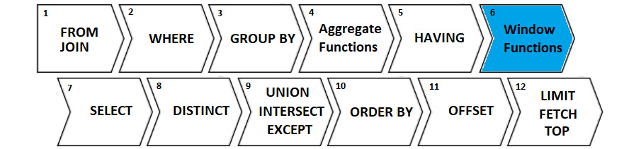
Figure 13.8 – Logical order of operations in SQL

Also, I think is useful to explain that window functions can act upon data produced by all the previous steps 1-5, and can be declared in all the following steps 7-12 (effectively only in 7 and 10). Before jumping into some window functions examples, let's quickly cover a less-known but quite useful SQL clause.

The QUALIFY clause

Some databases (for instance, Snowflake) support a clause named QUALIFY. Via this clause, we can filter (apply a predicate) the results of window functions. Mainly, a SELECT … QUALIFY clause is evaluated after window functions are computed, so after Window Functions (Step 6 in Figure 13.8) and before DISTINCT (Step 8 in Figure 13.8). The syntax of QUALIFY is QUALIFY <predicate>, and in the following screenshot, you can see how it makes the difference (this query returns every 10th product from the PRODUCT table via the ROW_NUMBER() window function):

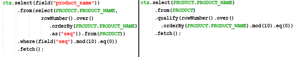
Figure 13.9 – Logical order of operations in SQL

By using the QUALIFY clause, we eliminate the subquery and the code is less verbose. Even if this clause has poor native support among database vendors, jOOQ emulates it for all the supported dialects. Cool, right?! During this chapter, you'll see more examples of using the QUALIFY clause.

Working with ROW_NUMBER()

ROW_NUMBER() is a ranking window function that assigns a sequential number to each row (it starts from 1). A simple example is shown here:

Figure 13.10 – Simple example of ROW_NUMBER()

You already saw an example of paginating database views via ROW_NUMBER() in Chapter 12, Pagination and Dynamic Queries, so you should have no problem understanding the next two examples.

Let's assume that we want to compute the median (https://en.wikipedia.org/wiki/Median) of PRODUCT.QUANTITY_IN_STOCK. In Oracle and PostgreSQL, this can be done via the built-in median() aggregate function, but in MySQL and SQL Server, we have to emulate it somehow, and a good approach consists of using ROW_NUMBER(), as follows:

Field<Integer> x = PRODUCT.QUANTITY_IN_STOCK.as("x");

Field<Double> y = inline(2.0d).mul(rowNumber().over()

   .orderBy(PRODUCT.QUANTITY_IN_STOCK))

   .minus(count().over()).as("y");

ctx.select(avg(x).as("median")).from(select(x, y)

   .from(PRODUCT))

   .where(y.between(0d, 2d))

   .fetch();

That was easy! Next, let's try to solve a different kind of problem, and let's focus on the ORDER table. Each order has a REQUIRED_DATE and STATUS value as Shipped, Cancelled, and so on. Let's assume that we want to see the clusters (also known as islands) represented by continuous periods of time where the score (STATUS, in this case) stayed the same. An output sample can be seen here:

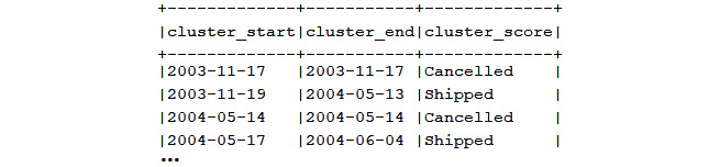
Figure 13.11 – Clusters

If we have a requirement to solve this problem via ROW_NUMBER() and to express it in jOOQ, then we may come up with this query:

Table<?> t = select(

  ORDER.REQUIRED_DATE.as("rdate"), ORDER.STATUS.as("status"),

  (rowNumber().over().orderBy(ORDER.REQUIRED_DATE)

    .minus(rowNumber().over().partitionBy(ORDER.STATUS)

  .orderBy(ORDER.REQUIRED_DATE))).as("cluster_nr"))

  .from(ORDER).asTable("t");

ctx.select(min(t.field("rdate")).as("cluster_start"),

           max(t.field("rdate")).as("cluster_end"),

           min(t.field("status")).as("cluster_score"))

   .from(t)

   .groupBy(t.field("cluster_nr"))

   .orderBy(1)

   .fetch();

You can practice these examples in the RowNumber bundled code.

Working with RANK()

RANK() is a ranking window function that assigns a rank to each row within the partition of a result set. The rank of a row is computed as 1 + the number of ranks before it. The columns having the same values get the same ranks; therefore, if multiple rows have the same rank, then the rank of the next row is not consecutive. Think of a competition where two athletes share the first place (or the gold medal) and there is no second place (so, no silver medal). A simple example is provided here:

Figure 13.12 – Simple example of RANK()

Here is another example that ranks ORDER by year and months of ORDER.ORDER_DATE:

ctx.select(ORDER.ORDER_ID, ORDER.CUSTOMER_NUMBER, 

      ORDER.ORDER_DATE, rank().over().orderBy(

        year(ORDER.ORDER_DATE), month(ORDER.ORDER_DATE))) 

   .from(ORDER).fetch();

The year() and month() shortcuts are provided by jOOQ to avoid the usage of the SQL EXTRACT() function. For instance, year(ORDER.ORDER_DATE) can be written as extract(ORDER.ORDER_DATE, DatePart.YEAR) as well.

How about ranking YEAR is the partition? This can be expressed in jOOQ like this:

ctx.select(SALE.EMPLOYEE_NUMBER, SALE.FISCAL_YEAR,  

  sum(SALE.SALE_), rank().over().partitionBy(SALE.FISCAL_YEAR)

     .orderBy(sum(SALE.SALE_).desc()).as("sale_rank"))

   .from(SALE)

   .groupBy(SALE.EMPLOYEE_NUMBER, SALE.FISCAL_YEAR)

   .fetch();

Finally, let's see an example that ranks the products. Since a partition can be defined via multiple columns, we can easily rank the products by PRODUCT_VENDOR and PRODUCT_SCALE, as shown here:

ctx.select(PRODUCT.PRODUCT_NAME, PRODUCT.PRODUCT_VENDOR, 

    PRODUCT.PRODUCT_SCALE, rank().over().partitionBy(

      PRODUCT.PRODUCT_VENDOR, PRODUCT.PRODUCT_SCALE)

   .orderBy(PRODUCT.PRODUCT_NAME))

   .from(PRODUCT)

   .fetch();

You can practice these examples and more in Rank.

Working with DENSE_RANK()

DENSE_RANK() is a window function that assigns a rank to each row within a partition or result set with no gaps in ranking values. A simple example is shown here:

Figure 13.13 – Simple example of DENSE_RANK()

In Chapter 12, Pagination and Dynamic Queries, you already saw an example of using DENSE_RANK() for paginating JOIN statements. Next, let's have another case of ranking employees (EMPLOYEE) in offices (OFFICE) by their salary (EMPLOYEE.SALARY), as follows:

ctx.select(EMPLOYEE.FIRST_NAME, EMPLOYEE.LAST_NAME, 

  EMPLOYEE.SALARY, OFFICE.CITY, OFFICE.COUNTRY,       

  OFFICE.OFFICE_CODE, denseRank().over().partitionBy(

    OFFICE.OFFICE_CODE).orderBy(EMPLOYEE.SALARY.desc())

      .as("salary_rank"))

   .from(EMPLOYEE)

   .innerJoin(OFFICE)

   .on(OFFICE.OFFICE_CODE.eq(EMPLOYEE.OFFICE_CODE)).fetch();

An output fragment looks like this (notice that the employees having the same salary get the same rank):

Figure 13.14 – Output

Finally, let's use DENSE_RANK() for selecting the highest salary from each office, including duplicates. This time, let's use the QUALIFY clause as well. The code is illustrated in the following snippet:

select(EMPLOYEE.FIRST_NAME, EMPLOYEE.LAST_NAME, 

    EMPLOYEE.SALARY, OFFICE.CITY, OFFICE.COUNTRY,   

    OFFICE.OFFICE_CODE)

 .from(EMPLOYEE)

 .innerJoin(OFFICE)

  .on(OFFICE.OFFICE_CODE.eq(EMPLOYEE.OFFICE_CODE))

 .qualify(denseRank().over().partitionBy(OFFICE.OFFICE_CODE)

   .orderBy(EMPLOYEE.SALARY.desc()).eq(1))

 .fetch();

Before going further, here is a nice read: https://blog.jooq.org/2014/08/12/the-difference-between-row_number-rank-and-dense_rank/. You can check out these examples in the DenseRank bundled code.

Working with PERCENT_RANK()

The PERCENT_RANK() window function calculates the percentile rankings ((rank - 1) / (total_rows - 1)) of rows in a result set and returns a value between 0 exclusive and 1 inclusive. The first row in the result set always has the percent rank equal to 0. This function doesn't count NULL values and is nondeterministic. Usually, the final result is multiplied by 100 to express as a percentage.

The best way to understand this function is via an example. Let's assume that we want to compute the percentile rank for employees in each office by their salaries. The query expressed in jOOQ will look like this:

ctx.select(EMPLOYEE.FIRST_NAME, EMPLOYEE.LAST_NAME, 

   EMPLOYEE.SALARY, OFFICE.OFFICE_CODE, OFFICE.CITY,    

   OFFICE.COUNTRY, round(percentRank().over()

      .partitionBy(OFFICE.OFFICE_CODE)

      .orderBy(EMPLOYEE.SALARY).mul(100), 2)

      .concat("%").as("PERCENTILE_RANK"))

   .from(EMPLOYEE)

   .innerJoin(OFFICE)

   .on(EMPLOYEE.OFFICE_CODE.eq(OFFICE.OFFICE_CODE))

   .fetch();

The following screenshot represents a snippet of the result:

Figure 13.15 – Percent rank output

So, how do we interpret this output? A percentile rank is commonly defined as the proportion of results (or scores) in a distribution that a certain result (or score) is greater than or equal to (sometimes only greater than counts). For example, if you get a result/score of 90 on a certain test and this result/score was greater than (or equal to) the results/scores of 75% of the participants taking the test, then your percentile rank is 75. You would be in the 75th percentile.

In other words, in office 1, we can say that 40% of employees have salaries lower than Anthony Bow (check the third row), so Anthony Bow is in the 40th percentile. Also, in office 1, Diane Murphy has the highest salary since 100% of employees have salaries lower than her salary (check the sixth row). When the current row is the first in the partition then there is no previous data to consider, therefore the percentile rank is 0. An interesting case is George Vanauf (last row) having a percentile rank of 0%. Because his salary ($55,000) is equal to the salary of Foon Yue Tseng, we can say that nobody has a salary lower than his.

A common use case for PERCENT_RANK() is to categorize data into custom groups (also known as custom binning). For example, let's consider that we want to count departments having a low (smaller than the 20th percentile), medium (between the 20th and 80th percentile), and high (greater than 80th percentile) profit. Here's the code we'd use to calculate this:

ctx.select(count().filterWhere(field("p").lt(0.2))

     .as("low_profit"),

  count().filterWhere(field("p").between(0.2, 0.8))

     .as("good_profit"),

  count().filterWhere(field("p").gt(0.8))

     .as("high_profit"))

 .from(select(percentRank().over()

        .orderBy(DEPARTMENT.PROFIT).as("p"))

        .from(DEPARTMENT)

        .where(DEPARTMENT.PROFIT.isNotNull()))     

 .fetch();

You can practice these examples—and more—in the PercentRank bundled code.

Working with CUME_DIST()

CUME_DIST() is a window function that computes the cumulative distribution of a value within a set of values. In other words, CUME_DIST() divides the number of rows having values less than or equal to the current row's value by the total number of rows. The returned value is greater than zero and less than or equal to one (0 < CUME_DIST() <= 1). The columns having repeated values get the same CUME_DIST() value. A simple example is provided here:

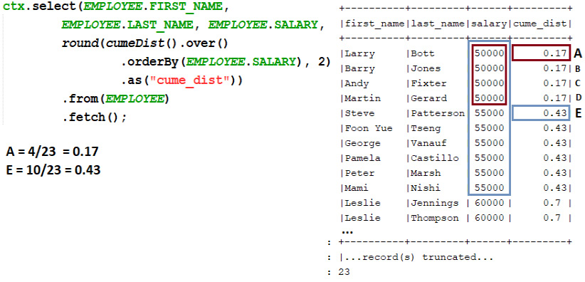
Figure 13.16 – Simple example of CUME_DIST()

So, we have a result set of 23 rows. For the first row (denoted as A), CUME_DIST() finds the number of rows having a value less than or equal to 50000. The result is 4. Then, the function divides 4 by the total number of rows, which is 23: 4/23. The result is 0.17 or 17%. The same logic is applied to the next rows.

How about fetching the top 25% of sales in 2003 and 2004? This can be solved via CUME_DIST() and the handy QUALIFY clause, as follows:

ctx.select(concat(EMPLOYEE.FIRST_NAME, inline(" "), 

 EMPLOYEE.LAST_NAME).as("name"), SALE.SALE_, SALE.FISCAL_YEAR)

   .from(EMPLOYEE)

   .join(SALE)

   .on(EMPLOYEE.EMPLOYEE_NUMBER.eq(SALE.EMPLOYEE_NUMBER)

    .and(SALE.FISCAL_YEAR.in(2003, 2004)))

   .qualify(cumeDist().over().partitionBy(SALE.FISCAL_YEAR)

   .orderBy(SALE.SALE_.desc()).lt(BigDecimal.valueOf(0.25)))

   .fetch();

You can practice these examples in the CumeDist bundled code.

Working with LEAD()/LAG()

LEAD() is a window function that looks forward a specified number of rows (offset, by default 1) and accesses that row from the current row. LAG() works the same as LEAD(), but it looks back. For both, we can optionally specify a default value to be returned when there is no subsequent row (LEAD()) or there is no preceding row (LAG()) instead of returning NULL. A simple example is provided here:

Figure 13.17 – Simple example of LEAD() and LAG()

Besides the lead/lag(Field<T> field) syntax used in this example, jOOQ also exposes lead/lag(Field<T> field, int offset), lead/lag(Field<T> field, int offset, Field<T> defaultValue), and lead/lag(Field<T> field, int offset, T defaultValue). In this example, lead/lag(ORDER.ORDER_DATE) uses an offset of 1, so is the same thing as lead/lag(ORDER.ORDER_DATE, 1).

Here is an example that, for each employee, displays the salary and next salary using the office as a partition of LEAD(). When LEAD() reaches the end of the partition, we use 0 instead of NULL:

ctx.select(OFFICE.OFFICE_CODE, OFFICE.CITY, OFFICE.COUNTRY,

 EMPLOYEE.FIRST_NAME, EMPLOYEE.LAST_NAME, EMPLOYEE.SALARY,

 lead(EMPLOYEE.SALARY, 1, 0).over()

    .partitionBy(OFFICE.OFFICE_CODE)

      .orderBy(EMPLOYEE.SALARY).as("next_salary"))

   .from(OFFICE)

   .innerJoin(EMPLOYEE)

   .on(OFFICE.OFFICE_CODE.eq(EMPLOYEE.OFFICE_CODE))

   .fetch();

Next, let's tackle an example of calculating the Month-Over-Month (MOM) growth rate. This financial indicator is useful for benchmarking the business, and we already have it in the SALE.REVENUE_GROWTH column. But here is the query that can calculate it via the LAG() function for the year 2004:

ctx.select(SALE.FISCAL_MONTH,

  inline(100).mul((SALE.SALE_.minus(lag(SALE.SALE_, 1)

    .over().orderBy(SALE.FISCAL_MONTH)))

    .divide(lag(SALE.SALE_, 1).over()

     .orderBy(SALE.FISCAL_MONTH))).concat("%").as("MOM"))

   .from(SALE)

   .where(SALE.FISCAL_YEAR.eq(2004))

   .orderBy(SALE.FISCAL_MONTH)

   .fetch();

For more examples, including an example of funneling drop-off metrics and one about time-series analysis, please check out the LeadLag bundled code.

Working with NTILE()

NTILE(n) is a window function commonly used for distributing the number of rows in the specified n number of groups or buckets. Each bucket has a number (starting at 1) that indicates the bucket to which this row belongs. A simple example is provided here:

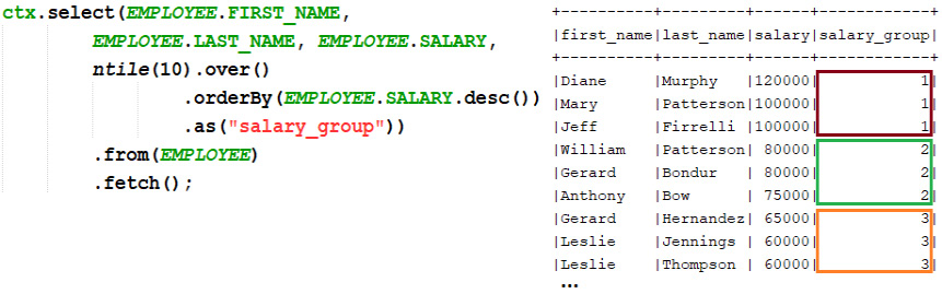
Figure 13.18 – Simple example of NTILE()

So, in this example, we've distributed EMPLOYEE.SALARY in 10 buckets. NTILE() strives to determine how many rows should be in each bucket in order to provide the number of buckets and to keep them approximately equal.

Among its use cases, NTILE() is useful for calculating Recency, Frequency, and Monetary (RFM) indices (https://en.wikipedia.org/wiki/RFM_(market_research)). In short, the RFM analysis is basically an indexing technique that relies on past purchase behavior to determine different segments of customers.

In our case, the past purchase behavior of each customer (ORDER.CUSTOMER_NUMBER) is stored in the ORDER table, especially in ORDER.ORDER_ID, ORDER.ORDER_DATE, and ORDER.AMOUNT.

Based on this information, we attempt to divide customers into four equal groups based on the distribution of values for R, F, and M. Four equal groups across RFM variables produce 43=64 potential segments. The result consists of a table having a score between 1 and 4 for each of the quantiles (R, F, and M). The query speaks for itself, as we can see here:

ctx.select(field("customer_number"),

    ntile(4).over().orderBy(field("last_order_date"))

     .as("rfm_recency"),

    ntile(4).over().orderBy(field("count_order"))

     .as("rfm_frequency"),

    ntile(4).over().orderBy(field("avg_amount"))

     .as("rfm_monetary")).from(

     select(ORDER.CUSTOMER_NUMBER.as("customer_number"),

      max(ORDER.ORDER_DATE).as("last_order_date"),

      count().as("count_order"),

      avg(ORDER.AMOUNT).as("avg_amount"))

        .from(ORDER)

        .groupBy(ORDER.CUSTOMER_NUMBER))

  .fetch();

A sample output is provided here:

Figure 13.19 – RFM sample

By combining the RFM result as R*100+F*10+M, we can obtain an aggregate score. This is available next to more examples in the Ntile bundled code.

Working with FIRST_VALUE() and LAST_VALUE()

FIRST_VALUE(expr) returns the value of the specified expression (expr) with respect to the first row in the window frame.

NTH_VALUE(expr, offset) returns the value of the specified expression (expr) with respect to the offset row in the window frame.

LAST_VALUE(expr) returns the value of the specified expression (expr) with respect to the last row in the window frame.

Let's assume that our goal is to obtain the cheapest and most expensive product per product line, as in the following screenshot:

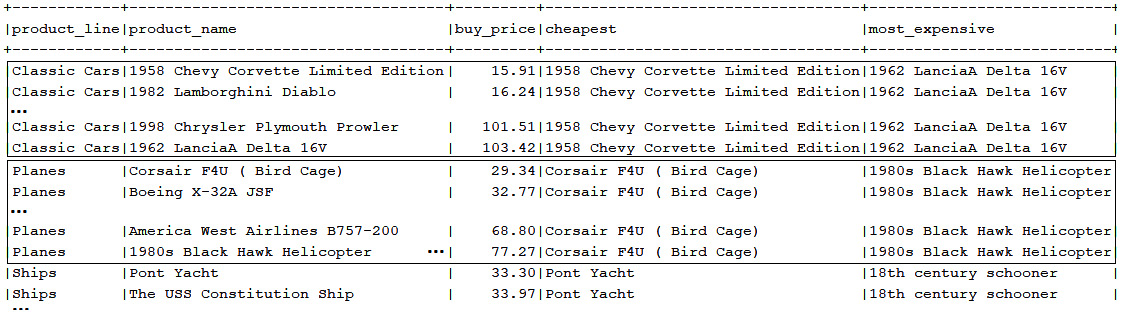
Figure 13.20 – Cheapest and most expensive product per product line

Accomplishing this task via FIRST_VALUE() and LAST_VALUE() can be done like this:

ctx.select(PRODUCT.PRODUCT_LINE, 

  PRODUCT.PRODUCT_NAME, PRODUCT.BUY_PRICE,

  firstValue(PRODUCT.PRODUCT_NAME).over()

   .partitionBy(PRODUCT.PRODUCT_LINE)

     .orderBy(PRODUCT.BUY_PRICE).as("cheapest"),

  lastValue(PRODUCT.PRODUCT_NAME).over()

   .partitionBy(PRODUCT.PRODUCT_LINE)

     .orderBy(PRODUCT.BUY_PRICE)

       .rangeBetweenUnboundedPreceding()

       .andUnboundedFollowing().as("most_expensive"))

  .from(PRODUCT)

  .fetch(); 

If the window frame is not specified, then the default window frame depends on the presence of ORDER BY. If ORDER BY is present, then the window frame is RANGE BETWEEN UNBOUNDED PRECEDING AND CURRENT ROW. If ORDER BY is not present, then the window frame is RANGE BETWEEN UNBOUNDED PRECEDING AND UNBOUNDED FOLLOWING.

Having this in mind, in our case, FIRST_VALUE() can rely on the default window frame to return the first row of the partition, which is the smallest price. On the other hand, LAST_VALUE() must explicitly define the window frame as RANGE BETWEEN UNBOUNDED PRECEDING AND UNBOUNDED FOLLOWING to return the highest price.

Here is another example of fetching the second most expensive product by product line via NTH_VALUE():

ctx.select(PRODUCT.PRODUCT_LINE, 

  PRODUCT.PRODUCT_NAME, PRODUCT.BUY_PRICE,

  nthValue(PRODUCT.PRODUCT_NAME, 2).over()

   .partitionBy(PRODUCT.PRODUCT_LINE)

    .orderBy(PRODUCT.BUY_PRICE.desc())

     .rangeBetweenUnboundedPreceding()

     .andUnboundedFollowing().as("second_most_expensive"))

   .from(PRODUCT)

   .fetch();

The preceding query orders BUY_PRICE in descending order for fetching the second most expensive product by product line. But this is mainly the second row from the bottom, therefore we can rely on the FROM LAST clause (in jOOQ, fromLast()) to express it, as follows:

ctx.select(PRODUCT.PRODUCT_LINE, 

   PRODUCT.PRODUCT_NAME, PRODUCT.BUY_PRICE,

   nthValue(PRODUCT.PRODUCT_NAME, 2).fromLast().over()

   .partitionBy(PRODUCT.PRODUCT_LINE)

    .orderBy(PRODUCT.BUY_PRICE)

     .rangeBetweenUnboundedPreceding()

     .andUnboundedFollowing().as("second_most_expensive"))

   .from(PRODUCT)

   .fetch();

This query works fine in Oracle, which supports FROM FIRST (fromFirst()), FROM LAST (fromLast()), IGNORE NULLS (ignoreNulls()), and RESPECT NULLS (respectNulls()).

You can practice these examples in the FirstLastNth bundled code.

Working with RATIO_TO_REPORT()

RATIO_TO_REPORT(expr) computes the ratio of the specified value to the sum of values in the set. If the given expr value is evaluated as null, then this function returns null. A simple example is provided here:

Figure 13.21 – Simple example of RATIO_TO_REPORT()

For instance, for the first row, the ratio is computed as 51241.54 / 369418.38, where 369418.38 is the sum of all sales. After applying the round() function, the result is 0.14 or 14%, but if we want to compute the ratio of the current sale per fiscal year, we can do it via PARTITION BY, as shown here:

ctx.select(SALE.EMPLOYEE_NUMBER, SALE.FISCAL_YEAR, SALE.SALE_,

  round(ratioToReport(SALE.SALE_).over()

          .partitionBy(SALE.FISCAL_YEAR), 2)

          .as("ratio_to_report_sale"))

  .from(SALE).fetch();

Let's compute the ratio of the current sum of salaries per employee and express it in percentages, like so:

ctx.select(OFFICE.OFFICE_CODE, 

     sum(EMPLOYEE.SALARY).as("salaries"),

       ratioToReport(sum(EMPLOYEE.SALARY)).over()

        .mul(100).concat("%").as("ratio_to_report"))

   .from(OFFICE)

   .join(EMPLOYEE)

   .on(OFFICE.OFFICE_CODE.eq(EMPLOYEE.OFFICE_CODE))

   .groupBy(OFFICE.OFFICE_CODE)

   .orderBy(OFFICE.OFFICE_CODE)

   .fetch();

You can check out these examples in the RatioToReport bundled code.

Aggregates as window functions

Aggregate functions can be used as window functions as well. For instance, let's use the SUM() aggregate function as a window function for computing the sum of the successfully transferred amount per customer until each caching date, as illustrated in the following screenshot:

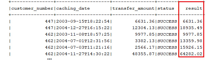
Figure 13.22 – Sum of the transferred amount until each caching date

The jOOQ query can be expressed like this:

ctx.select(BANK_TRANSACTION.CUSTOMER_NUMBER,   

  BANK_TRANSACTION.CACHING_DATE,

  BANK_TRANSACTION.TRANSFER_AMOUNT, BANK_TRANSACTION.STATUS,

  sum(BANK_TRANSACTION.TRANSFER_AMOUNT).over()

   .partitionBy(BANK_TRANSACTION.CUSTOMER_NUMBER)

   .orderBy(BANK_TRANSACTION.CACHING_DATE)

   .rowsBetweenUnboundedPreceding().andCurrentRow().as("result"))

  .from(BANK_TRANSACTION)

  .where(BANK_TRANSACTION.STATUS.eq("SUCCESS")).fetch();

Or, let's use the AVG() aggregate function as a window function for computing the average of prices for the preceding three ordered products on each order, as illustrated in the following screenshot:

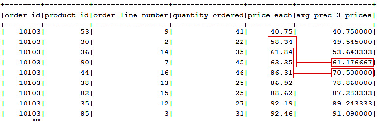
Figure 13.23 – Average of prices for the preceding three ordered products on each order

The query looks like this:

ctx.select(ORDERDETAIL.ORDER_ID, ORDERDETAIL.PRODUCT_ID, ...,

       avg(ORDERDETAIL.PRICE_EACH).over()

        .partitionBy(ORDERDETAIL.ORDER_ID)

        .orderBy(ORDERDETAIL.PRICE_EACH)

        .rowsPreceding(2).as("avg_prec_3_prices"))

   .from(ORDERDETAIL).fetch();

How about calculating a running average flavor—in other words, create a report that shows every transaction in March 2005 for Visa Electron cards? Additionally, this report shows the daily average transaction amount relying on a 3-day moving average. The code to accomplish this is shown in the following snippet:

ctx.select(

  BANK_TRANSACTION.CACHING_DATE, BANK_TRANSACTION.CARD_TYPE,

  sum(BANK_TRANSACTION.TRANSFER_AMOUNT).as("daily_sum"),

  avg(sum(BANK_TRANSACTION.TRANSFER_AMOUNT)).over()

    .orderBy(BANK_TRANSACTION.CACHING_DATE)

      .rowsBetweenPreceding(2).andCurrentRow()

         .as("transaction_running_average"))

   .from(BANK_TRANSACTION)

   .where(BANK_TRANSACTION.CACHING_DATE

   .between(LocalDateTime.of(2005, 3, 1, 0, 0, 0),

            LocalDateTime.of(2005, 3, 31, 0, 0, 0))

   .and(BANK_TRANSACTION.CARD_TYPE.eq("VisaElectron")))   

   .groupBy(BANK_TRANSACTION.CACHING_DATE, 

            BANK_TRANSACTION.CARD_TYPE)

   .orderBy(BANK_TRANSACTION.CACHING_DATE).fetch();

As Lukas Eder mentioned: "What's most mind-blowing about aggregate window functions is that even user-defined aggregate functions can be used as window functions!"

You can check out more examples (for instance, in the PostgreSQL bundled code, you can find queries for How many other employees have the same salary as me? and How many sales are better by 5,000 or less?) in the AggregateWindowFunctions bundled code.

Aggregate functions and ORDER BY

Certain aggregate functions output significantly different results depending on their input order. By default, this ordering is not specified, but it can be controlled via an optional ORDER BY clause as an argument. So, in the presence of ORDER BY on these aggregate function calls, we can fetch ordered aggregated results. Let's see how we can use such functions in jOOQ and start with a category of functions having their names suffixed with AGG, such as ARRAY_AGG(), JSON_ARRAYAGG(), XML_AGG(), MULTISET_AGG() (covered in Chapter 8, Fetching and Mapping), and so on.

FOO_AGG()

For instance, ARRAY_AGG() is a function that aggregates data into an array and, in the presence of ORDER BY, it aggregates data into an array conforming to the specified order. Here is an example of using ARRAY_AGG() to aggregate EMPLOYEE.FIRST_NAME in descending order by EMPLOYEE.FIRST_NAME and LAST_NAME:

ctx.select(arrayAgg(EMPLOYEE.FIRST_NAME).orderBy(

      EMPLOYEE.FIRST_NAME.desc(),               EMPLOYEE.LAST_NAME.desc()))

   .from(EMPLOYEE).fetch();

For PostgreSQL, jOOQ renders this SQL:

SELECT ARRAY_AGG(

    "public"."employee"."first_name" 

    ORDER BY

      "public"."employee"."first_name" DESC, 

      "public"."employee"."last_name" DESC

  ) FROM "public"."employee"

The result is an array as [Yoshimi, William, Tom, Steve, Peter,…], wrapped as Result<Record1<String[]>> (extract String[] via get(0).value1()). Do not confuse ARRAY_AGG() with jOOQ's fetchArray(). In the case of ARRAY_AGG(), the array is built by the database, while in the case of fetchArray(), the array is built by jOOQ after fetching the result set.

Another two aggregation functions that accept ORDER BY are JSON_ARRAYAGG() and XML_AGG(). You should be familiar with these functions from Chapter 8, Fetching and Mapping, but you can also see several simple examples in the code bundled with this section.

COLLECT()

An interesting method that accepts ORDER BY is Oracle's COLLECT() method. While ARRAY_AGG() represents the standard SQL function for aggregating data into an array, the COLLECT() function is specific to Oracle and produces a structurally typed array. Let's assume the following Oracle user-defined type:

CREATE TYPE "SALARY_ARR" AS TABLE OF NUMBER(7); 

The jOOQ Code Generator will produce for this user-defined type the SalaryArrRecord class in jooq.generated.udt.records. Via this UDT record, we can collect in descending order by salary and ascending order by job title the employees' salaries, as follows:

var result = ctx.select(

      collect(EMPLOYEE.SALARY, SalaryArrRecord.class)

  .orderBy(EMPLOYEE.SALARY.asc(),            EMPLOYEE.JOB_TITLE.desc()))

  .from(EMPLOYEE).fetch();

jOOQ fetches Result<Record1<SalaryArrRecord>> via the following SQL:

SELECT CAST(COLLECT(

    "CLASSICMODELS"."EMPLOYEE"."SALARY" 

ORDER BY 

    "CLASSICMODELS"."EMPLOYEE"."SALARY" ASC, 

    "CLASSICMODELS"."EMPLOYEE"."JOB_TITLE" DESC) 

     AS "CLASSICMODELS"."SALARY_ARR") 

FROM "CLASSICMODELS"."EMPLOYEE"

By calling get(0).value1().toArray(Integer[]::new), you can access the array of salaries. Or, by calling get(0).value1().get(5), you can access the fifth salary. Relying on fetchOneInto()/fetchSingleInto() is also an option, as illustrated here:

SalaryArrRecord result = ctx.select(

  collect(EMPLOYEE.SALARY, SalaryArrRecord.class)

  .orderBy(EMPLOYEE.SALARY.asc(), EMPLOYEE.JOB_TITLE.desc()))

  .from(EMPLOYEE)

  .fetchOneInto(SalaryArrRecord.class);

Now, you can access the array of salaries as result.toArray(Integer[]::new), and via result.get(5), you can access the fifth salary.

GROUP_CONCAT()

Another cool aggregate function that accepts an ORDER BY clause is the GROUP_CONCAT() function (very popular in MySQL), useful to get the aggregated concatenation for a field. jOOQ emulates this function in Oracle, PostgreSQL, SQL Server, and other dialects that don't support it natively.

For instance, let's use GROUP_CONCAT() to fetch a string containing employees' names in descending order by salary, as follows:

ctx.select(groupConcat(concat(EMPLOYEE.FIRST_NAME, 

      inline(" "), EMPLOYEE.LAST_NAME))

   .orderBy(EMPLOYEE.SALARY.desc()).separator(";")

     .as("names_of_employees"))

   .from(EMPLOYEE).fetch();

The output will be something like this: Diane Murphy; Mary Patterson; Jeff Firrelli; ….

Oracle's KEEP() clause

Here's a quick one—have you seen in a query an aggregate function like this: SUM(some_value) KEEP (DENSE_RANK FIRST ORDER BY some_date)? Or this analytic variant: SUM(some_value) KEEP (DENSE_RANK LAST ORDER BY some_date) OVER (PARTITION BY some_partition)?

If you did, then you know that what you saw is Oracle's KEEP() clause at work, or—in other words—the SQL FIRST() and LAST() functions prefixed by the KEEP() clause for semantic clarity, and DENSE_RANK() for indicating that Oracle should aggregate only on Olympic rank (those rows with the maximum (LAST()) or minimum (FIRST()) dense rank with respect to a given sorting), respectively suffixed by ORDER BY() and, optionally, by OVER(PARTITION BY()). Both LAST() and FIRST() can be treated as aggregates (if you omit the OVER() clause) or as analytic functions.

But let's have a scenario based on CUSTOMER and ORDER tables. Each customer (CUSTOMER.CUSTOMER_NUMBER) has one or more order, and let's assume that we want to fetch the ORDER.ORDER_DATE value closest to 2004-June-06 (or any other date, including the current date) for each CUSTOMER type. This can be easily accomplished in a query, as here:

ctx.select(ORDER.CUSTOMER_NUMBER, max(ORDER.ORDER_DATE))

   .from(ORDER)

   .where(ORDER.ORDER_DATE.lt(LocalDate.of(2004, 6, 6)))

   .groupBy(ORDER.CUSTOMER_NUMBER)

   .fetch();

How about selecting ORDER.SHIPPED_DATE and ORDER.STATUS as well? One approach could be to rely on the ROW_NUMBER() window function and the QUALIFY() clause, as shown here:

ctx.select(ORDER.CUSTOMER_NUMBER, ORDER.ORDER_DATE, 

      ORDER.SHIPPED_DATE, ORDER.STATUS)

   .from(ORDER)

   .where(ORDER.ORDER_DATE.lt(LocalDate.of(2004, 6, 6)))

   .qualify(rowNumber().over()

     .partitionBy(ORDER.CUSTOMER_NUMBER)

       .orderBy(ORDER.ORDER_DATE.desc()).eq(1))

   .fetch();

As you can see in the bundled code, another approach could be to rely on SELECT DISTINCT ON (as @dmitrygusev suggested on Twitter) or on an anti-join, but if we write our query for Oracle, then most probably you'll go for the KEEP() clause, as follows:

ctx.select(ORDER.CUSTOMER_NUMBER,

           max(ORDER.ORDER_DATE).as("ORDER_DATE"),

           max(ORDER.SHIPPED_DATE).keepDenseRankLastOrderBy(

               ORDER.SHIPPED_DATE).as("SHIPPED_DATE"),

           max(ORDER.STATUS).keepDenseRankLastOrderBy(

               ORDER.SHIPPED_DATE).as("STATUS"))

   .from(ORDER)

   .where(ORDER.ORDER_DATE.lt(LocalDate.of(2004, 6, 6)))

   .groupBy(ORDER.CUSTOMER_NUMBER).fetch();

Or, you could do this by exploiting the Oracle's ROWID pseudo-column, as follows:

ctx.select(ORDER.CUSTOMER_NUMBER, ORDER.ORDER_DATE, 

      ORDER.SHIPPED_DATE, ORDER.STATUS)

   .from(ORDER)

   .where((rowid().in(select(max((rowid()))

      .keepDenseRankLastOrderBy(ORDER.SHIPPED_DATE))

      .from(ORDER)

      .where(ORDER.ORDER_DATE.lt(LocalDate.of(2004, 6, 6)))

      .groupBy(ORDER.CUSTOMER_NUMBER)))).fetch();

You can practice these examples in the AggregateFunctionsOrderBy bundled code.

Ordered set aggregate functions (WITHIN GROUP)

Ordered set aggregate functions allow operations on a set of rows sorted with ORDER BY via the mandatory WITHIN GROUP clause. Commonly, such functions are used for performing computations that depend on a certain row ordering. Here, we can quickly mention hypothetical set functions such as RANK(), DENSE_RANK(), PERCENT_RANK(), or CUME_DIST(), and inverse distribution functions such as PERCENTILE_CONT(), PERCENTILE_DISC(), or MODE(). A particular case is represented by LISTAGG(), which is covered at the end of this section.

Hypothetical set functions

A hypothetical set function calculates something for a hypothetical value (let's denote it as hv). In this context, DENSE_RANK() computes the rank of hv without gaps, while RANK() does the same thing but with gaps. CUME_DIST() computes the cumulative distribution of hv (the relative rank of a row from 1/n to 1), while PERCENT_RANK() computes the percent rank of hv (the relative rank of a row from 0 to 1).

For instance, let's assume that we want to compute the rank without gaps for the hypothetical value (2004, 10000), where 2004 is SALE.FISCAL_YEAR and 10000 is SALE.SALE_. Next, for the existing data, we want to obtain all ranks without gaps less than the rank of this hypothetical value. For the first part of the problem, we rely on the DENSE_RANK() hypothetical set function, while for the second part, on the DENSE_RANK() window function, as follows:

ctx.select(SALE.EMPLOYEE_NUMBER, SALE.FISCAL_YEAR, SALE.SALE_)

   .from(SALE)

   .qualify(denseRank().over()

    .orderBy(SALE.FISCAL_YEAR.desc(), SALE.SALE_)

    .le(select(denseRank(val(2004), val(10000))

     .withinGroupOrderBy(SALE.FISCAL_YEAR.desc(), SALE.SALE_))

    .from(SALE))).fetch();   

Now, let's consider another example that uses the PERCENT_RANK() hypothetical set function. This time, let's assume that we plan to have a salary of $61,000 for new sales reps, but before doing that, we want to know the percentage of current sales reps having salaries higher than $61,000. This can be done like so:

ctx.select(count().as("nr_of_salaries"),

   percentRank(val(61000d)).withinGroupOrderBy(

        EMPLOYEE.SALARY.desc()).mul(100).concat("%")

           .as("salary_percentile_rank"))

   .from(EMPLOYEE)

   .where(EMPLOYEE.JOB_TITLE.eq("Sales Rep")).fetch();

Moreover, we want to know the percentage of sales reps' salaries that are higher than $61,000. For this, we need the distinct salaries, as shown here:

ctx.select(count().as("nr_of_salaries"),

    percentRank(val(61000d)).withinGroupOrderBy(

    field(name("t", "salary")).desc()).mul(100).concat("%")

          .as("salary_percentile_rank"))

   .from(selectDistinct(EMPLOYEE.SALARY.as("salary"))

   .from(EMPLOYEE)

   .where(EMPLOYEE.JOB_TITLE.eq("Sales Rep"))     

   .asTable("t"))

   .fetch();

You can practice these examples next to other RANK() and CUME_DIST() hypothetical set functions in the OrderedSetAggregateFunctions bundled code.

Inverse distribution functions

Briefly, the inverse distribution functions compute percentiles. There are two distribution models: a discrete model (computed via PERCENTILE_DISC()) and a continuous model (computed via PERCENTILE_CONT()).

PERCENTILE_DISC() and PERCENTILE_CONT()

But what does it actually mean to compute percentiles? Loosely speaking, consider a certain percent, P (this percent is a float value between 0 inclusive and 1 inclusive), and an ordering field, F. In this context, the percentile computation represents the value below which P percent of the F values fall.

For instance, let's consider the SALES table, and we want to find the 25th percentile sale. In this case, P = 0.25, and the ordering field is SALE.SALE_. Applying PERCENTILE_DISC() and PERCENTILE_CONT() results in this query:

ctx.select(

    percentileDisc(0.25)

      .withinGroupOrderBy(SALE.SALE_).as("pd - 0.25"),

    percentileCont(0.25)

      .withinGroupOrderBy(SALE.SALE_).as("pc - 0.25"))

   .from(SALE)

   .fetch();

In the bundled code, you can see this query extended for the 50th, 75th, and 100th percentile. The resulting value (for instance, 2974.43) represents the sale below which 25% of the sales fall. In this case, PERCENTILE_DISC() and PERCENTILE_CONT() return the same value (2974.43), but this is not always the case. Remember that PERCENTILE_DISC() works on a discrete model, while PERCENTILE_CONT() works on a continuous model. In other words, if there is no value (sale) in the sales (also referred to as population) that fall exactly in the specified percentile, PERCENTILE_CONT() must interpolate it assuming continuous distribution. Basically, PERCENTILE_CONT() interpolates the value (sale) from the two values (sales) that are immediately after and before the needed one. For instance, if we repeat the previous example for the 11th percentile, then PERCENTILE_DISC() returns 1676.14, which is an existent sale, while PERCENTILE_CONT() returns 1843.88, which is an interpolated value that doesn't exist in the database.

While Oracle supports PERCENTILE_DISC() and PERCENTILE_CONT() as ordered set aggregate functions and window function variants, PostgreSQL supports them only as ordered set aggregate functions, SQL Server supports only the window function variants, and MySQL doesn't support them at all. Emulating them is not quite simple, but this great article by Lukas Eder is a must-read in this direction: https://blog.jooq.org/2019/01/28/how-to-emulate-percentile_disc-in-mysql-and-other-rdbms/.

Now, let's see an example of using PERCENTILE_DISC() as the window function variant and PERCENTILE_CONT() as the ordered set aggregate function. This time, the focus is on EMPLOYEE.SALARY. First, we want to compute the 50th percentile of salaries per office via PERCENTILE_DISC(). Second, we want to keep only those 50th percentiles less than the general 50th percentile calculated via PERCENTILE_CONT(). The code is illustrated in the following snippet:

ctx.select().from(

  select(OFFICE.OFFICE_CODE, OFFICE.CITY, OFFICE.COUNTRY,

    EMPLOYEE.FIRST_NAME, EMPLOYEE.LAST_NAME, EMPLOYEE.SALARY,

    percentileDisc(0.5).withinGroupOrderBy(EMPLOYEE.SALARY)

    .over().partitionBy(OFFICE.OFFICE_CODE)

    .as("percentile_disc"))

  .from(OFFICE)

  .join(EMPLOYEE)

   .on(OFFICE.OFFICE_CODE.eq(EMPLOYEE.OFFICE_CODE)).asTable("t"))

   .where(field(name("t", "percentile_disc"))

     .le(select(percentileCont(0.5)

       .withinGroupOrderBy(EMPLOYEE.SALARY))

       .from(EMPLOYEE))).fetch();

You can practice these examples in the OrderedSetAggregateFunctions bundled code.

The MODE() function

Mainly, the MODE() function works on a set of values to produce a result (referred to as the mode) representing the value that appears with the greatest frequency. The MODE() function comes in two flavors, as outlined here:

• MODE(field) aggregate function
• MODE WITHIN GROUP (ORDER BY [order clause]) ordered set aggregate function

If multiple results (modes) are available, then MODE() returns only one value. If there is a given ordering, then the first value will be chosen.

The MODE() aggregate function is emulated by jOOQ in PostgreSQL and Oracle and is not supported in MySQL and SQL Server. For instance, let's assume that we want to find out in which month of the year we have the most sales, and for this, we may come up with the following query (notice that an explicit ORDER BY clause for MODE() is not allowed):

ctx.select(mode(SALE.FISCAL_MONTH).as("fiscal_month"))

   .from(SALE).fetch();

Running this query in PostgreSQL reveals that jOOQ emulates the MODE() aggregate function via the ordered set aggregate function, which is supported by PostgreSQL:

SELECT MODE() WITHIN GROUP (ORDER BY 

 "public"."sale"."fiscal_month") AS "fiscal_month" 

FROM "public"."sale"

In this case, if multiple modes are available, then the first one is returned with respect to the ascending ordering. On the other hand, for the Oracle case, jOOQ uses the STATS_MODE() function, as follows:

SELECT 

  STATS_MODE("CLASSICMODELS"."SALE"."FISCAL_MONTH")   

        "fiscal_month" FROM "CLASSICMODELS"."SALE"

In the following case, there is no ordering in the generated SQL, and if multiple modes are available, then only one is returned. On the other hand, the MODE() ordered set aggregate function is supported only by PostgreSQL:

ctx.select(mode().withinGroupOrderBy(

       SALE.FISCAL_MONTH.desc()).as("fiscal_month"))

   .from(SALE).fetch();

If multiple results (modes) are available, then MODE() returns only one value representing the highest value (in this particular case, the month closest to December inclusive) since we have used a descending order.

Nevertheless, how to return all modes (if more are available)? Commonly, statisticians refer to a bimodal distribution if two modes are available, to a trimodal distribution if three modes are available, and so on. Emulating MODE() to return all modes can be done in several ways. Here is one way (in the bundled code, you can see one more):

ctx.select(SALE.FISCAL_MONTH)

   .from(SALE)

   .groupBy(SALE.FISCAL_MONTH)

   .having(count().ge(all(select(count())

     .from(SALE)

     .groupBy(SALE.FISCAL_MONTH))))

   .fetch();

But having 1,000 cases where the value of X is 'foo' and 999 cases where the value is 'buzz', MODE() is 'foo'. By adding two more instances of 'buzz', MODE() switches to 'buzz'. Maybe a good idea would be to allow for some variation in the values via a percent. In other words, the emulation of MODE() using a percentage of the total number of occurrences can be done like so (here, 75%):

ctx.select(avg(ORDERDETAIL.QUANTITY_ORDERED))

   .from(ORDERDETAIL)

   .groupBy(ORDERDETAIL.QUANTITY_ORDERED)

   .having(count().ge(all(select(count().mul(0.75))

      .from(ORDERDETAIL)

      .groupBy(ORDERDETAIL.QUANTITY_ORDERED))))

   .fetch();

You can practice these examples in the OrderedSetAggregateFunctions bundled code.

LISTAGG()

The last ordered set aggregate function discussed in this section is LISTAGG(). This function is used for aggregating a given list of values into a string delimited via a separator (for instance, it is useful for producing CSV files). The SQL standard imposes the presence of the separator and WITHIN GROUP clause. Nevertheless, some databases treat these standards as being optional and apply certain defaults or expose an undefined behavior if the WITHIN GROUP clause is omitted. jOOQ provides listAgg(Field<?> field) having no explicit separator, and listAgg(Field<?> field, String separator). The WITHIN GROUP clause cannot be omitted. jOOQ emulates this function for dialects that don't support it, such as MySQL (emulates it via GROUP_CONCAT(), so a comma is a default separator), PostgreSQL (emulates it via STRING_AGG(), so no default separator), and SQL Server (same as in PostgreSQL) via proprietary syntax that offers similar functionality. Oracle supports LISTAGG() and there is no default separator.

Here are two simple examples with and without an explicit separator that produces a list of employees names' in ascending order by salary as Result<Record1<String>>:

ctx.select(listAgg(EMPLOYEE.FIRST_NAME)

   .withinGroupOrderBy(EMPLOYEE.SALARY).as("listagg"))

   .from(EMPLOYEE).fetch();

ctx.select(listAgg(EMPLOYEE.FIRST_NAME, ";")

   .withinGroupOrderBy(EMPLOYEE.SALARY).as("listagg"))

   .from(EMPLOYEE).fetch();

Fetching directly, the String can be achieved via fetchOneInto(String.class).

LISTAGG() can be used in combination with GROUP BY and ORDER BY, as in the following example that fetches a list of employees per job title:

ctx.select(EMPLOYEE.JOB_TITLE, 

      listAgg(EMPLOYEE.FIRST_NAME, ",")

   .withinGroupOrderBy(EMPLOYEE.FIRST_NAME).as("employees"))

   .from(EMPLOYEE)

   .groupBy(EMPLOYEE.JOB_TITLE)

   .orderBy(EMPLOYEE.JOB_TITLE).fetch();

Moreover, LISTAGG() supports a window function variant as well, as shown here:

ctx.select(EMPLOYEE.JOB_TITLE,       listAgg(EMPLOYEE.SALARY, ",")

   .withinGroupOrderBy(EMPLOYEE.SALARY)

      .over().partitionBy(EMPLOYEE.JOB_TITLE))

   .from(EMPLOYEE).fetch();

And here is a fun fact from Lukas Eder: "LISTAGG() is not a true ordered set aggregate function. It should use the same ORDER BY syntax as ARRAY_AGG." See the discussion here: https://twitter.com/lukaseder/status/1237662156553883648.

You can practice these examples and more in OrderedSetAggregateFunctions.

Grouping, filtering, distinctness, and functions

In this section, grouping refers to the usage of GROUP BY with functions, filtering refers to the usage of the FILTER clause with functions, and distinctness refers to aggregate functions on distinct values.

Grouping

As you already know, GROUP BY is a SQL clause useful for arranging rows in groups via one (or more) column given as an argument. Rows that land in a group have matching values in the given columns/expressions. Typical use cases apply aggregate functions on groups of data produced by GROUP BY.

Important Note

Especially when dealing with multiple dialects, it is correct to list all non-aggregated columns from the SELECT clause in the GROUP BY clause. This way, you avoid potentially indeterminate/random behavior and errors across dialects (some of them will not ask you to do this (for example, MySQL), while others will (for example, Oracle)).

jOOQ supports GROUP BY in all dialects, therefore here is an example of fetching offices (OFFICE) having fewer than three employees:

ctx.select(OFFICE.OFFICE_CODE, OFFICE.CITY, 

      nvl(groupConcat(EMPLOYEE.FIRST_NAME), "N/A").as("name"))

   .from(OFFICE)

   .leftJoin(EMPLOYEE)

      .on(OFFICE.OFFICE_CODE.eq(EMPLOYEE.OFFICE_CODE))

   .groupBy(OFFICE.OFFICE_CODE, OFFICE.CITY)

   .having(count().lt(3)).fetch();

Here is another example that computes the sum of sales per employee per year, and after that, it computes the average of these sums per employee:

ctx.select(field(name("t", "en")), 

       avg(field(name("t", "ss"), Double.class))

         .as("sale_avg"))

   .from(ctx.select(SALE.EMPLOYEE_NUMBER, 

      SALE.FISCAL_YEAR, sum(SALE.SALE_))

       .from(SALE)

       .groupBy(SALE.EMPLOYEE_NUMBER, SALE.FISCAL_YEAR)

       .asTable("t", "en", "fy", "ss"))

    .groupBy(field(name("t", "en"))).fetch();

You can find more examples of using GROUP BY in GroupByDistinctFilter.

Filtering

If we want to refine a query by applying aggregations against a limited set of the values in a column, then we can use CASE expressions, as in this example, which sum the salaries of sales reps and the rest of the employees:

ctx.select(EMPLOYEE.SALARY,

 (sum(case_().when(EMPLOYEE.JOB_TITLE.eq("Sales Rep"), 1)

    .else_(0))).as("Sales Rep"),

 (sum(case_().when(EMPLOYEE.JOB_TITLE.ne("Sales Rep"), 1)

    .else_(0))).as("Others"))

   .from(EMPLOYEE).groupBy(EMPLOYEE.SALARY).fetch();

As you can see, CASE is flexible but it's a bit tedious. A more straightforward solution is represented by the FILTER clause, exposed by jOOQ via the filterWhere() method, and emulated for every dialect that doesn't support it (usually via CASE expressions). The previous query can be expressed via FILTER, as follows:

ctx.select(EMPLOYEE.SALARY,

 (count().filterWhere(EMPLOYEE.JOB_TITLE

     .eq("Sales Rep"))).as("Sales Rep"),

 (count().filterWhere(EMPLOYEE.JOB_TITLE

     .ne("Sales Rep"))).as("Others"))

  .from(EMPLOYEE)

  .groupBy(EMPLOYEE.SALARY).fetch();

Or, here is an example of removing NULL values for ARRAY_AGG():

ctx.select(arrayAgg(DEPARTMENT.ACCOUNTS_RECEIVABLE)

   .filterWhere(DEPARTMENT.ACCOUNTS_RECEIVABLE.isNotNull()))

   .from(DEPARTMENT).fetch();

Another use case for FILTER is related to pivoting rows to columns. For instance, check out this query, which produces the sales per month and per year:

ctx.select(SALE.FISCAL_YEAR, SALE.FISCAL_MONTH,   

      sum(SALE.SALE_))

   .from(SALE)

   .groupBy(SALE.FISCAL_YEAR, SALE.FISCAL_MONTH).fetch();

The query returns the correct result but in an unexpected form. Its vertical form having one value per row is not quite readable for users. Most probably, a user will be more familiar with a form having one row per year and a dedicated column per month. So, turning the rows of a year into columns should solve the problem, and this can be accomplished in several ways, including the FILTER clause, as shown here:

ctx.select(SALE.FISCAL_YEAR,

     sum(SALE.SALE_).filterWhere(SALE.FISCAL_MONTH.eq(1))

          .as("Jan_sales"),

     sum(SALE.SALE_).filterWhere(SALE.FISCAL_MONTH.eq(2))

          .as("Feb_sales"),

     ...

     sum(SALE.SALE_).filterWhere(SALE.FISCAL_MONTH.eq(12))

          .as("Dec_sales"))

   .from(SALE).groupBy(SALE.FISCAL_YEAR).fetch();        

The FILTER clause can be considered with aggregate functions used as window functions as well. In such cases, filterWhere() comes between the aggregate function and the OVER() clause. For instance, the following query sums the salaries of employees per office only for employees that don't get a commission:

ctx.select(EMPLOYEE.FIRST_NAME, EMPLOYEE.LAST_NAME, 

       EMPLOYEE.SALARY, OFFICE.OFFICE_CODE, OFFICE.CITY,   

       OFFICE.COUNTRY, sum(EMPLOYEE.SALARY)

   .filterWhere(EMPLOYEE.COMMISSION.isNull())

    .over().partitionBy(OFFICE.OFFICE_CODE))

   .from(EMPLOYEE)

   .join(OFFICE)

    .on(EMPLOYEE.OFFICE_CODE.eq(OFFICE.OFFICE_CODE)).fetch();

Moreover, the FILTER clause can be used with ordered set aggregate functions. This way, we can remove rows that don't pass the filter before the aggregation takes place. Here is an example of filtering employees having salaries higher than $80,000 and collecting the result via LISTAGG():

ctx.select(listAgg(EMPLOYEE.FIRST_NAME)

   .withinGroupOrderBy(EMPLOYEE.SALARY)

   .filterWhere(EMPLOYEE.SALARY.gt(80000)).as("listagg"))

   .from(EMPLOYEE).fetch();

Since you are here, I am sure that you'll love this article by Lukas Eder about calculating multiple aggregate functions in a single query: https://blog.jooq.org/2017/04/20/how-to-calculate-multiple-aggregate-functions-in-a-single-query/.

You can practice the examples and more in the GroupByDistinctFilter bundled code.

Distinctness

Most aggregate functions come with a variant for applying them to a distinct set of values. While you can find all of them in the jOOQ documentation, let's quickly list here countDistinct(), sumDistinct(), avgDistinct(), productDistinct(), groupConcatDistinct(), arrayAggDistinct(), and collectDistinct(). For completeness' sake, we also have minDistinct() and maxDistinct(). When a function is not supported by jOOQ, we can still call it via the general aggregateDistinct() function.

Here is an example of using countDistinct() for fetching employees having sales in at least 3 distinct years:

ctx.select(SALE.EMPLOYEE_NUMBER)

   .from(SALE)

   .groupBy(SALE.EMPLOYEE_NUMBER)

   .having(countDistinct(SALE.FISCAL_YEAR).gt(3)).fetch();

More examples are available in the GroupByDistinctFilter bundled code.

Grouping sets

For those not familiar with grouping sets, let's briefly follow a scenario meant to quickly introduce and cover this notion. Consider the following screenshot:

Figure 13.24 – Two queries using a grouping set each

The groupBy(SALE.EMPLOYEE_NUMBER) construction from the left-hand side (respectively, groupBy(SALE.FISCAL_YEAR) from the right-hand side) is referred to as a grouping set. A grouping set can contain none (empty grouping set), one, or more columns. In our case, both grouping sets contain one column.

Getting a unified result set of these two result sets containing the aggregated data of both grouping sets can be done via the UNION ALL operator, as illustrated here:

Figure 13.25 – Union grouping sets

But, as you can see, even for only two grouping sets, this query is quite lengthy. Moreover, it needs to resolve two SELECT statements before combining their results into a single result set. Here is where the GROUPING SETS(column_list) clause of GROUP BY enters the scene. This clause represents a handy shorthand for a series of UNION-ed queries, and it can be used in the following example of rewriting the previous query:

ctx.select(SALE.EMPLOYEE_NUMBER, 

           SALE.FISCAL_YEAR, sum(SALE.SALE_))

   .from(SALE)

   .groupBy(groupingSets(

            SALE.EMPLOYEE_NUMBER, SALE.FISCAL_YEAR))

   .fetch();

Cool, right?! Nevertheless, there is an issue that should be considered. GROUPING SETS() will generate NULL values for each dimension at the subtotal levels. In other words, it is quite hard to distinguish between a real NULL value (present in the original data) and a generated NULL value. But this job is the responsibility of the GROUPING() function, which returns 0 for NULL values in the original data and, respectively, 1 for generated NULL values that indicate a subtotal.

For instance, if we write a query in the groupBy(groupingSets(OFFICE.CITY, OFFICE.COUNTRY)) clause, then we will need to distinguish between generated NULL values and NULL values of OFFICE.CITY and, respectively, OFFICE.COUNTRY. By using GROUPING() to form a condition of a CASE expression, we can achieve this, like so:

ctx.select(

  case_().when(grouping(OFFICE.CITY).eq(1), "{generated}")

    .else_(OFFICE.CITY).as("city"),

  case_().when(grouping(OFFICE.COUNTRY).eq(1), "{generated}")

    .else_(OFFICE.COUNTRY).as("country"),

  sum(OFFICE.INTERNAL_BUDGET))

   .from(OFFICE)

   .groupBy(groupingSets(OFFICE.CITY, OFFICE.COUNTRY))

   .fetch();

In this query, we replaced every generated NULL value with the text {generated}, while the NULL values on the original data will be fetched as NULL values. So, we now have a clear picture of NULL values' provenience, as illustrated here:

Figure 13.26 – No grouping (left-hand side) versus grouping (right-hand side)

Most probably, {null} and {generated} will not be very attractive for our clients, so we can tune this query a little bit to be more friendly by replacing {null} with "Unspecified" and {generated} with "-", like so:

ctx.select(case_().when(grouping(OFFICE.CITY).eq(1), "-")

  .else_(isnull(OFFICE.CITY, "Unspecified")).as("city"),

 case_().when(grouping(OFFICE.COUNTRY).eq(1), "-")

  .else_(isnull(OFFICE.COUNTRY, "Unspecified")).as("country"),

  sum(OFFICE.INTERNAL_BUDGET))

   .from(OFFICE)

   .groupBy(groupingSets(OFFICE.CITY, OFFICE.COUNTRY))

  .fetch();

Next to GROUPING SETS(), we have ROLLUP and CUBE. These two extensions of the GROUP BY clause are syntactic sugar of GROUPING SETS().

The ROLLUP group is a series of grouping sets. For instance, GROUP BY ROLLUP (x, y, z) is equivalent to GROUP BY GROUPING SETS ((x, y, z), (x, y), (x), ()). ROLLUP is typically applied for aggregates of hierarchical data such as sales by year > quarter > month > week, or offices internal budget per territory > state > country > city, as shown here:

ctx.select(

   case_().when(grouping(OFFICE.TERRITORY).eq(1), "{generated}")

     .else_(OFFICE.TERRITORY).as("territory"),

   case_().when(grouping(OFFICE.STATE).eq(1), "{generated}")

     .else_(OFFICE.STATE).as("state"),

   case_().when(grouping(OFFICE.COUNTRY).eq(1), "{generated}")

     .else_(OFFICE.COUNTRY).as("country"),

   case_().when(grouping(OFFICE.CITY).eq(1), "{generated}")

     .else_(OFFICE.CITY).as("city"),

   sum(OFFICE.INTERNAL_BUDGET))

   .from(OFFICE)

   .where(OFFICE.COUNTRY.eq("USA"))

   .groupBy(rollup(OFFICE.TERRITORY, OFFICE.STATE, 

                   OFFICE.COUNTRY, OFFICE.CITY)).fetch();

And the output is shown here:

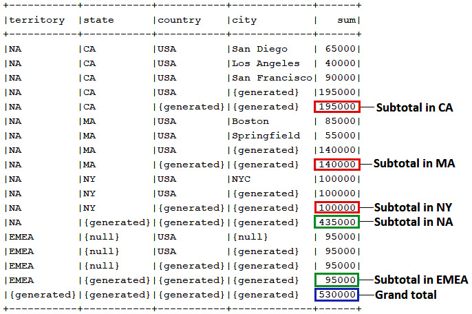
Figure 13.27 – ROLLUP output

As with ROLLUP, a CUBE group can also be perceived as a series of grouping sets. However, CUBE calculates all permutations of the cubed grouping expression along with the grand total. So, for n elements, CUBE produces 2n grouping sets. For instance GROUP BY CUBE (x, y, x) is equivalent to GROUP BY GROUPING SETS ((x, y, z), (x, y), (x, z), (y, z), (x), (y), (z), ()).

Let's apply CUBE for computing the sum of the internal budget for offices by state, country, and city. The query is shown here:

ctx.select(

 case_().when(grouping(OFFICE.STATE).eq(1), "{generated}")

  .else_(OFFICE.STATE).as("state"),

 case_().when(grouping(OFFICE.COUNTRY).eq(1), "{generated}")

  .else_(OFFICE.COUNTRY).as("country"),

 case_().when(grouping(OFFICE.CITY).eq(1), "{generated}")

  .else_(OFFICE.CITY).as("city"),

 sum(OFFICE.INTERNAL_BUDGET))

  .from(OFFICE)

  .where(OFFICE.COUNTRY.eq("USA"))

  .groupBy(cube(OFFICE.STATE, OFFICE.COUNTRY, OFFICE.CITY))

  .fetch();

Finally, let's talk about the GROUPING_ID() function. This function computes the decimal equivalent of the binary value obtained by concatenating the values returned by the GROUPING() functions applied to all the columns of the GROUP BY clause. Here is an example of using GROUPING_ID() via jOOQ groupingId():

ctx.select(

 case_().when(grouping(OFFICE.TERRITORY).eq(1), "{generated}")

  .else_(OFFICE.TERRITORY).as("territory"),

 ...

 case_().when(grouping(OFFICE.CITY).eq(1), "{generated}")

  .else_(OFFICE.CITY).as("city"),

 groupingId(OFFICE.TERRITORY, OFFICE.STATE, OFFICE.COUNTRY, 

            OFFICE.CITY).as("grouping_id"),

 sum(OFFICE.INTERNAL_BUDGET))

   .from(OFFICE)

   .where(OFFICE.COUNTRY.eq("USA"))

   .groupBy(rollup(OFFICE.TERRITORY, OFFICE.STATE, 

                   OFFICE.COUNTRY, OFFICE.CITY))

   .fetch();

The following screenshot shows a sample output:

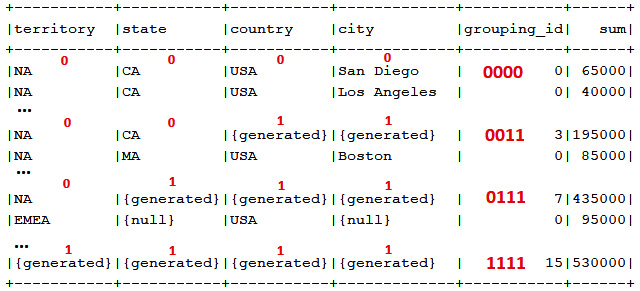
Figure 13.28 – GROUPING_ID() output

GROUPING_ID() can also be used in HAVING for creating conditions, as follows:

… .having(groupingId(OFFICE.TERRITORY, 

    OFFICE.STATE, OFFICE.COUNTRY, OFFICE.CITY).eq(3))…

The complete query is available in the GroupingRollupCube bundled code.

Summary

Working with SQL functions is such fun! They truly boost the SQL world and allow us to solve so many problems during data manipulation. As you saw in this chapter, jOOQ provides comprehensive support to SQL functions, covering regular and aggregate functions to the mighty window functions, ordered set aggregate functions (WITHIN GROUP), and so on. While we're on this topic, allow me to recommend the following article as a great read: https://blog.jooq.org/how-to-find-the-closest-subset-sum-with-sql/. In the next chapter, we tackle virtual tables (vtables).