For this exercise, we'll have a look at the raster module. We'll work with raster data in the form of Landsat 8 satellite images and look at ways to describe the data and use geoprocessing functionality from ArcGIS Online. As always, we'll start with importing the arcgis package and gis module, this time using an anonymous login:

In: import arcgis
    from arcgis.gis import GIS
    from IPython.display import display
    gis = GIS()

Next, we'll search for content—we'll specify that we're looking for imagery layers, the data type for imagery used for the raster module. We limit the results to a maximum of 2:

In: items = gis.content.search("Landsat 8 Views", item_type="Imagery 
    Layer",
    max_items=2)

Next, we'll display the items as follows:

In: for item in items:
        display(item)

The output shows the following two items:

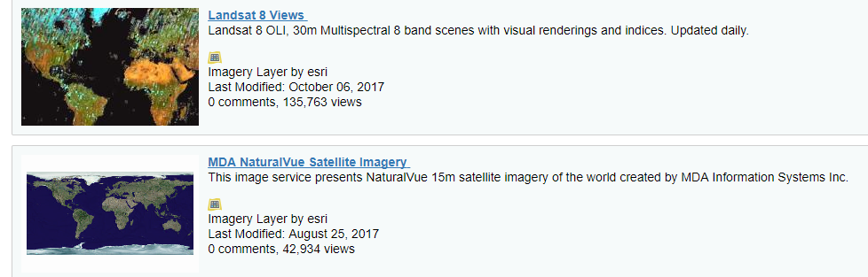
We're interested in the first item of the results. We can reference it as follows:

In: l8_view = items[0]

Let's now investigate this item a little more by clicking the blue Landsat 8 Views URL. It takes you to a web page with a description of the dataset. Have a look at the band numbers and their description. The API offers raster functions available on this landsat layer, which we'll get to in a minute. First, we'll access the imagery layer through the layers property of the item:

In: l8_view.layers

Next, we can reference and visualize the layer as follows:

In: l8_lyr = l8_view.layers[0]
    l8_lyr

The output shows the layer, covering the whole earth:

Having the image layer available as a Python object we can print all of available properties, returned, as before, in JSON:

In: l8_lyr.properties

A more visually attractive imagery layer item description can be printed using the following code:

In: from IPython.display import HTML
In: HTML(l8_lyr.properties.description)

Using a pandas dataframe, we can explore the different wavelength bands in more detail:

In:   import pandas as pd
In:   pd.DataFrame(l8_lyr.key_properties()['BandProperties'])

The output is now presented in a pandas dataframe object:

Now we'll get to the raster functions part. The API provides a set of raster functions to be used on the imagery layer that are rendered server-side and returned to the user. To minimize the output, the user needs to specify a location or area, whose screen extent will be used as input for a raster function. Raster functions can also be chained together and work on large datasets too. The following for loop displays all of the available raster functions available for this particular dataset:

In: for fn in l8_lyr.properties.rasterFunctionInfos: 
        print(fn['name'])

The output shows all of the available raster functions on a separate line:

This information is also present in the full properties list we printed out earlier. Next, we'll try out some of these raster functions on a map showing the area of Madrid, Spain. We'll start by creating an instance of the map:

In: map = gis.map('Madrid, Spain')

Then, we'll add our satellite image to the map widget, which we can use for various raster functions:

In: map.add_layer(l8_lyr)
    map

The output will look like this:

We'll now need to import the apply function from the raster module in order to apply the raster functions:

In: from arcgis.raster.functions import apply

First, we'll create a natural color image with dynamic range adjustment, using bands 4, 3, and 2:

In: natural_color = apply(l8_lyr, 'Natural Color with DRA')

Update the map as follows and see how it is different than before:

In: map.add_layer(natural_color)

The output will look like this:

We'll repeat the procedure, but this time we'll visualize the agricultural map:

In: agric = apply(l8_lyr, 'Agriculture')
In: map.add_layer(agric)

This raster function uses the bands 6, 5 and 2, referring to shortwave IR-1, near-IR and blue, respectively.  We can see that our study area shows all of the three following categories—vigorous vegetation is bright green, stressed vegetation dull green, and bare areas as brown. We can verify the results in our map widget:

As you can see, the raster module enables quick geoprocessing of raster imagery in the cloud, and returns and displays the results on your screen quickly. This is just one of the many raster functions of the module, and there is much more to discover. This concludes this exercise where we looked at how we search for raster imagery, display it, and use geoprocessing capabilities of ArcGIS Online using the ArcGIS API for Python’s raster module.