The inference of the probability of a long sequence, say w ₁ , ..., w _m, is typically infeasible. Calculating the joint probability of P(w ₁ , ... , w _m ) would be done by applying the following chain rule:

Especially the probability of the later words given the earlier words would be difficult to estimate from the data. This is why this joint probability is typically approximated by an independence assumption that the i^th word is only dependent on the n-1 previous words. We only model the joint probabilities of n sequential words called n-grams. Note that n-grams can be used to refer to other sequences of length n, such as n characters.

The inference of the joint distribution is approximated via n-gram models that split up the joint distribution in multiple independent parts. Note that n-grams are combinations of multiple sequential words, where n is the number of sequential words. For example, in the phrase the quick brown fox, we have the following n-grams:

Now if we have a huge corpus of text, we can find all the n-grams up until a certain n (typically 2 to 4) and count the occurrence of each n-gram in that corpus. From these counts, we can estimate the probabilities of the last word of each n-gram, given the previous n-1 words:

The independence assumption that the i^th word is only dependent on the previous n-1 words can now be used to approximate the joint distribution.

For example, for a unigram, we can approximate the joint distribution by:

For a trigram, we can approximate the joint distribution by:

We can see that based on the vocabulary size, the number of n-grams grows exponentially with n. For example, if a small vocabulary contains 100 words, then the number of possible 5-grams would be 100⁵ = 10,000,000,000 different 5-grams. In comparison, the entire works of Shakespeare contain around 30,000 different words, illustrating the infeasibility of using n-grams with a large n. Not only is there the issue of storing all the probabilities, we would also need a very large text corpus to create decent n-gram probability estimations for larger values of n. This problem is what is known as the curse of dimensionality. When the number of possible input variables (words) increases, the number of different combinations of these input values increases exponentially. This curse of dimensionality arises when the learning algorithm needs at least one example per relevant combination of values, which is the case in n-gram modeling. The larger our n, the better we can approximate the original distribution and the more data we would need to make good estimations of the n-gram probabilities.

In the previous section, we illustrated the curse of dimensionality when modeling text with n-grams. The number of n-grams we need to count grows exponentially with n and with the number of words in the vocabulary. One way to overcome this curse is by learning a lower dimensional, distributed representation of the words [20]. This distributed representation is created by learning an embedding function that transforms the space of words into a lower dimensional space of word embeddings, as follows:

V-words from the vocabulary are transformed into one-hot encoding vectors of size V (each word is encoded uniquely). The embedding function then transforms this V-dimensional space into a distributed representation of size D (here D=4).

The idea is that the learned embedding function learns semantic information about the words. It associates each word in the vocabulary with a continuous-valued vector representation, the word embedding. Each word corresponds to a point in this embedding space where different dimensions correspond to the grammatical or semantic properties of these words. The goal is to ensure that the words close to each other in this embedding space should have similar meanings. This way, the information that some words are semantically similar can be exploited by the language model. For example, it might learn that "fox" and "cat" are semantically related and that both "the quick brown fox" and "the quick brown cat" are valid phrases. A sequence of words can then be transformed into a sequence of embedding vectors that capture the characteristics of these words.

It is possible to model the language model via a neural network and learn this embedding function implicitly. We can learn a neural network that given a sequence of n-1 words (w_t-n+1 , …, w_t-1) tries to output the probability distribution of the next word, that is, w_t. The network is made up of different parts.

The embedding layer takes the one-hot representation of the word w _i and converts it into its embedding by multiplying it with the embedding matrix C. This computation can be efficiently implemented by a table lookup. The embedding matrix C is shared over all the words, so all words use the same embedding function. C is represented by a V * D matrix, where V is the size of the vocabulary and D the size of the embedding. The resulting embeddings are concatenated into a hidden layer; after this, a bias b and a nonlinear function, such as tanh, can be applied. The output of the hidden layer is thus represented by the function z = tanh(concat(w _t-n+1 , …, w _t-1 ) + b). From the hidden layer, we can now output the probability distribution of the next word w _t by multiplying the hidden layer with U. This maps the hidden layer to the word space, adding a bias b and applying the softmax function to get a probability distribution. The final layer computes softmax(z*U +b). This network is illustrated in the following figure:

A neural network language model that outputs the probability distribution of the word w_t, given the words w_t-1 ... w_t-n+1. C is the embedding matrix.

This model simultaneously learns an embedding of all the words in the vocabulary and a model of the probability function for sequences of words. It is able to generalize this probability function to sequences of words not seen during training, thanks to these distributed representations. A specific combination of words in the test set might not be seen in the training set, but a sequence with similar embedding features is much more likely to be seen during training.

A 2D projection of some word embeddings is illustrated in the following figure. It can be seen that words that are semantically close are also close to each other in the embedding space.

Related words in a 2D embedding space are close to each other in this space [21]

Word embeddings can be trained unsupervised on a large corpus of text data. This way, they are able to capture general semantic information between words. The resulting embeddings can now be used to improve the performance of other tasks where there might not be a lot of labeled data available. For example, a classifier trying to classify the sentiment of an article might be trained on using previously learned word embeddings, instead of one-hot encoding vectors. This way, the semantic information of the words becomes readily available for the sentiment classifier. Because of this, a lot of research has gone into creating better word embeddings without focusing on learning a probability function over sequences of words. For example, a popular word embedding model is word2vec [22], [23].

A surprising result is that these word embeddings can capture analogies between words as differences. It might, for example, capture that the difference between the embedding of "woman" and "man" encodes the gender and that this difference is the same in other gender-related words such as "queen" and "king."

Word embeddings can capture semantic differences between words [24]

embed(woman) - embed(man) ? embed(aunt) - embed(uncle)

embed(woman) - embed(man) ? embed(queen) - embed(king)

While the previous feedforward network language model can overcome the curse of dimensionality of modeling a large vocabulary input, it is still limited to only modeling fixed length word sequences. To overcome this issue, we can use RNNs to build an RNN language model that is not limited by fixed length word sequences [25]. These RNN-based models can then not only cluster similar words in the input embedding, but can also cluster similar histories in the recurrent state vector.

One issue with these word-based models is computing the output probabilities, P(w _i | context), of each word in the vocabulary. We get these output probabilities by using a softmax over all word activations. For a small vocabulary V of 50,000 words, this would need a |S| * |V| output matrix, where |V| is the size of the vocabulary and |S| the size of the state vector. This matrix is huge and would grow even more when we increase our vocabulary. And because softmax normalizes the activation of a single word by a combination of all other activations, we need to compute each activation to get the probability of a single word. Both illustrate the difficulty of computing the softmax over a large vocabulary; a lot of parameters are needed to model the linear transformation before the softmax, and the softmax itself is computationally intensive.

There are ways to overcome this issue, for example, by modeling the softmax function as a binary tree, essentially only needing log(|V|) computations the calculate to final output probability of a single word [26].

Instead of going into these workarounds in detail, let's check out another variant of language modeling that is not affected by these large vocabulary issues.

To train a good language model, we need a lot of data. For our example, we will learn about a model based on the English translation of Leo Tolstoy's "War and peace." This book contains more than 500,000 words, making it the perfect candidate for our small example. Since it's in the public domain, "War and peace" can be downloaded as plain text for free from Project Gutenberg. As part of preprocessing, we will remove the Gutenberg license, book information, and table of contents. Next, we will strip out newlines in the middle of sentences and reduce the maximum number of consecutive newlines allowed to two.

To feed the data into the network, we will have to convert it into a numerical format. Each character will be associated with an integer. In our example, we will extract a total of 98 different characters from the text corpus. Next, we will extract input and targets. For each input character, we will predict the next character. Because we are training with truncated BPTT, we will make all the batches follow up on each other to exploit the continuity of the sequence. The process of converting the text into a list of indices and splitting it up in to batches of input and targets is illustrated in the following figure:

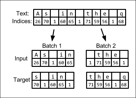
Converting text into input and target batches of integer labels with length 5. Note that batches follow on to each other.

The network we will train will be a two-layer LSTM network with 512 cells in each layer. We will train this network with truncated BPTT, so we will need to store the state between batches.

First, we need to define placeholders for our input and targets. The first dimension of both the input and targets is the batch size, the number of examples processed in parallel. The second dimension will be the dimension along the text sequence. Both these placeholders take batches of sequences where the characters are represented by their index:

inputs = tf.placeholder(tf.int32, (batch_size, sequence_length))
targets = tf.placeholder(tf.int32, (batch_size, sequence_length))

To feed the characters to the network, we need to transform them into a vector. We will transform them into one-hot encoding, which means that each character is going to be transformed into a vector with length equal to the size of the number of different characters in the dataset. This vector will be all zeros, except the cell that corresponds to its index, which will be set to 1. This can be done easily in TensorFlow with the following line of code:

one_hot_inputs = tf.one_hot(inputs, depth=number_of_characters)

Next, we will define our multilayer LSTM architecture. First we need to define the LSTM cells for each layer (lstm_sizes is a list of sizes for each layer, for example (512, 512), in our case):

cell_list = (tf.nn.rnn_cell.LSTMCell(lstm_size) for lstm_size in lstm_sizes)

Then, we wrap these cells in a single multilayer RNN cell using this:

multi_cell_lstm = tf.nn.rnn_cell.MultiRNNCell(cell_list)

To store the state between the batches, we need to get the initial state of the network and wrap it in the variable to be stored. Note that for computational reasons, TensorFlow stores LSTM states in a tuple of two separate tensors (c and h from the Long Short Term Memory section ). We can flatten this nested data structure with the flatten method, wrap each tensor in a variable, and repack it as the original structure with the pack_sequence_as method:

initial_state = self.multi_cell_lstm.zero_state(batch_size, tf.float32)
# Convert to variables so that the state can be stored between batches
state_variables = tf.python.util.nest.pack_sequence_as(
    self.initial_state,
    (tf.Variable(var, trainable=False) 
     for var in tf.python.util.nest.flatten(initial_state)))

Now that we have the initial state defined as a variable, we can start unrolling the network through time. TensorFlow provides the dynamic_rnn method that does this unrolling dynamically as per the sequence length of the input. This method will return a tuple consisting of a tensor representing the LSTM output and the final state:

lstm_output, final_state = tf.nn.dynamic_rnn(
    cell=multi_cell_lstm, inputs=one_hot_inputs,    
    initial_state=state_variable)

Next, we need to store the final state as the initial state for the next batch. We use the variable assign method to store each final state in the right initial state variable. The control_dependencies method is used to force that the state update to run before we return the LSTM output:

store_states = (
    state_variable.assign(new_state)
    for (state_variable, new_state) in zip(
        tf.python.util.nest.flatten(self.state_variables),
        tf.python.util.nest.flatten(final_state)))
with tf.control_dependencies(store_states):
    lstm_output = tf.identity(lstm_output)

To get the logit output from the final LSTM output, we need to apply a linear transformation to the output so it can have batch size * sequence length * number of symbols as its dimensions. Before we apply this linear transformation, we need to flatten the output to a matrix of the size number of outputs * number of output features:

output_flat = tf.reshape(lstm_output, (-1, lstm_sizes(-1)))

We can then define and apply the linear transformation with a weight matrix W and bias b to get the logits, apply the softmax function, and reshape it to a tensor of the size batch size * sequence length * number of characters:

# Define output layer
logit_weights = tf.Variable(
    tf.truncated_normal((lstm_sizes(-1), number_of_characters), stddev=0.01))
logit_bias = tf.Variable(tf.zeros((number_of_characters)))
# Apply last layer transformation
logits_flat = tf.matmul(output_flat, self.logit_weights) + self.logit_bias
probabilities_flat = tf.nn.softmax(logits_flat)
# Reshape to original batch and sequence length
probabilities = tf.reshape(
    probabilities_flat, (batch_size, -1, number_of_characters))

LSTM character language model unfolded

Now that we have defined the input, targets, and architecture of our network, let's define how to train it. The first step in training is defining a loss function that we want to minimize. This loss function describes the cost of outputting a wrong sequence of characters, given the input and targets. Because we are predicting the next character considering the previous characters, it is a classification problem and we will use cross-entropy loss. We do this by using the sparse_softmax_cross_ entropy_with_logits TensorFlow function. This function takes the logit output of the network as input (before the softmax) and targets as class labels and computes the cross-entropy loss of each output with respect to its target. To reduce the loss over the full sequence and all the batches, we take the mean value of all of them.

Note that we flatten the targets to a one-dimensional vector first to make them compatible with the flattened logit output from our network:

# Flatten the targets to be compatible with the flattened logits
targets_flat = tf.reshape(targets, (-1, ))
# Get the loss over all outputs
loss = tf.nn.sparse_softmax_cross_entropy_with_logits(
     logits_flat, targets_flat)
# Reduce the loss to single value over all outputs
loss = tf.reduce_mean(loss)

Now that we have this loss function defined, it is possible to define the training operation in TensorFlow that will optimize our network of input and target batches. To execute the optimization, we will use the Adam optimizer; this helps stabilize gradient updates. The Adam optimizer is just a specific way of performing gradient descent in a more controlled way [28]. We will also clip the gradients to prevent exploding gradients:

# Get all variables that need to be optimised
trainable_variables = tf.trainable_variables()
# Compute and clip the gradients
gradients = tf.gradients(loss, trainable_variables)
gradients, _ = tf.clip_by_global_norm(gradients, 5)
# Apply the gradients to those variables with the Adam optimisation algorithm.
optimizer = tf.train.AdamOptimizer(learning_rate=2e-3)
train_op = optimizer.apply_gradients(zip(gradients, trainable_variables))

Having defined all the TensorFlow operations required for training, we can now start with the optimization in mini batches. If data_feeder is a generator that returns consecutive batches of input and targets, then we can train these batches by iteratively feeding in the input and target batches. We reset the initial state every 100 mini batches so that the network learns how to deal with the initial states in the beginning of sequences. You can save the model with a TensorFlow saver to reload it for sampling later:

with tf.Session() as session:
    session.run(tf.initialize_all_variables())
    for i in range(minibatch_iterations):
        input_batch, target_batch = next(data_feeder)
        loss, _ = sess.run(
            (loss, train_op),
            feed_dict={ inputs: input_batch,targets: target_batch})
    # Reset initial state every 100 minibatches
        if i % 100 == 0 and i != 0:
            for state in tf.python.util.nest.flatten(
                    state_variables):
                session.run(state.initializer)

Once our model is trained, we might want to sample the sequences from this model to generate text. We can initialize our sampling architecture with the same code we used for training the model, but we'd need to set batch_size to 1 and sequence_length to None. This way, we can generate a single string and sample sequences of different lengths. We can then initialize the parameters of the model with the parameters saved after training. To start with the sampling, we feed in an initial string (prime_string) to prime the state of the network. After this string is fed in, we can sample the next character based on the output distribution of the softmax function. We can then feed in this sampled character and get the output distribution for the next one. This process can be continued for a number of steps until a string of a specified size is generated:

# Initialize state with priming string
for character in prime_string:
    character_idx = label_map(character)
    # Get output distribution of next character
    output_distribution = session.run(
        probabilities, 
        feed_dict={inputs: np.asarray(((character_idx)))})
# Start sampling for sample_length steps
for _ in range(sample_length):
    # Sample next character according to output distribution
    sample_label = np.random.choice(
        labels, size=(1), p=output_distribution(0, 0))
    output_sample += sample_label
    # Get output distribution of next character
    output_distribution = session.run(
       probabilities,
       feed_dict={inputs: np.asarray((label_map(character))))

Now that we have our code for training and sampling, we can train the network on Leo Tolstoy's War and Peace and sample what the network has learned every couple of batch iterations. Let's prime the network with the phrase "She was born in the year" and see how it completes it during training.

After 500 batches, we get this result: She was born in the year sive but us eret tuke Toffhin e feale shoud pille saky doctonas laft the comssing hinder to gam the droved at ay vime. The network has already picked up some distribution of characters and has come up with things that look like words.

After 5,000 batches, the network picks up a lot of different words and names: "She was born in the year he had meaningly many of Seffer Zsites. Now in his crownchy-destruction, eccention, was formed a wolf of Veakov one also because he was congrary, that he suddenly had first did not reply." It still invents plausible looking words likes "congrary" and "eccention".

After 50,000 batches, the network outputs the following text: She was born in the year 1813. At last the sky may behave the Moscow house there was a splendid chance that had to be passed the Rostóvs', all the times: sat retiring, showed them to confure the sovereigns." The network seems to have figured out that a year number is a very plausible words to follow up our prime string. Short strings of words seem to make sense, but the sentences on their own don't make sense yet.

After 500,000 batches, we stop the training and the network outputs this: "She was born in the year 1806, when he entered his thought on the words of his name. The commune would not sacrifice him : "What is this?" asked Natásha. "Do you remember?"". We can see that the network is now trying to make sentences, but the sentences are not coherent with each other. What is remarkable is that it models small conversations in full sentences at the end, including quotes and punctuation.

While not perfect, it is remarkable how the RNN language model is able to generate coherent phrases of text. We would like to encourage you at this point to experiment with different architectures, increase the size of the LSTM layers, put a third LSTM layer in the network, download more text data from the Internet, and see how much you can improve the current model.

The language models we have discussed so far are used in many different applications, ranging from speech recognition to creating intelligent chat bots that are able to build a conversation with a user. In the next section, we will briefly discuss deep learning speech recognition models in which language models play an important part.