
The neural network architectures we discussed in the previous chapters take in fixed sized input and provide fixed sized output. Even the convolutional networks used in image recognition (Chapter 5, Image Recognition) are flattened into a fixed output vector. This chapter will lift us from this constraint by introducing Recurrent Neural Networks (RNNs). RNNs help us deal with sequences of variable length by defining a recurrence relation over these sequences, hence the name.
The ability to process arbitrary sequences of input makes RNNs applicable for tasks such as language modeling (see section on Language Modelling) or speech recognition (see section on Speech Recognition). In fact, in theory, RNNs can be applied to any problem since it has been proven that they are Turing-Complete [1]. This means that theoretically, they can simulate any program that a regular computer would not be able to compute. As an example of this, Google DeepMind has proposed a model named "Neural Turing Machines", which can learn how to execute simple algorithms, such as sorting [2].
In this chapter, we will cover the following topics:
- How to build and train a simple RNN, based on a toy problem
- The problem of vanishing and exploding gradients in RNN training and how to solve them
- The LSTM model for long-term memory learning
- Language modeling and how RNNs can be applied to this problem
- A brief introduction to applying deep learning to speech recognition
RNNs get their name because they recurrently apply the same function over a sequence. An RNN can be written as a recurrence relation defined by this function:
Here St —the state at step t—is computed by the function f from the state in the previous step, that is t-1, and an input Xt at the current step. This recurrence relation defines how the state evolves step by step over the sequence via a feedback loop over previous states, as illustrated in the following figure:
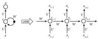
Figure from [3]
Left: Visual illustration of the RNN recurrence relation: S t = S t-1 * W + X t * U. The final output will be o t = V*S t
Right: RNN states recurrently unfolded over the sequence t- 1, t, t+1. Note that the parameters U, V, and W are shared between all the steps.
Here f can be any differentiable function. For example, a basic RNN is defined by the following recurrence relation:
Here W defines a linear transformation from state to state, and U is a linear transformation from input to state. The tanh function can be replaced by other transformations, such as logit, tanh, or ReLU. This relation is illustrated in the following figure where Ot is the output generated by the network.
For example, in word-level language modeling, the input X will be a sequence of words encoded in input vectors (X 1 … X t …). The state S will be a sequence of state vectors (S 1 … S t … ). And the output O will be a sequence of probability vectors (O 1 … O t … ) of the next words in the sequence.
Notice that in an RNN, each state is dependent on all previous computations via this recurrence relation. An important implication of this is that RNNs have memory over time because the states S contain information based on the previous steps. In theory, RNNs can remember information for an arbitrarily long period of time, but in practice, they are limited to look back only a few steps. We will address this issue in more detail in section on Vanishing and exploding gradients.
Because RNNs are not limited to processing input of fixed size, they really expand the possibilities of what we can compute with neural networks, such as sequences of different lengths or images of varied sizes. The next figure visually illustrates some combinations of sequences we can make. Here's a brief note on these combinations:
- One-to-one: This is non-sequential processing, such as feedforward neural networks and convolutional neural networks. Note that there isn't much difference between a feedforward network and applying an RNN to a single time step. An example of one-to-one processing is the image classification from chapter (See Chapter 5, Image Recognition).
- One-to-many: This generates a sequence based on a single input, for example, caption generation from an image [4].
- Many-to-one: This outputs a single result based on a sequence, for example, sentiment classification from text.
- Many-to-many indirect: A sequence is encoded into a state vector, after which this state vector is decoded into a new sequence, for example, language translation [5], [6].
- Many-to-many direct: This outputs a result for each input step, for example, frame phoneme labeling in speech recognition (see the Speech recognition section).

Image from [7]
RNNs expand the possibilities of what we can compute with neural networks—Red: input X, Green: states S, Blue: outputs O.
In the previous section, we briefly discussed what RNNs are and what problems they can solve. Let's dive into the details of an RNN and how to train it with the help of a very simple toy example: counting ones in a sequence.
In this problem, we will teach the most basic RNN how to count the number of ones in the input and output the result at the end of the sequence. We will show an implementation of this network in Python and NumPy. An example of input and output is as follows:
In:  (0, 0, 0, 0, 1, 0, 1, 0, 1, 0)
Out:  3
The network we are going to train is a very basic one and is illustrated in the following figure:

Basic RNN for counting ones in the input
The network will have only two parameters: an input weight U and a recurrence weight W. The output weight V is set to 1 so we just read out the last state as the output y. The recurrence relation defined by this network is S t = S t-1 * W + X t * U. Note that this is a linear model since we don't apply a nonlinear function in this formula. This function can be defined in terms of code as follows:
def step(s, x, U, W):
    return x * U + s * W
Because 3 is the number we want to output and there are three ones, a good solution to this is to just get the sum of the input across the sequence. If we set U=1, then whenever an input is received, we will get its full value. If we set W=1, then the value we would accumulate will never decay. So for this example, we would get the desired output: 3.
Nevertheless, the training and implementation of this neural network will be interesting, as we will see in the rest of this section. So let's see how we could get this result through backpropagation.
The backpropagation through time algorithm is the typical algorithm we use to train recurrent networks [8]. The name already implies that it is based on the backpropagation algorithm we discussed in Chapter 2, Neural Networks.
If you understand regular back-propagation, then backpropagation through time is not too difficult to understand. The main difference is that the recurrent network needs to be unfolded through time for a certain number of time steps. This unfolding is illustrated in the preceding figure (Basic RNN for counting ones in the input). Once the unfolding is complete, we end up with a model that is quite similar to a regular multilayer feedforward network. The only differences are that each layer has multiple input (the previous state, which is S t-1), and the current input (X t) and the parameters (here U and W) are shared between each layer.
The forward pass unwraps the RNN along the sequence and builds up a stack of activities for each step. The forward step with a batch of input sequences X can be implemented as follows:
def forward(X, U, W):
    # Initialize the state activation for each sample along the sequence
    S = np.zeros((number_of_samples, sequence_length+1))
    # Update the states over the sequence
    for t in range(0, sequence_length):
        S[:,t+1] = step(S[:,t], X[:,t], U, W)  # step function
    return S
After this forward step, we have the resulting activations, represented by S, for each step and each sample in the batch. Because we want to output more or less continuous output (sum of all ones), we use the mean squared error cost function to define our output cost with respect to the targets and output y, as follows:
cost = np.sum((targets – y)**2)
Now that we have our forward step and cost function, we can define how the gradient is propagated backward. First, we need to get the gradient of the output y with respect to the cost function (??/?y).
Once we have this gradient, we can propagate it backward through the stack of activities we built during the forward step. This backward pass pops activities off the stack to accumulate the error derivatives at each time step. The recurrence relation to propagate this gradient through the network can be written as follows:

The gradients of the parameters are accumulated with this:


In the following implementation, the gradients for U and W are accumulated during gU and gW, respectively, during the backward step:
def backward(X, S, targets, W):
    # Compute gradient of output
    y = S[:,-1]  # Output `y` is last activation of sequence
    # Gradient w.r.t. cost function at final state
    gS = 2.0 * (y - targets)
    # Accumulate gradients backwards
    gU, gW = 0, 0  # Set the gradient accumulations to 0
    for k in range(sequence_len, 0, -1):
        # Compute the parameter gradients and accumulate the results.
        gU += np.sum(gS * X[:,k-1])
        gW += np.sum(gS * S[:,k-1])
        # Compute the gradient at the output of the previous layer
        gS = gS * W
    return gU, gW
We can now try to use gradient descent to optimize our network:
learning_rate = 0.0005
# Set initial parameters
parameters = (-2, 0)  # (U, W)
# Perform iterative gradient descent
for i in range(number_iterations):
    # Perform forward and backward pass to get the gradients
    S = forward(X, parameters(0), parameters(1))
    gradients = backward(X, S, targets, parameters(1))
    # Update each parameter `p` by p = p - (gradient * learning_rate).
    # `gp` is the gradient of parameter `p`
    parameters = ((p - gp * learning_rate)
                  for p, gp in zip(parameters, gradients))
There is an issue though. Notice that if you try to run this code, the final parameters U and W tend to end up as Not a Number (NaN). Let's try to investigate what happened by plotting the parameter updates over an error surface, as shown in the following figure. Notice that the parameters slowly move toward the optimum (U=W=1) until it overshoots and hits approximately (U=W=1.5). At this point, the gradient values just blow up and make the parameter values jump outside the plot. This problem is known as exploding gradients. The next section will explain why this happens in detail and how to prevent it.

Parameter updates plotted on an error surface via a gradient descent. The error surface is plotted on a logarithmic color scale
RNNs can be harder to train than feedforward or convolutional networks. Some difficulties arise due to the recurrent nature of the RNN where the same weight matrix is used to compute all the state updates [9], [10].
The end of the last section, the preceding figure, illustrated the exploding gradient, which brings RNN training to an unstable state due to the blowing up of long-term components. Besides the exploding gradient problem, there is also the vanishing gradient problem where the opposite happens. Long-term components go to zero exponentially fast, and the model is unable to learn from temporally distant events. In this section, we will explain both the problems in detail and also how to deal with them.
Both exploding and vanishing gradients arise from the fact that the recurrence relation that propagates the gradient backward through time forms a geometric sequence:

In our simple linear RNN, the gradient grows exponentially if |W| > 1. This is known as the exploding gradient (for example, 50 time steps over W=1.5 is W50 = 1.550 ˜≈6 * 108 ). The gradient shrinks exponentially if |W| < 1; this is known as the vanishing gradient (for example, 20 time steps over W=0.6 is W20 = 0.620 ˜≈3*10-5 ). If the weight parameter W is a matrix instead of a scalar, this exploding or vanishing gradient is related to the largest eigenvalue (ρ) of W (also known as a spectral radius). It is sufficient for ρ < 1 for the gradients to vanish, and it is necessary for ρ > 1 for them to explode.
The following figure visually illustrates the concept of exploding gradients. What happens is that the cost surface we are training on is highly unstable. Using small steps, we might move to a stable part of the cost function, where the gradient is low, and suddenly hit upon a jump in cost and a corresponding huge gradient. Because this gradient is so huge, it will have a big effect on our parameters. They will end up in a place on the cost surface that is far from where they originally were. This makes gradient descent learning unstable and even impossible in some cases.

Illustration of an exploding gradient [11]
We can counter the effects of exploding gradients by controlling the size our gradients can grow to. Some examples of solutions are:
- Gradient clipping, where we threshold the maximum value a gradient can get [11].
- Second order optimization (Newton's method), where we model the curvature of the cost function. Modeling the curvature allows us to take big steps in low-curvature scenarios and small steps in high-curvature scenarios. For computational reasons, typically only an approximation of the second order gradient is used [12].
- Optimization methods, such as momentum [13] or RmsProp that rely less on the local gradient [14].
For example, we can retrain our network that wasn't able to converge (refer the preceding figure of Illustration of an exploding gradient) with the help of Rprop [15]. Rprop is a momentum-like method that only uses the sign of the gradient to update the momentum parameters, and it is thus not affected by exploding gradients. If we run Rprop optimization, we can see that the training converges in the following figure. Notice that while the training starts in a high gradient region (U=-1.5, W=2), it converges fast until it finds the optimum at (U =W=1).

Parameter updates via Rprop plotted on an error surface. Error surface is plotted on a logarithmic scale.
The vanishing gradient problem is the inverse of the exploding gradient problem. The gradient decays exponentially over the number of steps. This means that the gradients in earlier states become extremely small, and the ability to retain the history of these states vanishes. The small gradients from earlier time steps are outcompeted by the larger gradients from more recent time steps. Hochreiter and Schmidhuber [16] describe this as follows: Backpropagation through time is too sensitive to recent distractions.
This problem is more difficult to detect because the network will still learn and output something (unlike in the exploding gradients case). It just won't be able to learn long-term dependencies. People have tried to tackle this problem with solutions similar to the ones we have for exploding gradients, such as second order optimization or momentum. These solutions are far from perfect, and learning long-term dependencies with simple RNNs is still very difficult. Thankfully, there is a clever solution to the vanishing gradient problem that uses a special architecture made up of memory cells. We will discuss this architecture in detail in the next section.
In theory, simple RNNs are capable of learning long-term dependencies, but in practice, due to the vanishing gradient problem, they only seem to limit themselves to learning short-term dependencies. Hochreiter and Schmidhuber studied this problem extensively and came up with a solution called Long Short Term Memory (LSTM) [16]. LSTMs can handle long-term dependencies due to a specially crafted memory cell. They work so well that most of the current accomplishments in training RNNs on a variety of problems are due to the use of LSTMs. In this section, we will explore how this memory cell works and how it solves the vanishing gradient issue.
The key idea of LSTM is the cell state, of which the information can only be explicitly written in or removed so that the cell state stays constant if there is no outside interference. This cell state for time t is illustrated as c t in the next figure.
The LSTM cell state can only be altered by specific gates, which are a way to let information pass through. These gates are composed of a logistic sigmoid function and element-wise multiplication. Because the logistic function only outputs values between 0 and 1, the multiplication can only reduce the value running through the gate. A typical LSTM is composed of three gates: a forget gate, input gate, and output gate. These are all illustrated as f, i, and o, in the following figure. Note that the cell state, input, and output are all vectors, so the LSTM can hold a combination of different information blocks at each time step. Next, we will describe the workings of each gate in more detail.


LSTM cell
xt, ct, ht are the input, cell state, and LSTM output at time t, respectively.
The first gate in LSTM is the forget gate; it is called so because it decides whether we want to erase the cell state or not. This gate was not in the original LSTM proposed by Hochreiter; it was proposed by Gers and others [17]. The forget gate bases its decision on the previous output h t-1 and current input xt . It combines this information and squashes them by a logistic function so that it outputs a number between 0 and 1 for each block of the cell's vector. Because of the element-wise multiplication with the cell, an output of 0 erases a specific cell block completely and an output of 1 leaves all of the information in that cell blocked. This means that the LSTM can get rid of irrelevant information in its cell state vector.
The next gate decides what new information is going to be added to the memory cell. This is done in two parts. The first part decides whether information is going to be added. As in the input gate, its bases it decision on ht-1 and xt and outputs 0 or 1 through the logistic function available for each cell block of the cell's vector. An output of 0 means that no information is added to that cell block's memory. As a result, the LSTM can store specific pieces of information in its cell state vector:
The input to be added, a t, is derived from the previous output (h t-1) and the current input (xt) and is transformed via a tanh function:
The forget and input gates completely decide the new cell by adding the old cell state with the new information to add:
The last gate decides what the output is going to be. The output gate takes h t-1 and xt as input and outputs 0 or 1 through the logistic function available for each cell block's memory. An output of 0 means that the cell block doesn't output any information, while an output of 1 means that the full cell block's memory is transferred to the output of the cell. The LSTM can thus output specific blocks of information from its cell state vector:
The final value outputted is the cell's memory transferred by a tanh function:
Because all these formulas are derivable, we can chain LSTM cells together just like we chain simple RNN states together and train the network via backpropagation through time.
Now how does the LSTM protect us from vanishing gradients? Notice that the cell state is copied identically from step to step if the forget gate is 1 and the input gate is 0. Only the forget gate can completely erase the cell's memory. As a result, memory can remain unchanged over a long period of time. Also, notice that the input is a tanh activation added to the current cell's memory; this means that the cell memory doesn't blow up and is quite stable.
How the LSTM is unrolled in practice is illustrated in the following figure.
Initially, the value of 4.2 is given to the network as input; the input gate is set to 1 so the complete value is stored. Then for the next two time steps, the forget gate is set to 1. So the entire information is kept throughout these steps and no new information is being added because the input gates are set to 0. Finally, the output gate is set to 1, and 4.2 is outputted and remains unchanged.

Unrolling LSTM through time [18]
While the LSTM network described in the preceding diagram is a typical LSTM version used in most applications, there are many variants of LSTM networks that combine different gates in different orders [19]. Getting into all these different architectures is out of the scope of this book.