This chapter explains the different image manipulation nodes and their utilization procedures that are available in Blender Compositor. These nodes play a major role in attaining the desired look. The following is a list of topics covered in this chapter:
- The Bright/Contrast node
- The Hue Saturation Value node
- The Color Correction node
- Significance of Gain, Gamma, and Lift
- Significance of Midtones, Highlights, and Shadows
- The RGB Curves node
- The Color Balance node
- The Mix node
- The Gamma node
- The Invert node
- The Hue Correct node
- Transformation nodes
Image manipulation is the main phase for establishing a predetermined look in compositing. This stage mostly involves grading, merging, transforming, and resizing of the footage to achieve the desired look of the film. Blender Compositor is equipped with various tool nodes to perform these tasks.
The brightness of an image signifies the amount of light that is reflecting or radiating from it. Increasing or decreasing the brightness of a node proportionally changes the light reflection intensities of the input image as shown in following screenshot:

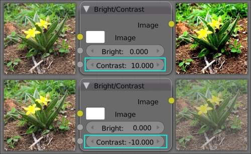
The contrast of an image signifies the luminance and/or color variation; in other words, the separation between the darkest and brightest areas of the image. Increasing the contrast emphasizes the distance between the dark and bright pixels in the image, thus making shadows darker and highlights brighter. This effect makes parts of the image pop up, making it a vibrant image. Decreasing the contrast makes the shadows lighter and highlights darker, making the image dull and less interesting. The following screenshot shows the effect of increasing and decreasing the contrast value on the Bright/Contrast node:
The Hue Saturation Value node provides a visual spectrum-based image control. The input image can be modified using the hue shift, which ranges from red to violet.
Using the Hue slider, the image hue can be shifted in the visible spectrum range. At the default value of 0.5, the hue doesn't affect the image. Reducing the value from 0.5 to 0 adds more cyan to the image, and increasing the value from 0.5 to 1 adds more reds and greens.
Saturation alters the strength of a hue tone in the image. A value of 0 removes the hue tones, making the image greyscale. A value of 2 doubles the strength of the hue tones.

The Color Correction node provides three dimensional controls on the input image as shown in following screenshot. As the first dimension, all vertical columns provide control on Saturation, Contrast, Gamma, Gain, and Lift. As the second dimension, all horizontal rows provide control on Master, Highlights, Midtones, and Shadows. The third dimensional control is Red, Green, and Blue. This node provides numerous combinations to arrive at a desired result through the use of these three dimensional controls.

The tonal information of the image can be divided into Shadows, Midtones, and Highlights. As shown in the following screenshot, this information can be represented as a histogram. In this representation, the left-hand values relate to the dark tones (Shadows), the middle values relate to Midtones, and the right-hand values relate to Highlights.
The Midtones Start and Midtones End sliders of the Color Correction node provide flexibility to alter the range between Shadows, Midtones, and Highlights using the luminance of the input image. These sliders don't consider the Red, Green, and Blue checkboxes. Controlling the tonal information through the Master attributes influences the complete range in the histogram curve of the image, thereby affecting the whole image.

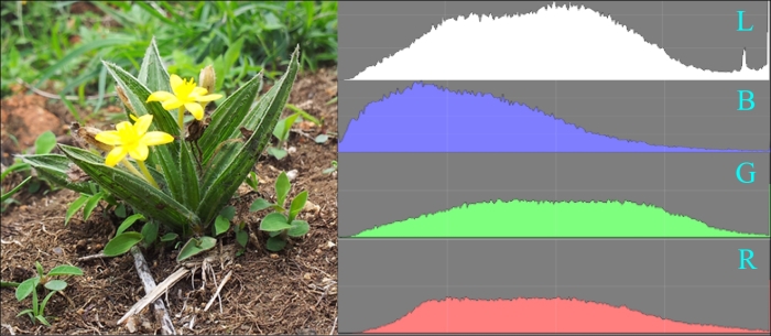
This level of control can be extended to individual red (R), green (G), blue (B), and luminance (L) channels of the image to gain more precision. The following screenshot displays histograms of the individual channels:
To arrive at a desired result quicker when using a Color Correction node, understanding the difference in control between Gamma, Gain, and Lift is vital. These terms can be understood better using an input (x axis) versus output (y axis) plot, as seen in following screenshot:

Each of these three properties controls the specific tonal information of an image, summarized as follows:
The RGB Curves node provides a Bezier-curve-based control for image grading. This curve represents an input (x axis) versus output (y axis) plot. Modifying this curve remaps the output range, thereby providing a grading effect. This node also provides controls to set up black and white levels for the input image.
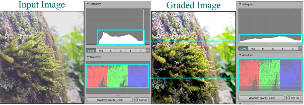
A flat image that has all pixel values in the midtones range can be graded to redistribute the pixel values to occupy the complete range of shadows, midtones, and highlights. This makes the image more vibrant and interesting. An example of this grading is shown in the following screenshot. The waveforms and histograms of both the images show the redistribution of pixel values to occupy the complete range and provide a better graded image.
Grading with this node can be done using Bezier curve or by tweaking the black and white levels. An appropriate technique can be adapted based on the task.
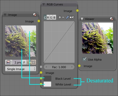
The variation between the black and white levels of an image signifies its contrast. Using the RGB Curves node to increase an image's contrast, instead of using a Bright/Contrast node, gives the advantage of picking samples from the input image, The darkest and the brightest levels of the input image can be picked as black and white levels respectively, as shown in following screenshot. You can pick a sample using the selector that pops up below the color wheel when either Black Level or White Level is clicked on.

This method not only alters the contrast but also changes hue tones. This change can be nullified by desaturating the black and white levels to zero using the saturation (S) slider in the HSV mode. The following screenshot shows a change in contrast without hue shifting:
Alternatively, the black and white levels can be adjusted directly using the HSV or RGB mode in the color wheel that pops up when the small colored rectangular region to the left of Black Level or White Level is clicked on.
A similar result, that was achieved in the previous technique, can be achieved by using the Bezier curve. The bottom-left corner (0,0) in the plot is the shadows point. The top-right corner (1,1) in the plot is the highlights point. All points that lie in between these two points signify the midtones. The following screenshot demonstrates grading using the Bezier curve to arrive at a similar result, as achieved using the black and white levels technique:

The factor value (Fac) in this node represents the influence of this node on the output. An image can be connected to this socket to specify node influence. A value of 1 will display an influence of 100 percent in the output.
The following screenshot specifies a few common grading effects—invert, posterize, lighten, and contrast—performed using the RGB Curves node:

When using the RGB Curves node, we will sometimes need higher precision in adjusting the curve points. The default setup makes it tedious to have such precision. This task can be accomplished by having cascaded RGB Curves nodes with different factor values as shown in following screenshot. In the following flow, first grade node with Fac value of 0.25 provides four times higher precision for adjusting shadows, second grade node with Fac value of 0.5 provides twice the precision for highlights, and third grade node with Fac value of 1 provides default precision for midtones. A similar flow can be created to have different precisions for R, G, and B channels.

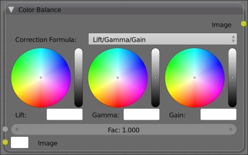
The Color Balance node provides a control that is similar to the RGB Curves node for grading, as shown in following screenshot. The difference is that since this node has a color wheel for each of the Gain/Gamma/Lift components, its easier to manage color-based grading. The same process in the RGB Curves node would be a bit complicated since curves have to be shaped separately for R, G, and B. However, having a curve-based control in the RGB Curves node provides more precision in grading in comparison to the Color Balance node.
The Color Balance and RGB Curves nodes can be used in combination to make flows to have the desired grading control.
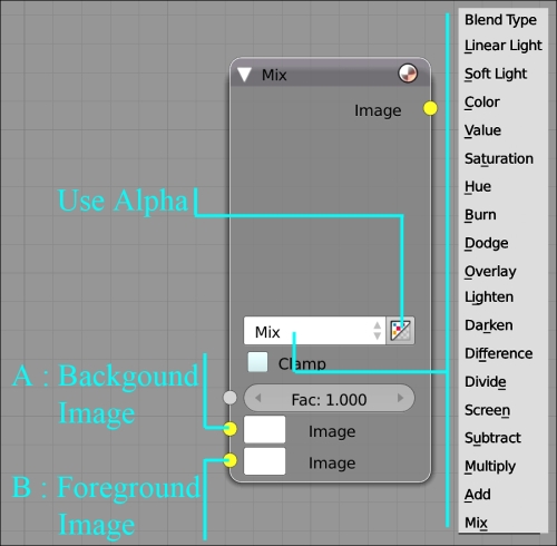
The Mix node blends a base image connected to the top image socket with a second image connected to the bottom image socket based on the selected blending modes, as shown in following screenshot. All individual pixels are mixed based on the mode selected in this node. The Alpha and Z channels are also mixed.
- Mix: In this mode, by using the alpha values, the foreground pixels are placed over the background pixels.
- Add (A+B): In this mode, the pixels from both images are added.
- Subtract (A-B): In this mode, the pixels from the foreground are subtracted from the background.
- Multiply (A*B): This mode results in a darker output than either pixel in most cases (the exception is if any of them is white). This works in a similar way to conventional math multiplication. The behavior is opposite to the Screen mode.
- Screen [1-(1-A)*(1-B)]: In this mode, both images' pixel values are inverted and multiplied by each other and then the result is again inverted. This outputs a brighter result compared to both input pixels in many cases (except if one of the pixels is black). Black pixels do not change the background pixels at all (and vice versa); similarly, white pixels give a white output. This behavior is the opposite of the Multiply mode.
- Overlay {If A<=0.5, then (2*A)*B, else 1-[1-2*(A-0.5)]*(1-B)}: This mode is a combination of the Screen and Multiply modes, and is based on the base color.
- Divide (A/B): In this mode, the background pixels are divided by the foreground pixels. If the foreground is white, the background isn't changed. The darker the foreground, the brighter is the output [division by 0.5 (median gray) is the same as multiplication by 2.0]. If the foreground is black, Blender doesn't alter the background pixels.
- Difference: In this mode, both images are subtracted from one another and the absolute value is displayed as the output. The output value shows the distance between both images: black stands for equal colors and whitefor opposite colors. The result looks a bit strange in many cases. This mode can be used to compare two images, and results in black if they are equal. This mode can also be used to invert the pixels of the base image.
- Darken [Min (A, B)]: This mode results in a smaller pixel value by comparing both image pixels. A completely white pixel does not affect the background at all and a completely black pixel gives a black result.
- Lighten [Max (A, B)]: This mode results in a higher pixel value by comparing both image pixels. A completely black pixel does not alter the image at all and a completely white pixel gives a white result.
- Dodge [A/(1-B)]: This mode brightens the image by using the gradient in the other image. It outputs lighter areas of the image where the gradient is whiter.
- Burn [1-(1-A)/B]: This mode darkens one socket image on the gradient fed to the other image. It outputs darker images.
- Color: In this mode, each pixel is added with its color tint. This can be used to increase the tint of the image.
- Value: In this mode, the RGB values from both images are converted to HSV parameters. Both the pixel values are blended, and the hue and saturation of the base image are combined with the blended value and converted to RGB.
- Saturation: In this mode, the RGB values of both images are converted to HSV parameters. Both pixels saturations are blended, and the hue and value of the base image are combined with the blended saturation and converted to RGB.
- Hue: In this mode, the RGB parameters of both pixels are converted to HSV parameters. Both pixels hues are blended, and the value and saturation of the base image are combined with the blended hue and converted to RGB.
The Use Alpha button of the Mix node instructs the Mix node to use the Alpha channel available in the foreground image. Based on the grayscale information in the alpha channel, the foreground pixels are made transparent to view the background image. The effect of the selected blending mode is thus seen only in the nontransparent foreground pixels. The Alpha channel of the output image is not affected by this option.
The factor input field (Fac) decides the amount of mixing of the bottom socket. A factor of 0.0 does not use the bottom socket, whereas a value of 1.0 makes full use. In Mix mode, 50:50 (0.50) is an even mix between the two, but in Add mode, 0.50 means that only half of the second socket's influence will be applied.
The following screenshot shows outputs from all the described Mix modes without altering the inputs connected to the top and bottom nodes:

An overall gamma correction can be made to the final result using the Gamma node. This correction helps to alter the lighting information in the result.
The Invert node can invert the pixel values in the RGB or Alpha channel based on what is selected in the node. This node comes in handy during masking to invert the alpha channel.
The Hue Correct node is very useful in that it provides unique control to be able to raise or lower the hue, saturation, and value over the visible color spectrum. The following set of screenshots shows the different effects obtained using similar curves in the S and V tabs:

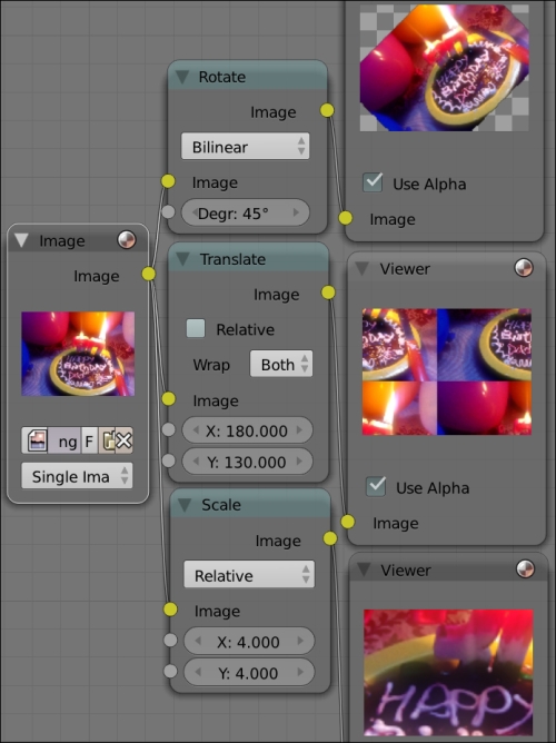
Transformation tools are used to reposition, reorient, or resize the input footage. Blender is equipped with the Rotate, Translate, Scale, Flip, Crop, and Transform nodes as transformation tools. The following screenshot explains the Rotate, Translate, and Scale nodes:
The following screenshot explains the effect of using the Flip node's modes Flip X, Flip Y, and Flip X & Y:

The following screenshot explains how the Crop node can be used to modify an image's boundaries:

The following screenshot explains how to use the Transform node to reposition or reorient an image:
