
Chapter 9. Data for Testing
In the preceding chapter, you saw how to replace one of the two dependencies in data pipeline testing: interfaces to external services. This gets you part of the way to cost-effective testing. This chapter covers how to replace the second dependency mentioned in Chapter 7: external data sources. Instead of using a live data source for testing, you’ll see how to replace it with synthetic data.
There are a lot of neat techniques in this chapter for creating synthetic data, but before you fire up your IDE, it’s important to assess whether replacing a data dependency with synthetic data is the right move. This chapter opens with guidance on how to make the choice between live and synthetic data for testing and the benefits and challenges with each approach.
After this, the remainder of the chapter focuses on different approaches to synthetic data generation. The approach I’ll cover first, manual data generation, is likely one you’ve done when creating a few rows of fake data for unit testing.
The learnings from creating manual data will help you build accurate models for automated data generation, the approach I’ll cover next. You’ll also see how to use data generation libraries to customize data generators so that they provide the data characteristics needed for testing.
Finally, you’ll see how to keep automated data generation models up to date with source data changes by linking data schemas with test generation code. This is a powerful approach that can catch breaking changes as soon as they hit the repo.
The code examples throughout this chapter can be found in the testing directory of the GitHub repo, where you will also find the instructions for setting up a virtual environment and dependencies for running the code.
Working with Live Data
Before getting into creating and working with synthetic data, it’s important to keep in mind that there are times when connecting to live data is a better option. Remember, the goal of testing is to accurately identify bugs. While it is desirable to reduce data dependencies for testing, you don’t want to sacrifice test quality to this goal.
Benefits
Live data, such as from a production environment, can be a rich source that is large in scale and contains a variety of data characteristics. If tests pass using production data, at a minimum you can expect that code changes won’t break production. That’s pretty good.
When working with data where features change unpredictably or with complex data structures that are difficult to create synthetically, working with live data is likely to give you more accurate test results.
Challenges
Corrupting production data with testing activities is a risk you absolutely must avoid when using live data. A former colleague shared a story in which some well-meaning developers at her company added production credentials to unit-test some data pipeline code locally. As a result of running the unit tests, the developers accidentally deleted all the production data in the most important table, in the product’s most central service, resulting in a total outage and major reputational damage.
For this reason, I recommend limiting live data use to read-only. If tests need to create, modify, or delete data, you’re better off using a fake, such as a test database, or a mock.
When testing with live data, additional steps are needed to connect to and authenticate with data sources. Depending on company policies and the type of data involved, it can take time to get access approval and, potentially, additional time to anonymize data for testing purposes. You’ll also need to configure local development environments to access these resources and make sure test code can authenticate and connect.
As an example, I was running a test suite that connected to an Elastic instance in a test environment. If the Elastic connection was down, the code under test would retry for five minutes. Several times I wondered why my pytest session was hanging, ultimately realizing it was retrying the Elastic connection because I forgot to connect or the tunnel went down while testing. In another case, when working with Medicaid data, getting approval to access data could be an endeavor that took weeks or months. With only live data as a testing option, I wouldn’t have been able to meaningfully contribute during that time.
Data privacy is a significant concern when working with production data. Throughout this book, I’ve shared some examples where I’ve worked with medical data, including the ephemeral test environment approach in Chapter 5, which our team used to test against production data due to the strict privacy rules.
In some cases, data may need to be anonymized for testing, where sensitive information such as PII or PHI is removed or obfuscated. If you find yourself in this situation, stop and consult your company’s legal and security teams.
In some cases, the process of anonymizing data removes essential data characteristics needed for accurate testing. If you need to test with anonymized data, compare it to production to ensure that data characteristics are consistent before betting test results on it.
When testing with live data, another thing to consider are the impacts of testing on the resource serving or storing the data. For example, in Figure 8-2 the HoD social media database is processing and serving content for the HoD website. Performance for the website could be impacted with additional load on the database for testing. In these cases, having dedicated read replicas or snapshots available for testing is a good alternative.
A lower-cost alternative to replicas or full snapshots are partial data dumps, providing only the subset of data used for testing over a shortened time period. You can use the test database technique from Chapter 8 and load the database dump using test fixtures.
I’ve worked with systems in which a job is set up to periodically refresh test data, storing a compressed object in cloud storage that is limited to the tables and fields that are of interest for testing. This approach has a smaller storage footprint than a full database dump and does not require database replicas or managing database connections in your unit-testing code. In addition, the refresh cycle kept data up to date with the current state of production.
Working with live data when testing can also increase your bills. Keep this in mind especially when testing data extraction logic. Data pulled from cloud storage will incur costs for egress and object access. When working with third-party data sources, keep in mind how test loads could impact quotas, limits, and costs. For example, I worked on a system that synced data from a content management system (CMS). The CMS had pretty paltry API quotas, so when making code changes, we had to be careful not to exhaust our daily allotment.
Finally, your software development lifecycle may not support live data use. Consider whether you are developing a pipeline that ingests data from a data source maintained by another team at your company. This is an issue I’ve dealt with in the past, where the data source team was trying to meet a deliverable that changed the data schema before the pipeline team had time to implement the schema changes on the ingestion side. The pipeline team was accustomed to using the live data source, but they had to use synthetic data in the interim while adapting to the schema changes. Building in a plan for synthetic data creation can be a good backup strategy so that you won’t be scrambling if a situation like this occurs.
Working with Synthetic Data
I don’t think I’ve ever worked on a data pipeline that didn’t use some form of synthetic data in testing. When I talk about synthetic data, I mean data that has been created manually or through an automated process, as opposed to data that comes directly from a data source such as an API. You’ll have a lot of opportunity to work with synthetic data generation in this chapter.
Benefits
One of the superpowers of synthetic data is that you aren’t limited to the data available in production. That may sound sort of odd: limited by production data? Production data doesn’t always include all the possible cases pipeline code is designed to operate against. With synthetic data, you can ensure that all the important data code paths are tested.
As an example, I worked on a project that got permission from a customer to use their production dataset for testing. While the dataset was large, it didn’t contain the right data characteristics to trigger a performance issue we were debugging in our database queries. This highlights another benefit of synthetic data in that you don’t have to get customer permission.
Another benefit of synthetic data is it can help communicate important data characteristics to other developers. With synthetic data included in your test suite, a new developer can quickly come up to speed without having to gain access to remote systems where live data is stored. You also bypass the kinds of connectivity and authentication issues I mentioned in “Working with Live Data”.
Eliminating connections to data sources saves costs, as you aren’t running queries against a database or accessing cloud storage, and it enables unit tests to be easily added in CI. Later in this chapter, you’ll see how schema-driven data generation and CI testing catch a data pipeline bug before it hits production.
Tip
Generating test data in JSON format will help you share that data across different tools, libraries, and languages. In addition, a lot of data sources provide JSON either natively, in the case of many APIs, or as an export format, such as from a database client.
One of my favorite uses of synthetic data is regression testing, where tests are added to ensure that prior functionality hasn’t been lost. When a data-related bug arises in production, you can reproduce the failure in testing by adding test data that emulates the data that caused the failure. As an aside, if you aren’t already in the practice of reproducing bugs in tests before fixing them, I highly recommend it. Not only will you feel like Sherlock Holmes for isolating the root cause and reproducing the failure, you will be incrementally making your testing more robust.
Finally, the more you can test with synthetic data and unit tests, the less cost and complexity will be associated with testing. Depending on live data or snapshots of live data requires additional cost and overhead for accessing these systems and maintaining snapshots. Even if you can cheaply create a snapshot of data to load into a local database for testing, consider the additional work involved in keeping that development database up to date. In my experience, this often leads to inadvertently testing against stale data and the “it works on my machine” conundrum.
Challenges
While you may find it straightforward to create synthetic data for small-size, low-complexity data sources, this process can become difficult or impossible as data gets larger and more complicated.
It is very easy to go down a rabbit hole1 when creating synthetic data. Fundamentally, you are trying to come up with a model of the source data. When getting started, you’ll naturally gravitate to modeling the most straightforward cases, but things can get complicated as corner cases are encountered that don’t fit the model.
I don’t know about you, but for me, when I’ve gotten most of the way through a problem and uncovered some thorny corner cases, I can easily become enamored with finding a solution. As a matter of fact, this happened to me while trying to come up with examples for this chapter. As a result, I created a model that I wouldn’t use for development but that was very intellectually satisfying to figure out.
I encourage you to resist this temptation. If you find yourself creating a lot of one-off special cases or spending more than a day trying to model a data source, stop and reevaluate whether synthetic data is the right choice. The next section will provide some guidance for this.
Another challenge can be overdoing it on the data model and creating cases that either aren’t relevant or overexercise the code under test. When creating synthetic data, do this side by side with the logic the data will exercise. This will help you home in on the data cases that are relevant to the code under test, keeping you from going overboard with test data generation.
Warning
Be cautious about spending too much time creating synthetic data for data sources that are poorly understood. At worst, you can create invalid data that results in passing tests when the actual data would cause them to fail.
There’s an excellent chance synthetic data will quickly become obsolete and unusable if it requires constant maintenance to stay up to date. Keep in mind the maintenance required when developing synthetic data. You’ll see some techniques in this chapter to automate the data generation process, which will help reduce maintenance needs.
Is Synthetic Data the Right Approach?
Synthetic data can be a real boon to your testing process, but it can be disastrous if it is applied in the wrong situations. In my experience, synthetic data is most valuable when one or more of the following is true:
It models well-characterized, stable data sources.
It is kept up to date automatically or with a minimum of effort.
It is used to test well-bounded logic.
To get a sense of whether synthetic data is right for a given data dependency, consider these questions:
- What are the consequences of inaccuracies in the synthetic data?
Consider the role synthetic data plays in pipeline fidelity and data quality. The more critical testing is in this process, the greater the risk of issues arising from mistakes in synthetic data.
For example, when working with an API data source for a pipeline project, I used both synthetic data and JSON schemas together to ensure that the data was transformed correctly. I used the synthetic data in unit tests to verify handling of different API responses, while the JSON schema was used during runtime to validate that the API response was as expected.
At some point, the API response changed. The unit tests did not catch this change because the synthetic data was not up to date, but the pipeline validation did catch it. Because I was using both unit tests and data validation, as you saw in Chapter 6, the out-of-date synthetic data did not result in a data-quality issue in the pipeline. This is also a good example of how data validation and unit testing complement each other in ensuring pipeline fidelity.
If instead you have a situation where tests are the primary mechanism for ensuring data quality, be absolutely sure that any synthetic data used is accurate. It can be a better idea to use real data in this case.
- How complex is the data source you want to model? How stable is the data format?
Continuing with the API example, this was a good candidate for synthetic data for the following reasons:
There were only a handful of potential responses.
The data structure was consistent across responses.
The API was developed internally.
With a limited number of distinct values to model and a consistent data structure, the API response was low effort to create and maintain. An additional benefit was that the API was developed by another team at the company, so it was possible to share API response schema information. By linking the schema with the synthetic data generation, I could guarantee that the test data was an accurate model.
- What is involved in maintaining the synthetic data? Is the benefit worth the time investment?
If synthetic data is high maintenance, consider how likely it is that it will be kept up over time. Based on my experience, I suspect there is a vast graveyard of well-intentioned synthetic data that fell by the wayside due to lack of maintenance.
For the rest of the chapter, you’ll see different techniques for creating synthetic data to test parts of the HoD survey pipeline from Chapter 7, repeated here in Figure 9-1.
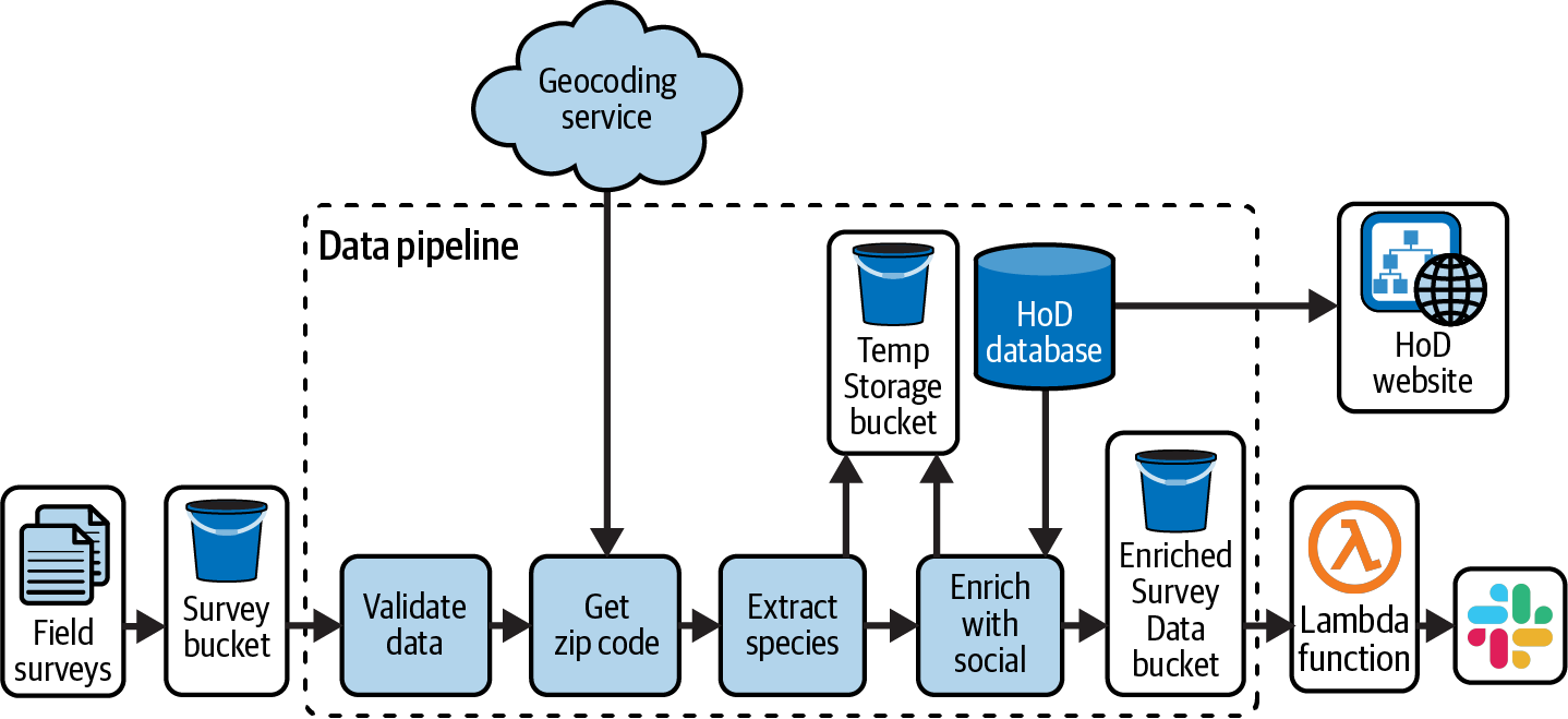
Figure 9-1. HoD batch survey pipeline
The synthetic data approaches presented are based on building some simple models of live data samples. There are more advanced techniques that I won’t cover, such as creating data through statistical processes, artificial intelligence, or other algorithmic means. There are entire products and services that focus on creating synthetic data, as well as books and journal articles on the topic.
The data you’ll see modeled in the rest of the chapter is the source data for the survey pipeline, the Field survey data stored in the Survey bucket in Figure 9-1. An example of the survey data is shown in Table 9-1 to provide a sense of the data characteristics.
| User | Location | Image files | Description | Count |
|---|---|---|---|---|
| [email protected] | (45.2341, 121.2351) | Several lesser goldfinches in the yard today. | 5 | |
| [email protected] | (27.9659, 82.8001) | s3://bird-2345/34541.jpeg | Breezy morning, overcast. Saw a black-crowned night heron on the intercoastal waterway. | 1 |
| [email protected] | (45.4348, 123.9460) | s3://bird-1243/09731.jpeg, s3://bird-1243/48195.jpeg | Walked over to the heron rookery this afternoon and saw some great blue herons. | 3 |
The survey dataset contains a row for each sighting recorded by a user of the bird survey app. This includes the user’s email and location and a freeform description. Users can attach pictures to each sighting, which are stored by the survey app in a cloud storage bucket, the links to which are listed in the “Image files” column. Users can also provide an approximate count of the number of birds sighted.
The survey data is transformed in the “Extract species” step in Figure 9-1. The transformation looks for specific heron species within the Description field and creates a new column, Species, that contains the matching species, or null if no match is found. Table 9-2 shows the results of the survey data in Table 9-1 after it is transformed by the “Extract species” step.
| User | Location | Image files | Description | Species | Count |
|---|---|---|---|---|---|
| [email protected] | (45.2341, 121.2351) | Several lesser goldfinches in the yard today. | 5 | ||
| [email protected] | (27.9659, 82.8001) | s3://bird-2345/34541.jpeg | Breezy morning, overcast. Saw a black-crowned night heron on the intercoastal waterway. | night heron | 1 |
| [email protected] | (45.4348, 123.9460) | s3://bird-1243/09731.jpeg, s3://bird-1243/48195.jpeg | Walked over to the heron rookery this afternoon and saw some great blue herons. | great blue heron | 3 |
This transformation is performed by the apply_species_label method, as depicted in the following code, which you can find in transform.py. You’ll run this code later as part of the unit test; for now, just get a sense of how it works:
species_list=["night heron","great blue heron","gray heron","whistling heron"]defapply_species_label(species_list,df):species_regex=f".*('|'.join(species_list)}).*"return(df.withColumn("description_lower",f.lower('description')).withColumn("species",f.regexp_extract('description_lower',species_regex,1)).drop("description_lower"))
To extract the species label, a list of species, species_list, is combined into a regular expression (regex). This regex is applied to a lowercase version of the description column, description_lower. The first substring to match an element in species_list is extracted as the species column. Once the species has been determined, the description_lower column is dropped as it is not needed anymore.
Manual Data Generation
When you’ve decided to use synthetic data, manual data generation is the place to start. It may also be the place to end depending on the data you are modeling and the tests that use it.
In general, manual data generation is best suited when the scope of both the test and the data is small and well defined. Anytime you have to modify code or test collateral, there are opportunities for bugs, in addition to the staleness problem I mentioned earlier. Keeping the scope limited when using manual data will minimize these undesirable states.
Manual data is a good approach if the following statements describe your intentions:
The tests you need to run are limited in scope, such as validating a handful of possible API responses.
The data you are modeling changes infrequently.
You need a small number (let’s say 10 or fewer) of attributes.
You aren’t trying to validate the handling of wide, sparse datasets.
Even if an automated data generation process is the end goal, curating a small dataset by hand will help you get to know the data characteristics and think through the cases that need to be modeled.
Let’s dive into creating some test data for testing the apply_species_label. This is a good place to use manual data generation; you need a few rows of data to validate that the transformation is working properly, but because it’s early in the development process, bugs are likely. Rather than investing the time to set up synthetic data generation at this point, it’s better to focus on iterating quickly with simple tests.
Before moving on, think about some test cases you’d want to create for apply_species_label. Notice how you start building a mental model of possible values for the description field and how you expect apply_species_label to perform in those cases. Oftentimes I find bugs in my code just thinking through different possible test cases before writing any test code.
Here is a snippet of some manually generated test data for apply_species_label, showing just the description field for brevity. The full code is in the create_test_data function in manual_example.py:
fake_data=[{"description":"there was a night heron",...},{"description":"",...},{"description":"there was a heron",...}]
There are a few cases represented in this test data. There’s a case where an entry in the species_list is part of the description, "there was a night heron", as well as some edge cases of an empty description and a description that partially matches entries in the species_list.
This provides the input data for the unit test, but you also need to create the expected output for each case. When testing apply_species_label, make sure the species field is accurately extracted and that no other fields are modified. For now, let’s focus on validating the species field using the following expected results:
expected=[{"user":"[email protected]","species":"night heron"},{"user":"[email protected]","species":""},{"user":"[email protected]","species":""},]
To see these test cases run, set up a local development environment, as described in the testing README. To activate the virtual environment, try running the test as follows:
(my_venv)$ cd testing
(my_venv)$ pytest -v test_transform.py::test_transform_manual
You may notice that the test takes several seconds to run. This is due to setting up the fixture spark_context, which creates a new Spark session when the testing session begins. Once the test completes, you should see something like the following:
collected 1 item
test_transform.py::test_transform_manual PASSED
To see what a failing test looks like, set description=None for this line of synthetic data in manual_example.py:
"user":"[email protected]","location":"45.12431, 121.12453","img_files":[],"description":None,"count":10,
When you run the test again, you’ll see a failing case:
>          assert result_case[0]['species'] == species
E          AssertionError: assert None == ''
The test code has some print statements to help debug which test cases failed. Here you can see the case where description in the input data is set to None, causing the test failure:
Result: [{. . . 'description': None, 'user': '[email protected]',
                'species': None}]
Expected: {'user': '[email protected]', 'species': ''}
Manual data generation doesn’t necessarily mean you have to handcode test cases. For example, one of the synthetic datasets I’ve used was manually curated by gathering a few representative rows of data from a test environment database. You may also be able to use free datasets as a source of test data, such as those from NASA.
Automated Data Generation
If all data was well defined, small in scope, and static, you probably wouldn’t be reading this book because there would be little need for data pipelines. When you have more sophisticated testing needs, automated data generation can be a better choice than trying to manually curate test data. Consider automation when you need the following:
A significant number of fields for testing (wide datasets)
A large dataset (i.e., load testing)
A desire and ability to tie data generation to specs, such as data models or schemas
Data generation based on a distribution of values
Consider that the pipeline in Figure 9-1 operates on a batch of survey data. While some enthusiasts may be surveying birds year-round, it’s likely that there will be larger batches at certain times of the year. In addition to batch size, there is also variation in the description field contents. Some users may rarely use the description field, while others may use it extensively but never mention any particular species. This section illustrates a few ways to automate data creation for these examples.
Synthetic Data Libraries
One approach to creating synthetic data is to use a library. Faker is a Python library that generates synthetic data, from primitive types such as boolean and integer to more sophisticated data such as sentences, color, and phone numbers, to name a few. If you don’t find what you need among the standard and community providers, try creating your own. A provider is the Faker term for a fake data generator.
The method basic_fake_data in faker_example.py shows how to use Faker to create synthetic data to test apply_species_label. This example uses several Faker built-in providers, including email, latitude and longitude, filepath, and words:
defbasic_fake_data():fake=Faker()fake_data={"user":fake.(),"location":fake.local_latlng(),"img_files":[f"s3://bucket-name{fake.file_path(depth=2)}"],"description":f"{' '.join(fake.words(nb=10))}","count":random.randint(0,20),}fork,vinfake_data.items():(k,":",v)
Try running this code by opening a Python terminal in the virtual environment in the testing directory. Keep in mind that the results are random; the results printed here will be different from what you see when running the fake data generators:
(my_venv)$cdtesting(my_venv)$python...>>>fromfaker_exampleimportbasic_fake_data>>>basic_fake_data()user:lindseyanderson@example.orglocation:('41.47892','-87.45476','Schererville','US','America/Chicago')img_files:['s3://bucket-name/quality/today/activity.txt']description:anothervoicerepresentworkauthoritydaughterbestdreamnamemeetingcount:13
Tip
While developing test data with a generator, it’s a good idea to log the test cases so that you can review them for unexpected results.
Looking at basic_fake_data, notice that there isn’t a list of different test cases, as there is with the manual data generation approach. Instead, fake_data is a dictionary that can be created any number of times to generate new test cases. In the terminal, call basic_fake_data again and you’ll see that a new set of synthetic data is created:
>>>basic_fake_data()user:wilsonbront@example.netlocation:('39.78504','-85.76942','Greenfield','US','America/Indiana/Indianapolis')img_files:['s3://bucket-name/sure/ground/establish.pptx']description:budgetpandaanimalactvisitagentimportanthalfrespondstuffcount:8
Another benefit of this automated approach is that you don’t need to manually update all the test cases if there is a change to the data schema. Instead, you just update the Faker definitions. For example, let’s say the user field changes from an email address to a UUID. In the basic_fake_data function, change fake.email() to fake.uuid4(). To see this change in the terminal, you’ll need to quit and restart Python and then reimport the module. Now when you run basic_fake_data, you can see the UUID instead of the email for the user field:
(my_venv)$python>>>fromfaker_exampleimportbasic_fake_data>>>basic_fake_data()user:b7e61421-b7e5-4266-bc3f-2e3575358d32location:('41.47892','-87.45476','Schererville','US','America/Chicago')img_files:['s3://bucket-name/quality/today/activity.txt']description:anothervoicerepresentworkauthoritydaughterbestdreamnamemeetingcount:13
Warning
When using a library to help generate synthetic data, make sure to validate your assumptions about the data being created.
For example, while working on this chapter, I realized the Faker email provider does not generate unique results when creating more than 1,000 test cases. While libraries like Faker can help streamline your code, make sure to validate the data they produce.
Customizing generated data
When using synthetic data providers such as Faker, it may be necessary to tweak the values they provide out of the box to match the data you need to create. In this example, the description field needs to occasionally include elements from the species_list.
The DescriptionProvider class in faker_example.py implements a customer Faker provider, with a description method that adds this functionality:
defdescription(self):species=fake.words(ext_word_list=util.species_list,nb=randint(0,1))word_list=fake.words(nb=10)index=randint(0,len(word_list)-1)description=' '.join(word_list[0:index]+species+word_list[index+1:])
species will be either an entry from species_list or an empty list. Note that in this case, word refers to a single entry in the list provided to ext_word_list. species is concatenated with additional words to create a sentence, emulating what a user might submit in the bird survey.
Continuing with the Python terminal opened earlier, you can generate some descriptions using this new provider:
>>>fromfaker_exampleimportDescriptionProvider>>>fromfakerimportFaker>>>fake=Faker()>>>fake.add_provider(DescriptionProvider)>>>fake.description()'leave your stop fast sport can company turn degree'>>>fake.description()'card base environmental very computer seek view skin assume'>>>fake.description()'choose sense night studentnight herontwo it item mouth clearly'
Something to keep in mind about this approach is the use of randint(0,1) for choosing whether to include the species in the description. You could call fake.description() several times and never get a description that has a species.
Tip
To use Faker in a unit-testing scenario where you want to create the same data each time, provide a seed to the generator. In the description generator from this example, make sure to seed the random number generator as well. Consider logging the seed; if a test is flaky, you can re-create the test case with the logged seed.
Assuming you are generating a large number of cases, this shouldn’t be a problem.2 If there are specific cases that must be included in a test suite and you cannot guarantee the data generator will be called enough times to exercise all the cases, you would be better served by adding some manual cases:
defcreate_test_data_with_manual(length):data,expected=manual_example.create_test_data()auto_data,auto_expected=create_test_data(length)return(data+auto_data,expected+auto_expected)
Distributing cases in test data
If you have multiple cases to represent and want to control their distribution in the test data, apply weights when generating test data. In Spark, RandomRDDs can be used to generate randomly distributed data. Continuing the Faker example, try combining a customized description provider with random.choices to choose how the cases should be distributed.
At this point, the description provider provides two cases: a description with a species and a description without a species. There is no empty string, there are no partial species matches, and there is no string that has a full or partial species name without any other text.
These cases are included in the Faker provider, as shown in description_distribution in faker_example.py:
defdescription_distribution(self):...cases=['',species,species_part,words_only,with_species,with_part]weights=[10,2,3,5,6,7]returnchoices(cases,weights=weights)
In this provider, there are cases representing the possible description values, which include an empty description and the cases in Table 9-3.
| Case | Description example |
|---|---|
species | "night heron" |
species_part | "heron" |
words_only | "participant statement suggest country guess book science" |
with_species | "night heron participant statement suggest country guess book science" |
with_part | "heron participant statement suggest country guess book science" |
The weights in description_distribution indicate how frequently a given case occurs. In this example, the most common occurrence is an empty string. This might reflect the actual survey data, since many users could choose to include images instead of a description. You could also intentionally skew the weights to stress certain scenarios. For example, the bird survey app could add a speech-to-text feature that populates the description field. With the overhead of typing removed, users might start adding more descriptions.
At this point, you have a description provider that will provide a distribution of all possible cases. Just as in the manual case, generate the expected results for testing at the time the test data is generated. The description_distribution_expected method in faker_example.py returns both the generated description and the expected values of the species field. I’m omitting the code here for brevity, but when reviewing it, consider how to write generator code to return the expected results along with the generated test data.
While synthetic data libraries can be handy, there are times when they can be overkill too. You can create data generators using Python standard libraries.
For example, let’s say there is a unique ID attached to every Survey Data record with the format bird-surv-DDDDD where D is a digit. Using Python’s string and random libraries, it’s possible to create a data generator for this, as shown in generate_id in faker_example.py:
fromstringimportdigitsdefgenerate_id():id_values=random.sample(digits,5)returnf"bird-surv-{''.join(id_values)}"
create_test_data_ids illustrates using this function to generate IDs, similar to how the Faker providers are called:
defcreate_test_data_ids(length=10):mock_data=[]for_inrange(length):mock_data.append({"id":generate_id(),"user":fake.(),...
To give this a test drive, return to the terminal where you loaded DescriptionProvider:
>>importutil>>fromfaker_exampleimportcreate_test_data_ids>>create_test_data_ids()[{'id':'bird-surv-26378','user':'[email protected]','location':...
Schema-Driven Generation
So far, you’ve seen how to create a synthetic data generator that can mimic the size and distribution of values from a source dataset. The data generation happens at test time, so there is no data to maintain or store. While this provides some benefits over manual data, there’s an outstanding question of what happens when the source dataset changes. How will you know the synthetic data generator is out of date?
As described in Chapter 4, schemas are a powerful tool for data validation. Schemas are also useful when creating test data; linking the data generation process to schemas will help you track changes in source data. In this section, you’ll see how to link the automated data generation techniques in “Synthetic Data Libraries” to a schema to further automate test data generation.
Ideally you have access to explicit data schemas, meaning definitions that are used as part of the data pipeline to describe the data being processed. These could be represented as JSON or Spark schemas. If explicit schemas aren’t available, you can extract schemas from a data sample for testing. mock_from_schema.py provides an example of how to do this for a Spark DataFrame:
defcreate_schema_and_mock_spark(filename,length=1):withopen(filename)asf:sample_data=json.load(f)df=spark.sparkContextparallelize(sample_data).toDF()returngenerate_data(df.schema,length)
With the DataFrame loaded, df.schema gives you the schema, which can be used for the data generation technique in this section:
StructType(List(StructField(count,LongType,true)StructField(description,StringType,true)StructField(img_files,ArrayType(StringType,true),true)StructField(location,ArrayType(StringType,true),true)StructField(user,StringType,true)))
A JSON version of the schema can be obtained by calling df.schema.json().
When working with Pandas, you can extract a JSON schema using build_table_schema, but keep in mind that the schema inference provided by Spark gives a richer view of the underlying data types. Consider this Pandas schema generated from the same sample data as that used for the preceding Spark schema:
'fields':[{'name':'index','type':'integer'},{'name':'user','type':'string'},{'name':'location','type':'string'},{'name':'img_files','type':'string'},{'name':'description','type':'string'},{'name':'count','type':'integer'}],
Notice that img_files and location are listed as string types, while their contents are an array of strings. There is also no nullable information.
Mapping data generation to schemas
The way to drive synthetic data generation from schemas is to map the schema columns and data types to data generators (such as Faker providers) that represent the types described in the schema.3
For fields where you just want to create data that is of the data type defined in the schema, you can create a map from the field type to a data generator, as illustrated in mock_from_schema.py in DYNAMIC_GENERAL_FIELDS:
DYNAMIC_GENERAL_FIELDS={StringType():lambda:fake.word(),LongType():lambda:fake.random.randint(),ArrayType(StringType()):lambda:[fake.word()foriinrange(fake.random.randint(0,5))]}
For cases where you want to create more specific values than just the data type, you can create a separate map that considers both the column type and the name, as with the DYNAMIC_NAMED_FIELDS map:
DYNAMIC_NAMED_FIELDS={("count",LongType()):lambda:fake.random.randint(0,20),("description",StringType()):lambda:fake.description_only(),("user",StringType()):lambda:fake.(),}
Tip
The column-based data generation approach in this section is really helpful for wide datasets. You can simply add new entries to the DYNAMIC_GENERAL_FIELDS map or the DYNAMIC_NAMED_FIELDS map for the columns you want to generate data for.
Using these maps, you can set up a data generator based on the Spark schema. First, determine which data generator to return for a given column name and data type. Raising an exception if a column isn’t found in the maps will highlight when the data generation code needs to be updated:
defget_value(name,datatype):ifnamein[t[0]fortinDYNAMIC_NAMED_FIELDS]:value=DYNAMIC_NAMED_FIELDS[(name,datatype)]()returnvalueifdatatypeinDYNAMIC_GENERAL_FIELDS:returnDYNAMIC_GENERAL_FIELDS.get(datatype)()raiseDataGenerationError(f"No match for{name},{datatype}")
Another note about get_value is that the DYNAMIC_NAMED_FIELDS map is searched for a name match. If there is a name match but the data type does not match, value = DYNAMIC_NAMED_FIELDS[(name, datatype)]() will throw a KeyError. This is intentional; if the test fails due to this exception, it will help you track breaking schema changes. With the ability to get a generated data value for each column, you can create a DataFrame of test data by running a map over the fields specified in the schema:
defgenerate_data(schema,length=1):gen_samples=[]for_inrange(length):gen_samples.append(tuple(map(lambdafield:get_value(field.name,field.dataType),schema.fields)))returnspark.createDataFrame(gen_samples,schema)
Let’s take a look at what the schema-based data generation looks like. A schema for the survey data is available in schemas.py:
$cdtesting$python>>>fromschemasimportsurvey_data>>>frommock_from_schemaimportgenerate_data>>>df=generate_data(survey_data,10)>>>df.show(10,False)
Table 9-4 illustrates some of the generated data for the description and user fields.
| Count | Description | User |
|---|---|---|
13 | "[email protected]" | |
5 | "heron" | |
6 | "sure and same culture design gray heron fire use whom sell last" | "[email protected]" |
0 | "cold beat threat keep money speech worker reach everyone brother" | "[email protected]" |
Now that schema-based mock generation is working, you can add the expected data generation. This is a bit trickier than the earlier Faker case in “Synthetic Data Libraries”. In that case, the entire row of data is being generated at once. With the schema-based generation, you’re creating each column of data individually. To keep track of the expected values, you can add some state that persists over the course of generating each row. generate_data_expected in mock_from_schema.py shows this updated approach.
To see the schema-driven data generation in action you can run the test from the virtualenv:
(my_venv)$ cd testing
(my_venv)$ pytest -v -k test_transform_schema -s
Table 9-5 shows example description and species values returned by apply_species_label during the test with the schema-generated data.
| User | Description | Species |
|---|---|---|
"[email protected]" | ||
"[email protected]" | "change you bag among protect executive play none machine spring night heron" | "night heron" |
"[email protected]" | "heron" | |
"[email protected]" | "himself suddenly industry chance sister whistling heron economic teacher early run name" | "whistling heron" |
Example: catching schema change impacts with CI tests
To really get a sense of how much more coverage you get by linking synthetic data generation to production schemas, let’s take a look at what happens if there is a schema change.
Let’s assume that the description field changes from a string to an array of strings. The survey_data schema gets updated to reflect the change:
T.StructField("description",T.ArrayType(T.StringType(),True),True)
A merge request is created for the updated schema, kicking off CI testing. Because you’ve replaced the Survey Data bucket dependency in Figure 9-1 with synthetic data, test_transform_schema can be included in a CI test suite. This test fails with the following error:
mock_from_schema.DataGenerationError: No field mapping found for description,
      ArrayType(StringType,true)
This failure highlights that the synthetic data is broken as a result of this schema change. The code for apply_species_label will also be broken, but the manual and Faker-generated data tests would not have caught this because the schema wasn’t applied to the test data.
Had this test not caught this failure, the next place it would have shown up is in a pipeline fault, ideally a validation error that halted the pipeline, preventing bad data from being ingested. Instead of identifying the error in a controlled environment like unit tests, this schema change could have resulted in an incident.
Property-Based Testing
A data generation and testing methodology wrapped in one, property-based testing starts from the assertions in a test and works backward to generate data inputs that break those assertions. The Hypothesis library provides different data generation strategies that you can apply when running unit tests. There is some similarity here to how Faker providers generate data.
Property-based testing is really a different way of thinking about tests. Your test assertions serve the functions of both validating the code under test and providing property-based testing frameworks with criteria for coming up with test cases. Done well, test assertions are also great documentation for other developers.
For example, Hypothesis will generate new test cases in an attempt to cause the test to fail and then present the minimum version of that test case for inspection. If you’re new to property-based testing, the Hypothesis team provides a nice introduction to the topic.
Property-based testing is a specialized approach you can use when a method’s requirements can be expressed in mathematical terms. It’s not likely to be a go-to approach for most of your data pipeline tests, but when it’s relevant it is really effective. Giving a property-based testing framework the job of coming up with the data corner cases frees you up to focus on the big picture.
Recall the “Validate data” step in the survey data pipeline in Figure 9-1. Part of this data validation is checking that the user field is a valid email address. Now, there are already a lot of ways to validate an email address, but for the sake of illustration, let’s suppose the HoD team started with this method in test_validation.py:
defis_valid_email(sample):try:assert'@'insampleassertsample.endswith(".com")returnTrueexceptAssertionError:returnFalse
Here is a test using the hypothesis email strategy for is_valid_email:
fromhypothesisimportgivenfromhypothesisimportstrategiesasst@given(st.emails())deftest_is_valid_email(emails):assertis_valid_email(emails)
The given decorator marks a test as using hypothesis, and the arguments to this decorator are the strategies to use as the fixtures to the test. The emails strategy generates valid email addresses.
Try running this test and you’ll see how quickly Hypothesis comes up with a failing case:
(my_env)$pytest-v-ktest_is_valid_email>assertis_valid_email(emails)EAssertionError:assertFalseE+whereFalse=is_valid_email('[email protected]')test_validation.py:17:AssertionError------------Hypothesis--------------Falsifyingexample:test_is_valid_email(emails='[email protected]',)
hypothesis prints the test case it generated that failed the check, providing important information that you can use to either fix the underlying code or modify the Hypothesis strategy if the falsifying example is not valid. In this case, the assertion that an email address needs to end in .com is what caused the failure.
Spending a lot of time customizing a strategy to provide the right test cases can be a sign that property-based testing isn’t the right approach. Similar to how you can end up down a rabbit hole when creating synthetic data models, keep an eye on the complexity of property-based strategies.
Summary
There are a lot of advantages to using synthetic data when testing data pipelines: reducing cost and test environment complexity by eliminating data dependencies, enabling CI testing, improving team velocity by baking important data characteristics directly into the codebase, and empowering you to tailor test data to testing needs.
Remember, accurate testing and minimal maintenance is the goal. While there are many benefits of synthetic data, it’s not always the right choice, particularly if data is poorly understood, variable, or complex. You may be able to assess this right off the bat, or you may uncover complexities as you start trying to model the source data.
If you need to use live data for testing, consider read replicas or snapshots to reduce load on shared resources. You can also use the test database method covered in Chapter 8 to load partial database dumps for testing. If sensitive information is a concern when using live data, get in touch with the security and legal teams at your company to determine how to proceed.
Manual data is the place to start when creating synthetic data for testing, even if you plan to use an automated approach. Handcrafting a few rows of data to test logic and data transformations will help you iterate quickly to refine code and will provide a sense of the contours of the data and your testing needs. This will help you come up with good models when creating automated data generation processes.
For small amounts of relatively static data, manual data generation may be all you need. When you need synthetic data at scale, automated techniques can generate any number of rows or columns of data while minimizing the maintenance burden with data generators.
You may find that Python’s standard library has the tools needed for creating synthetic data models, as you saw with the strings and random libraries. Another option is data generation libraries like Faker, which give you a large selection of off-the-shelf data providers.
A powerful way to keep synthetic data models up to date with source data is by linking data schemas to data generation. As you saw in the example, this approach can help detect breaking schema changes as soon as they trigger CI tests. In addition, the map-based generation technique can be easily extended to include various data types and shapes.
If you have methods that lend themselves to property-based testing, it can be a helpful tool to offload test data generation responsibilities. Be sure the property-based strategies create test cases that accurately represent your data to avoid under- or over-testing code.
The last pillar of cost-effective design is observability, starting with logging in Chapter 10 and monitoring in Chapter 11. Without good logging and monitoring, the work you’ve put into design resources, code, and testing will fall short of giving you the best bang for your buck. Observability is such a critical part of cost-effective practices that I nearly made it the first chapter in the book!
1 Carroll, Lewis. Alice’s Adventures in Wonderland, Chapter 1.
2 Determining the number of times to generate data to cover a specific number of cases is the topic of the Coupon collector’s problem. Refer to this to determine how many times you need to sample to hit all cases.
3 The approach in this section is based on a Scala solution.