Identifying Scaling Opportunities

Before getting into the business of how to scale, let’s start by determining where you have opportunities to scale data pipelines. Two main ingredients are required for scaling: variability and metrics.

Variability is what gives you the opportunity to scale. Without this, you have static resource use. If I’m hiking on a hot, sunny day, I’m not going to bring layers;¹ I know I’m going to be warm the entire time regardless of how strenuous the hike is or how quickly I do it. Variable conditions are what lead me to add or remove layers. In data pipelines, variation in operation and workload is where scaling opportunities abound.

Metrics are what you use to identify when to scale. Memory use increases as a large batch of data is processed, indicating that more resources are needed. The time of day when the largest jobs are processed has passed. Data volumes decrease, as does CPU utilization, providing an opportunity to scale in to reduce costs.

Variation in Data Pipelines

You can think about variation in data pipelines in terms of pipeline operation and data workload. Pipeline operation refers to how frequently the pipeline processes data. Data workload encompasses changes in data volume and complexity. Figure 2-1 illustrates a baseline case of constant operation and constant workload. In a data pipeline, this could be a streaming system that monitors temperature every few seconds. There isn’t an opportunity to scale here, because nothing is changing over time.

Figure 2-1. Constant workload, constant operation

As data workload and pipeline operation move from constant to variable, you have more opportunities to scale for cost and performance. You can scale in a pipeline with variable operation to save costs when there are no or few active jobs, as illustrated in Figure 2-2. This includes batch pipelines and streaming pipelines that process data intermittently.

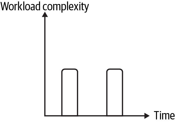
Figure 2-2. Constant workload, variable operation

A caveat in the “constant workload, variable operation” case is differentiating between scaling and triggering intermittent pipeline jobs. In the batch pipeline in Chapter 1, jobs are triggered, either on a schedule or by an external event. In another example, I worked on a pipeline that ran jobs during certain time periods. Our pipeline scaled down to a minimum set of resources outside of these time periods and scaled up when jobs were expected. Both examples have the characteristics of Figure 2-2, but one uses scaling while the other uses triggering to bring necessary resources online.

Data workload variability gives you the opportunity to service large workloads by scaling out, while also saving costs by scaling in when processing small workloads. Batch pipelines where data workloads fluctuate and stream processing with variable data loads are good candidates for scaling based on workload. Figure 2-3 shows a profile of a pipeline with variable workload and constant operation.

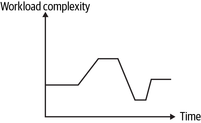
Figure 2-3. Variable workload, constant operation

You have the most scaling opportunity in pipelines that have variation in both data workload and pipeline operation, as depicted in Figure 2-4. This is where cloud billing models really shine, letting you reduce costs for smaller loads without sacrificing performance for larger loads.

Pipelines with fluctuating workloads fall into this category. Examples include streaming pipelines that have bursty behavior, processing little or constant data interspersed with spikes, and ad hoc batch pipelines.

Figure 2-4. Variable workload, variable operation

These examples show variation in a system-level setting. There is also variation in how different workloads are processed within the data pipeline.

Some stages in a pipeline may be computationally intensive, requiring more compute resources, whereas other stages might not need as much firepower. You can scale in resources as data progresses past the computationally intensive stages, ensuring that you are spending for the scaled-out resources only for the duration of data processing that requires them.²

Tip

Be sure to investigate scaling when doing lift and shift migrations, where you move a workload into the cloud without resizing or redesigning it. This can be a very expensive proposition if you don’t take advantage of cloud elasticity to reduce costs.

Additionally, pipeline stage resource needs can vary from job to job, providing another opportunity for scaling. “Pipeline Scaling Example” includes examples of these types of variability.

Pipeline Scaling Example

Recall the HoD batch pipeline from Chapter 1, which processes bird survey data on a biweekly basis. The data volume chart is repeated in Figure 2-5 for reference.

Figure 2-5. Biweekly data workload

Now let’s review the scalability questions.

How does pipeline operation change over time? Pipeline operation is variable, running only every two weeks or perhaps ad hoc as needed.

How does data workload vary? The histogram shows that the data volume varies seasonally.

The survey data isn’t the only data source, however. Shown in Figure 1-3 and repeated in Figure 2-6, the pipeline enriches survey data with the social media data from the HoD platform. The data volume from the social media source is unpredictable; it depends on what birds and locations are in the survey data being processed and those that are present in the HoD database.

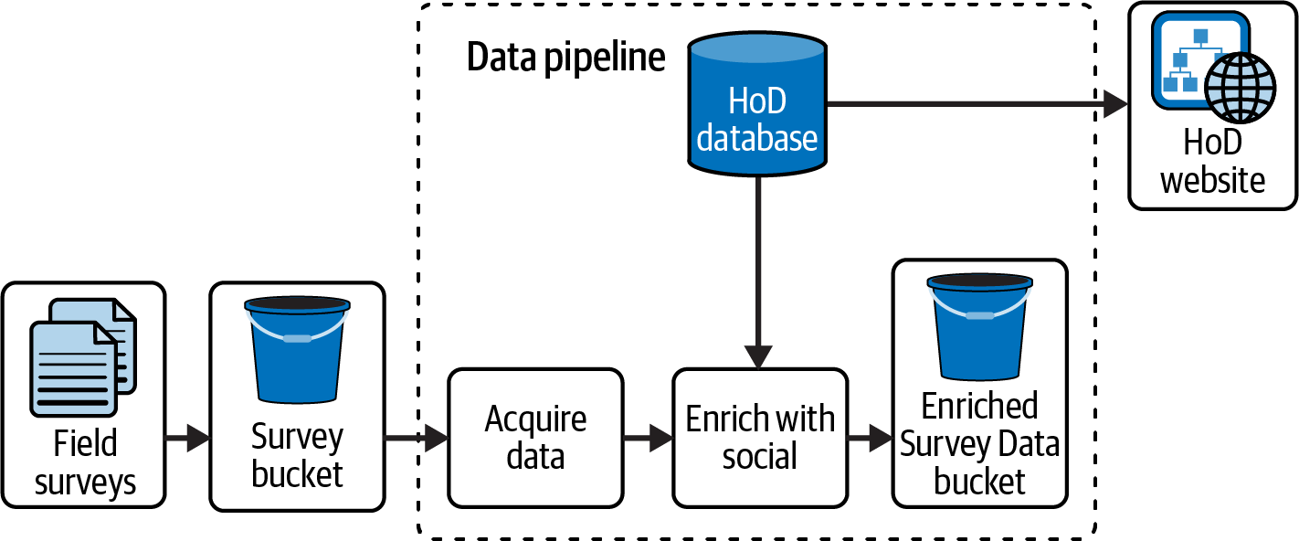
Figure 2-6. HoD batch pipeline

Revisiting the question of how data workload varies, both the survey data and the social data have varying volumes.

How does variation in data workload or operation impact resource needs? Based on the benchmarking results for this pipeline in Chapter 1, you know that memory needs are elastic depending on the data workload. There’s also the biweekly schedule to consider. Most of the time, you won’t need to have resources available—just when a job runs.

The overlap between the survey data and the social media data also impacts resource needs. The “Enrich with social” step could be resource intensive if there is significant overlap in the data sources, or it could require very few resources if there are no matches.

How do you know that resource needs are changing? Good question. To answer this, let’s first take a look at how resource needs change as data moves through the HoD pipeline.

Thinking back to variation within the pipeline, the “Enrich with social” step in Figure 2-6 is likely to require more resources than the “Acquire data” step, owing to the merge. Resources can be scaled out at the beginning of “Enrich with social” and scaled back in when the merge is finished. Figure 2-7 illustrates this idea, where the filled background for “Enrich with social” indicates higher resource needs than the white background for “Acquire data.”

Figure 2-7. Scaling resources per stage. The filled box indicates higher resource needs.

Another source of variation is the unknown overlap between survey data and social media data, which will impact the resource needs of “Enrich with social.”

Figure 2-8 shows this scenario, with the relationship between the survey data and the social data shown on the left and the corresponding resource needs of the “Enrich with social” step on the right. The darker the “Enrich with social” background is, the more resources are needed to merge the data.

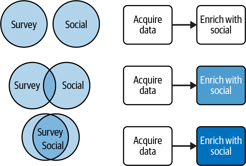
Figure 2-8. Different resource needs across pipeline jobs

To summarize, resource needs can change in the HoD pipeline based on the stage of processing and data characteristics. So how do you know that resource needs are changing?

Based on the benchmarking for this pipeline in Chapter 1, you know this is a memory-heavy process. As data size and survey–social overlap increase, so will memory use. With this in mind, you can look for sustained increases in memory use as an indication that more resources are needed. Conversely, a reduction in memory use can indicate that fewer resources are needed, providing an opportunity to save costs by scaling in.

With all the scaling questions answered, let’s work out a scaling plan.

The biggest bang for the buck comes from allocating compute at the time a job is initiated, as opposed to a 24-7 deployment. Once the job completes, the compute resources can be released.

In a cluster compute environment such as AWS EMR, you can launch a cluster at the time a job is initiated and set it to terminate once the job is finished. If you’re working in Kubernetes, you may have to keep a minimum deployment running, as horizontal pod autoscaling (HPA) does not support scaling to zero at the time of this writing, though it is in the works.

With the on-demand deployment model in mind, the next question is how many compute resources are needed to run the jobs. The variation in workload and the fluctuating resource needs of the “Enrich with social” step indicate there are opportunities to scale.

Combining the information about data volume from Figure 2-5 and the resource needs based on dataset overlap in Figure 2-8, you can see two extreme cases: low-volume survey data and no overlap, and high-volume survey data and high overlap. Benchmarking these cases will provide a starting point for minimum and maximum resource needs.

Let’s say benchmarking shows you need three workers for the low-volume, no-overlap case and 10 workers for the high-volume, high-overlap case. This gives you a starting point for your minimum bound (no fewer than three workers) and maximum bound (no more than 10 workers).

Note that I said these min/max values are a starting point. Like right-sizing from Chapter 1, tuning scaling bounds is an iterative process. When starting out, pad your min and max boundaries. This will ensure that you don’t sacrifice performance and reliability by under-provisioning. Monitor resource utilization and pipeline performance to see whether you can reduce these values.

Designing for Scaling

Before I got into technology, I aspired to be a jazz musician. A characteristic of jazz music is improvisation, in which musicians spontaneously create melodies over the chord changes of a song. I remember diligently learning which scales corresponded to various chord changes as I learned to improvise.

During a lesson, I was shocked when my teacher asked me whether I knew my scales. “Of course!” I replied, and promptly busted out my repertoire of notes. He shook his head and said, “Well, why don’t you use them?” It only then occurred to me that simply knowing what notes to play wasn’t enough; I had to intentionally incorporate them into my playing.

Similarly, just because you are adding or removing compute capacity doesn’t mean your pipeline will take advantage of this elasticity. You need to design to support scaling.

A key design consideration for supporting horizontal scaling is using distributed data processing engines such as Spark, Presto, and Dask. These engines are designed to spread computation across available resources. In contrast, single-machine data processing approaches such as Pandas do not scale horizontally.³

In addition to using a distributed engine, the structure of data files and how you write data transformation code have an impact on scalability. Ensuring that data can be split will help distribute processing via partitioning, which you’ll see in Chapter 3.

When transforming data, keep in mind the impacts of wide dependencies,⁴ which can result in shuffling data. Data partitioning can help minimize shuffle, as does filtering your dataset prior to performing transformations with wide dependencies. Spark v3.2.0 and later include Adaptive Query Execution, which can alleviate some shuffle-related performance issues by reoptimizing query plans, as discussed in the Databricks article “Adaptive Query Execution: Speeding Up Spark SQL at Runtime”.

Another consideration with shuffle is that you can actually harm performance by scaling out too much. Recall from Chapter 1 that Spark workloads with shuffle can suffer from poor performance if spread across too many workers.

Besides designing scalable data processing, you also want to think about the consumers of data processing results. If you scale out such that the throughput of data processing increases, the consumers of that data will need to scale out as well. If they don’t, your pipeline can become I/O bound, stalling while it waits for consumers to catch up with increased data volumes.

Keep in mind the impacts of scaling out on services the pipeline interacts with, such as databases and APIs. If scaling out the pipeline means an increase in the frequency or size of requests, you’ll want to make sure to scale out services within your control or to build in throttling and retry logic for third-party services. You’ll see more about handling these types of interactions in Chapter 4.

Separating storage and compute can also help you scale more effectively, in terms of both cost and performance. For example, if the pipeline writes out to a database, scaling up the pipeline and increasing the frequency and size of database inserts can require upsizing the database. In some cases, this may require downtime to increase database capacity.

If instead you write out to cloud storage, you have the advantage of much higher bandwidth, and you don’t have to pay for both storage and compute, as you would with a database. With cloud storage–backed data platforms, you only pay for compute resources when the data is accessed.

In Chapter 4, you’ll see the concept of checkpointing as a fault-tolerance mechanism for data pipelines. This involves saving intermediate results during data processing to allow a job to retry due to the occurrence of a failure such as the termination of interruptible instances, as you saw in Chapter 1. If you use this technique in your pipelines, saving the intermediate data to the cloud as opposed to the cluster disk will improve scalability. With scale-in events in particular, Hadoop Distributed File System (HDFS) decommissioning overhead can take a long time to complete, as described in the Google Dataproc documentation.

HDFS decommissioning overhead is a reason why CSPs recommend scaling clusters on nodes that do not work with HDFS. In AWS EMR these are referred to as task nodes, while in the Google Cloud Platform (GCP) these are secondary nodes. Later in this chapter, I’ll share a scaling strategy that involves HDFS where you’ll see this issue in more detail.

Implementing Scaling Plans

To this point, you’ve seen how to identify scaling opportunities and advice on designing for scalability. In this section, you’ll see how scaling works, which will help you design scaling configurations that avoid common pitfalls.

Scaling Mechanics

When a scaling event is initiated, the system needs time to observe the scaling metrics, acquire or release resources, and rebalance running processes over the scaled capacity. In general, autoscaling performs the following steps:

• Poll scaling metrics at a set frequency.

• Evaluate metrics over an observation window.

• Initiate a scaling event if the metric triggers the scale-in or scale-out rules.

• Terminate or provision new resources.

• Wait for the load to rebalance before resuming polling, referred to as the cooldown period.

This process is depicted in Figure 2-9 for a scale-out event. The circles indicate compute resources, with the resource utilization depicted as the portion of the circle that is filled. The workload is shown in the boxes below each compute resource. The difference between timepoints is just an artifact of the drawing; it is not meant to convey the relative delays between successive stages.

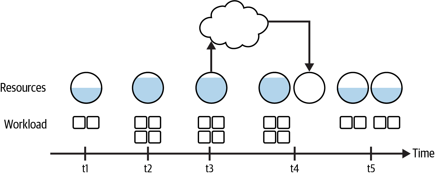
Figure 2-9. Request and rebalance timeline for a scale-out event

Starting at t1, a baseline workload uses about 50% of the compute capacity available. By point t2, the workload has doubled, increasing the load. This increase exceeds a scaling metric, and at t3 the system observes the metric and makes a request for more resources.

Recall from Chapter 1 that it can take some time for additional compute resources to be provided after a capacity request is made. The additional capacity comes online at t4, and the workload rebalances across the additional compute capacity at t5, concluding the scaling event. With the additional capacity to handle the larger workload, the resource utilization returns to the pre-scaling event levels.

You can see an example of this process in how Google Cloud Compute (GCS) uses autoscaling to service high request rates, as detailed in the request rate and access distribution guidelines. This documentation notes that it can be on the order of minutes for GCS to identify high request rates and increase resources. In the interim, responses can slow considerably or fail, because the high request rate exceeds the available capacity. To avoid this issue, users are advised to gradually increase the request rate, which will give GCS time to autoscale.

This is a really important point: failures can occur if request volumes increase before GCS can scale out. You will hit these same types of performance and reliability issues with data processing jobs if you don’t scale out aggressively enough to meet demand for large workloads.

The order of operations is somewhat reversed when you scale in, as illustrated in Figure 2-10. This scenario starts out where things left off in Figure 2-9, with two units of compute capacity running two workload units each. The workload decreases by t2, which results in resource utilization falling for one of the compute units. This triggers a scale-in metric by t3, sending a request to terminate the underutilized compute capacity.

Figure 2-10. Rebalance and removal timeline for a scale-in event

Timepoint t4 in Figure 2-10 is interesting, since a few different things can happen, as depicted by the dashed lines for the workload in t4. In some cases, you can wait for active processes on a node marked for termination to complete. YARN graceful decommissioning is an example of this, where jobs are allowed to complete before a node is decommissioned. This is a good choice for jobs that have a defined end.

The other possibility at t4 is that the compute unit is removed without waiting for processes to finish. In this case, the work being done by that process will have to be retried. This can be the case when scaling in streaming pipelines, where checkpointing can be used to retry jobs killed as a result of decommissioning. In streaming pipelines, you wouldn’t want to use graceful decommissioning as part of your scale-in strategy, as this would block scale-in events.

Ultimately, one compute unit remains after the scale-in event, which picks up the workload from the removed compute unit if necessary.

Warning

While this chapter focuses on autoscaling, there are times when you may manually scale a workload. Ideally these should be exceptional cases, such as experiments or unexpected resource shortfalls—for example, if your cluster has scaled up to the maximum number of workers but more resources are needed, necessitating manual intervention.

If these scenarios start occurring frequently, it’s a sign that either you need to modify your scale-out limits or there are underlying performance issues. Don’t simply throw more resources at a problem. Be sure to monitor and investigate performance degradation.

Common Autoscaling Pitfalls

Scaling plans based on resource utilization and workload state can provide a lot of opportunities to cost-effectively run a pipeline. Time-based autoscaling is great if you have that kind of predictability in pipeline operation, but that isn’t always the case.

Dynamic scaling metrics, such as average memory and CPU utilization, present a challenge as they fluctuate throughout job execution, opening the window for more scaling events to get triggered. This can require a careful balance in how you set up autoscaling plans.

Consider the memory profile for the hypothetical pipeline job shown in Figure 2-11. In the following subsections, I’ll walk through some possible scaling plans for this job to help you get a sense of common pitfalls and how to avoid them.

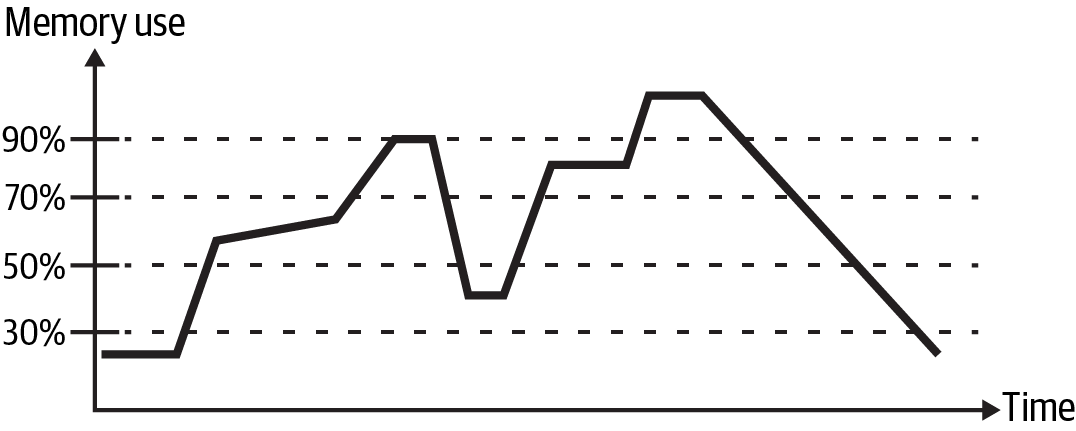
Figure 2-11. Memory profile for a data pipeline job

Scale-out threshold is too high

It’s tempting to think that the scale-out threshold should be high from a cost-effective standpoint; this will prevent prematurely scaling out and wasting compute cycles. While there is some truth to this, you want to balance over-resourcing with sacrificing reliability and performance.

Recall that scaling out is not an instantaneous event; you need to wait for resource provisioning and load rebalancing. Consider the impact of setting the scale-out threshold at 90% for the job depicted in Figure 2-11. In this situation, resources wouldn’t scale out until the memory exceeded this value, potentially impacting reliability.

Keep this in mind when setting scale-out thresholds, and when in doubt, set the scale-out threshold a bit lower than you think you need. You can then monitor resource utilization to see whether this results in a significant number of wasted cycles, and refine thresholds down the road.

Flapping

Not just for birds, flapping or thrashing refers to a cycle of continuously scaling in and out. This can negatively impact performance and reliability, as the load is constantly in a state of rebalancing.

Causes of flapping include:

• Scale-in and scale-out thresholds that are too close together

• An observation window that is too short

You can see flapping with the job depicted in Figure 2-11 if the scale-in threshold is set to 50% and the scale-out threshold is set to 70%. This will result in the three scaling events shown in Figure 2-12, where the lighter shaded bar shows a scale-in event and the darker shaded bars show scale-out events.

Figure 2-12. Flapping due to scale-in and scale-out thresholds that are too close

Figure 2-13 shows the resource allocation resulting from these scaling events. Looking at this view, it’s clear that the scale-in event isn’t necessary, as the resource needs increase immediately following it. In addition to the unnecessary workload shuffling from prematurely scaling in, you can waste compute dollars here. It takes time for resources to spin down, get provisioned, and spin up, all of which you pay for. Another consideration is the granularity of billable time. Some services charge by instance hours and some by fractional hours. Flapping can result in paying this minimum charge multiple times.

One way to resolve the flapping in this example is to increase the observation window for the scale-in event. Notice that the time period that is less than 50% during the shaded interval is much smaller than the time periods that are greater than 70%. If the observation window for the scale-in event was expanded, the 50% time period in Figure 2-12 wouldn’t trigger a scale-in event, leaving resources as is.

Figure 2-13. Resource fluctuation due to flapping

Another solution is to adjust scale-in and scale-out thresholds to be farther apart. If the scale-in threshold was reduced to 30%, the flapping in Figure 2-12 would not occur.

Tip

A rule of thumb for scaling is to scale in conservatively and scale out aggressively. This rule comprehends the overhead of scale-in decommissioning and rebalancing, while giving a nod to the performance and reliability needs for larger workloads.

You can achieve this by setting longer observation windows for scale-in events, and scaling in by a smaller amount than you would scale out by.

Over-scaling

When a scaling event is initiated, it’s critical that you allow enough time for the load to rebalance and the scaling metrics to update. If you don’t, you can end up triggering multiple scaling events that will result in over- or under-resourcing. Over-resourcing wastes money and under-resourcing impacts reliability. This is where the cooldown period comes into play.

Figure 2-14 shows a well-designed autoscaling approach with adequate cooldown. If memory use exceeds 70% for the observation window, a scale-out event is initiated that increases the number of resources by N.

Starting with Poll 1, the memory use remains above 70% for the observation window, triggering a scale-out event. The cooldown period is long enough to account for the scale-out event and resource rebalancing. As a result, the next polling event, Poll 2, occurs after the impact of the N additional resources is reflected in the memory use metric. No additional scaling events are triggered, since the memory use is not above 70%.

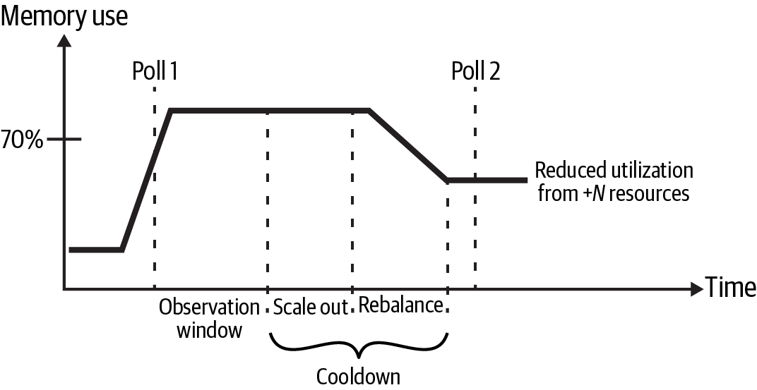
Figure 2-14. Autoscaling example with a sufficient cooldown period

Contrast this with a cooldown period that is too short, as depicted in Figure 2-15. In this case, Poll 2 happens before the impact of the initial scale-out event is reflected in the memory use metric. As a result, a second scale-out event is initiated, resulting in increasing the resources a second time.

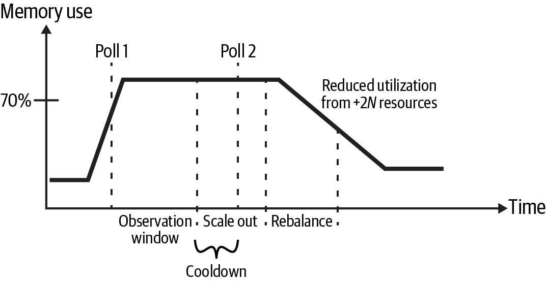
Figure 2-15. Autoscaling example with an insufficient cooldown period

There are two undesirable results here. For one thing, twice as many resources are allocated than needed, which wastes cycles. There’s also the possibility of tipping over into flapping if both the scale-in and scale-out cooldown times are inadequate.

An additional concern when scaling in is under-resourcing resulting from scaling in more than warranted. This is another reason to follow the advice to scale in conservatively and scale out aggressively.

Autoscaling Example

In this section, I’ll walk through an autoscaling plan I developed to show you how benchmarking, monitoring, and autoscaling rules come together to save costs. You’ll also see some of the issues stemming from scaling HDFS and how suboptimal autoscaling can lead to performance and reliability issues.

The pipeline in question ran batch jobs on an on-demand basis in AWS EMR, reading data from cloud storage, copying it to HDFS, and running a Spark job to transform the data. The transformed data was written to cloud storage, where it was accessed by analytics users via a cloud data warehouse. The pipeline operation was variable, as was the workload; some jobs had very little data while others processed significantly more data. This meant scaling was possible due to variation in both pipeline operation and data workload.

Figure 2-16 shows memory and HDFS utilization over the course of the job, with HDFS use shown by the dashed line. You can see how HDFS utilization climbs during the copy step, as data is moved from the cloud onto the cluster. When the copy step finishes and data transformation begins, the memory use ramps up as data is read from HDFS into memory for the Spark transformation. As transformation finishes, memory use ramps down. Following the metastore update, the cluster terminates.

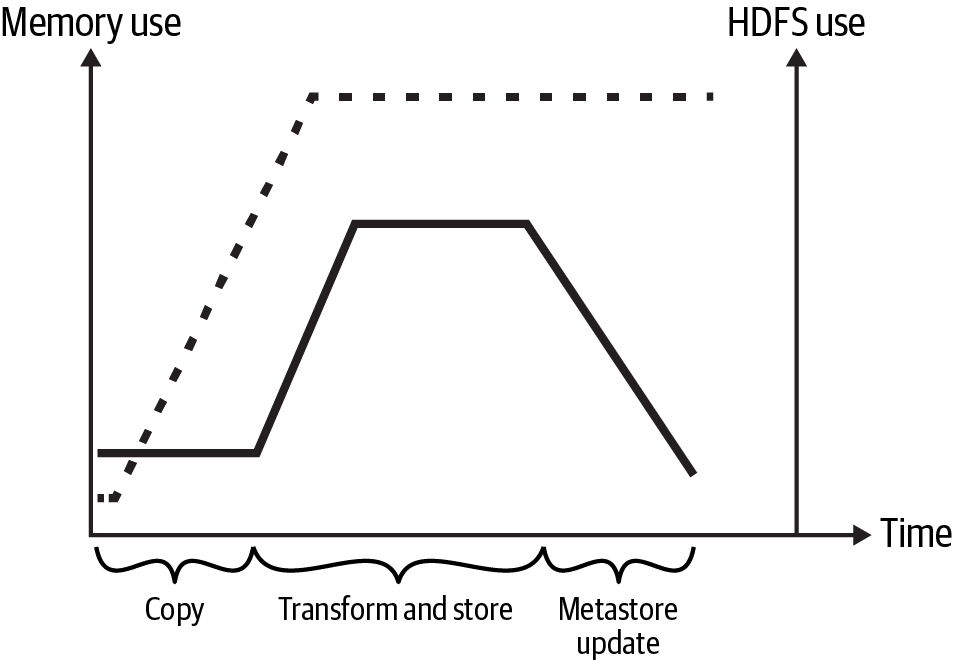
Figure 2-16. Memory and HDFS use over the course of a data ingestion job. HDFS use is depicted by the dashed line.

The pipeline experienced intermittent job failures that traced back to BlockMissin⁠g​Exception. This issue occurs when a block of data is requested but cannot be retrieved from any of the replicas. This exception has several potential causes, but overall it indicates that HDFS is unhealthy. As data size increased, these failures became more frequent, and I took on the task of mitigating the issue.

The original cluster configuration specified an initial number of core nodes⁵ and an autoscaling plan to add or subtract core nodes based on HDFS utilization. Recall from “Designing for Scaling” that scaling HDFS capacity, especially scaling in, is an expensive operation.

You can see how it would be tempting to use HDFS utilization as a scaling parameter in this scenario. The architectural decision to copy data to HDFS and the unknown data load from batch to batch meant that it wasn’t clear how much disk space would be needed until the job started running. By scaling out core nodes based on HDFS utilization, you could simply add more disk space if needed.

Known difficulties with scaling out on HDFS were only part of the issue. The source data exhibited the small-files problem, which you saw in Chapter 1. The additional overhead of having to replicate and keep track of numerous small files exacerbated the difficulties in scaling HDFS.

Another issue was that the mechanism used to copy the data didn’t scale horizontally. If memory use spiked during copy, scaling out for more memory didn’t provide any relief. One final confounding variable was the insufficient resource problem mentioned in Chapter 1: if a scale-out event occurred but no resources were available, the job would stall and ultimately fail.

Altogether, the data characteristics and autoscaling plan resulted in stalled jobs for large datasets. Essentially, as a large set of data was being copied, the HDFS-based autoscaling rules would attempt to scale out. The scale-out events took hours to complete, given the number of small files. The cooldown period was set to five minutes, so multiple scaling events would trigger during this time, like the issue depicted in Figure 2-15. As a result of the constant reconfiguration of HDFS space, eventually a block would not be found, causing the job to fail.

The job failures were certainly a negative, but the cloud bill costs were another issue. Hours-long autoscaling events drove up job runtime, which drove up costs and made the system unstable.

Reducing failures involved improving the autoscaling rules and modifying the architecture to ensure that jobs had sufficient resources to succeed at the copy step.

On the architecture side, task nodes were added to the cluster configuration. The scaling strategy was modified to scale only the number of task nodes; the number of core nodes remained fixed. Rather than scale on HDFS utilization, the task nodes were scaled based on YARN memory and container metrics. You can see all of these metrics in the EMR autoscaling metrics documentation.

This eliminated the issues of scaling based on HDFS, but it didn’t address the fact that the amount of disk space needed varied from job to job. This is where benchmarking came in.

I plotted the various data sizes and cluster configurations for successful ingestion jobs. This gave me a starting point for identifying the number of core nodes required for a successful job. I separated jobs into high, medium, and low data size based on these metrics, and I added a step in the cluster launch process that checked the size of the incoming data. The initial cluster configuration would use the number of core nodes based on the data size falling into the high, medium, or low bucket and the min and max limits for scaling the workers. In this way, cost was optimized based on data workload, and the single-threaded copy stage would succeed because the core node count was fixed at the required capacity.

Because this process surfaced the data size, I could also set the EBS volume size to ensure that there would be enough capacity to run the job, eliminating the need to scale out disk space. I came up with a conservative approximation based on data size, replication factor, and disk space needed for data transformation.

With these changes, autoscaling events occurred only during data transformation as more resources were needed to process the data. This approach eliminated the long-running autoscaling events and significantly reduced the job failure rate. In addition, the workload-based cluster and autoscale configurations improved reliability by guaranteeing sufficient HDFS capacity from the outset.

Summary

Variety is the spice of life, and variation is the sign that a pipeline can take advantage of scaling, leveraging cloud elasticity to minimize costs by scaling in and to keep up with increased demand by scaling out.

Answering the following questions will help you uncover sources of variability and their predictors in data pipelines:

• How does pipeline operation change over time?

• How does data workload vary?

• How does variation in data workload or operation impact resource needs?

• How do you know that resource needs are changing?

Pipelines with variable operation provide opportunities to reduce costs when there are fewer active jobs. Variation in data workload can be leveraged to reduce costs for smaller workloads without sacrificing performance for larger workloads.

There are multiple levels at which you can scale. At the system level, pipelines with periodic operation can take advantage of scheduled autoscaling, reducing costs during known quiescent times. When operation variability is less predictable, resource use and system metrics can be used to trigger scaling events.

At the level of data processing, workload variation can provide opportunities to scale in for less complex workloads while scaling out to support higher volumes and complexity. You can also scale within data processing jobs, such as with Spark dynamic resource allocation, to take advantage of differing resource needs across data processing stages.

Determining when to scale involves identifying meaningful metrics that indicate whether more or fewer resources are needed. Benchmarking different workloads can help you identify a starting point for these metrics, as well as appropriate thresholds and observation windows for making scaling decisions.

Designing pipelines to take advantage of distributed data processing is essential for horizontal scaling. Careful code design, partitioning, and being aware of shuffle will help you get the most out of this strategy.

When scaling out data processing, account for the impacts of increased data volume and size on services the pipeline interacts with. Take care to ensure that consumers can manage increased workloads, and be cognizant of impacts to quotas and throttling limits.

Favoring cloud storage will improve pipeline scalability and can reduce costs. Scaling HDFS is not recommended due to long decommissioning times; furthermore, databases couple storage and compute, necessitating scale-up of both. Separating storage and compute gives you the faster bandwidth of cloud storage and eliminates the compute cost associated with databases.

Automatically adjusting resource allocation is a delicate balancing act. When developing scaling plans, leave adequate time for the following:

• Scaling events to conclude, such that resources have been added or removed

• Workloads to rebalance across the changed resource envelope

• Metrics to update, ensuring that the next scaling decision is made based on the impacts of the previous scaling event

Scaling out aggressively helps you keep up with rapidly increasing workloads, while scaling in conservatively minimizes decommissioning overhead, under-resourcing, and double costs for terminating compute just to request it again.

Common issues stem from setting thresholds too high or too close together and from not having adequate cooldown and observation window durations. The following recommendations will help you avoid degraded performance and reliability when scaling:

• Set scale-out thresholds low enough to allow time for new resources to come online and load rebalancing to occur before critical performance or reliability limits are hit.

• Provide enough time between scaling events (i.e., cooldown) to give resources time to rebalance.

• Set scale-in and scale-out thresholds sufficiently far apart to avoid flapping.

• Ensure that your observation window is wide enough to avoid premature scaling events. Scaling too early can cause flapping, and scaling too late can miss cost optimization opportunities.

This and the preceding chapter focused on navigating the cost–performance trade-offs of cloud compute, with strategies for resource sizing, pricing, and scaling specifically for data pipeline workloads. The themes of size, cost, and scaling continue in the next chapter on cloud storage, where you’ll see how to minimize storage costs and structure files for efficient data processing.

Recommended Readings

• The “Autoscaling” article in the Azure Architecture documentation, which does a particularly good job of describing autoscaling best practices

• The “Design for scaling” article from the Microsoft Azure Well-Architected Framework

• Scaling in Kubernetes

  • “Horizontal Pod Autoscaling”

  • Issue about scaling to zero

• Spark adaptive query execution explainer from Databricks

• DoorDash’s “Building Scalable Real Time Event Processing with Kafka and Flink”

• High Performance Spark by Holden Karau and Rachel Warren (O’Reilly)